Active Flutter Suppression of a Wing Section in a Compressible Flow

Abstract

In this paper, a unified method for the computation of the unsteady aerodynamic forces in the Laplace domain for a wing section in subsonic, sonic and supersonic potential flows is presented. The subsonic solution is a new development based on the pressure mode method. The unsteady aerodynamic forces are evaluated in the Laplace domain by an efficient method for computing the kernel. The sonic potential flow solution is an extension of the solution for the frequency domain to the Laplace domain. Analytical expressions for the unsteady pressure coefficient and the unsteady aerodynamic forces in the Laplace domain are obtained for this flow regime. The method is validated in these regimes with existing theories in the frequency domain, and its application to flutter computation is provided for different Mach numbers by the use of the p-method. Active flutter suppression for a wing section with three degrees of freedom has been studied, and an adequate control law has been obtained. Using the proposed approach allows to calculate the unsteady aerodynamic forces directly in the Laplace domain, avoiding the inconvenience of the curve fitting from the frequency to the Laplace domain. In particular, this work can be used as a base for the application of other procedures for flutter suppression in the transonic regime.

1. Introduction

With the objective of fuel consumption reduction, new high-aspect-ratio wings are being developed. This will certainly lead to less stable aircraft configurations, with an increasing tendency to flutter occurrence [1]. A solution to such aeroelastic instabilities is reached by the use of active flutter suppression systems (AFS) [2]. The first demonstration of an active flutter suppression system was carried out by the USAF in 1973 [3]. A B-52 bomber was converted to a Control Configured Vehicle (CCV), with its stability intentionally deteriorated so that flutter would occur within its flight envelope [4]. Once the new flutter velocity was determined, the CCV was equipped with a flutter suppression system, with flight experiments showing an increase of at least 10 knots of flutter speed, setting a precedent for future research. Livne [4] presents an overview of over fifty years of research and development in AFS.

AFS can provide then a powerful and effective solution to flutter problems. When included in the aircraft design procedure from its beginning, AFS can lead to weight saving and more efficient airframes [4]. However, in order to guarantee a safe application, aeroelastic and aeroservoelastic analysis and simulation improvements are certainly needed. Benchmark Active Control Technology (BACT) has been extensively investigated for flutter suppression by several authors (see for example [5,6]) for studying transonic aeroelastic phenomena. In the work of Waszak [5], wind tunnel data of unsteady aerodynamics near transonic flutter conditions were required for the design and implementation of AFS.

Special attention must be paid to the calculations in the transonic regime, where unsteady aerodynamic forces must be obtained, either by wind tunnel measurements or by numerical computer methods, to properly account for nonlinearities. Baker [7] presents a correction of linear aerodynamics that avoids high computational costs when a large number of flight conditions need to be evaluated, providing that steady or unsteady wind tunnel data are available. In addition, Vepa and Kwon [8] present a method for AFS in the transonic domain introducing control laws, derived from linear unsteady aerodynamics and implemented using a nonlinear transonic small disturbance method for AFS. This seems to be a highly promising approach, since nonlinear aerodynamic computations are avoided, although a reliable linear method in the compressible domain is required.

Traditional flutter calculation methods use the assumption of simple harmonic oscillations. With the advent of active control technology for flutter suppression and gust load alleviation, and in order to predict correct sub- and supercritical flutter behavior, the use of Laplace or time domains becomes essential. The main difficulty of these formulations lies in obtaining the unsteady aerodynamic forces for arbitrary wing motions. Rational function approximations (RFA) (see for example Vepa [9] and Rogers [10]) approximate the unsteady aerodynamic forces in complex p-plane, based on those obtained for simple harmonic oscillations (forces computed on the imaginary axis only). With the use of RFA, certain error is introduced into the resulting aeroservoelastic model due to inaccuracies in the RFA/frequency domain data fit. More important, additional states are generated, which are unmeasurable and very sensitive to the modeling adopted [11]. Thus, the use of this procedure to obtain robust control laws may be inaccurate.

The works of Edwards [12], Ueda [13] and Quero [14] have contributed to the calculation of Laplace domain aerodynamics in the 2D and 3D area, respectively. The former used the classical theories of Theodorsen and of Garrick and Rubinov [15], and they obtained the corresponding p-domain solutions for incompressible and supersonic flows. Ueda has further generalized his doublet point method [13] to the p-domain for 3D subsonic lifting surfaces.

In the time domain, the use of indicial aerodynamics function, see for example the works of Leishman [16] and Djayapartapa et al. [17] for two-dimensional compressible flow, is another option for AFS, although it requires a large amount of computational resources.

It is our objective to formulate a direct method to calculate the Laplace transformed pressure distribution on lifting airfoils for any compressible regime. For the subsonic case in potential flow, Possio´s [18] integral equation is generalized to the p-domain, and the resulting kernel is recast to display its singularities explicitly. Then, the kernel is integrated numerically, except for the singular term, which is integrated analytically. Second, the pressure mode method is applied, and the integral equation is evaluated at a set of discrete points. For the sonic case, the solution of Rott [19] is generalized to the Laplace plane. For supersonic flows, the work of Edwards [12] is implemented. In the transonic regime, a curve fit is used on the unsteady generalized forces in the Laplace domain based on the results obtained by the three aforementioned theories. Finally, with the use of these unsteady loads, this study aims to calculate the flutter velocity of a wing section and to develop a closed-loop control law to increase its stability and expand its flight envelope for any compressible regime.

2. Equations of Motion

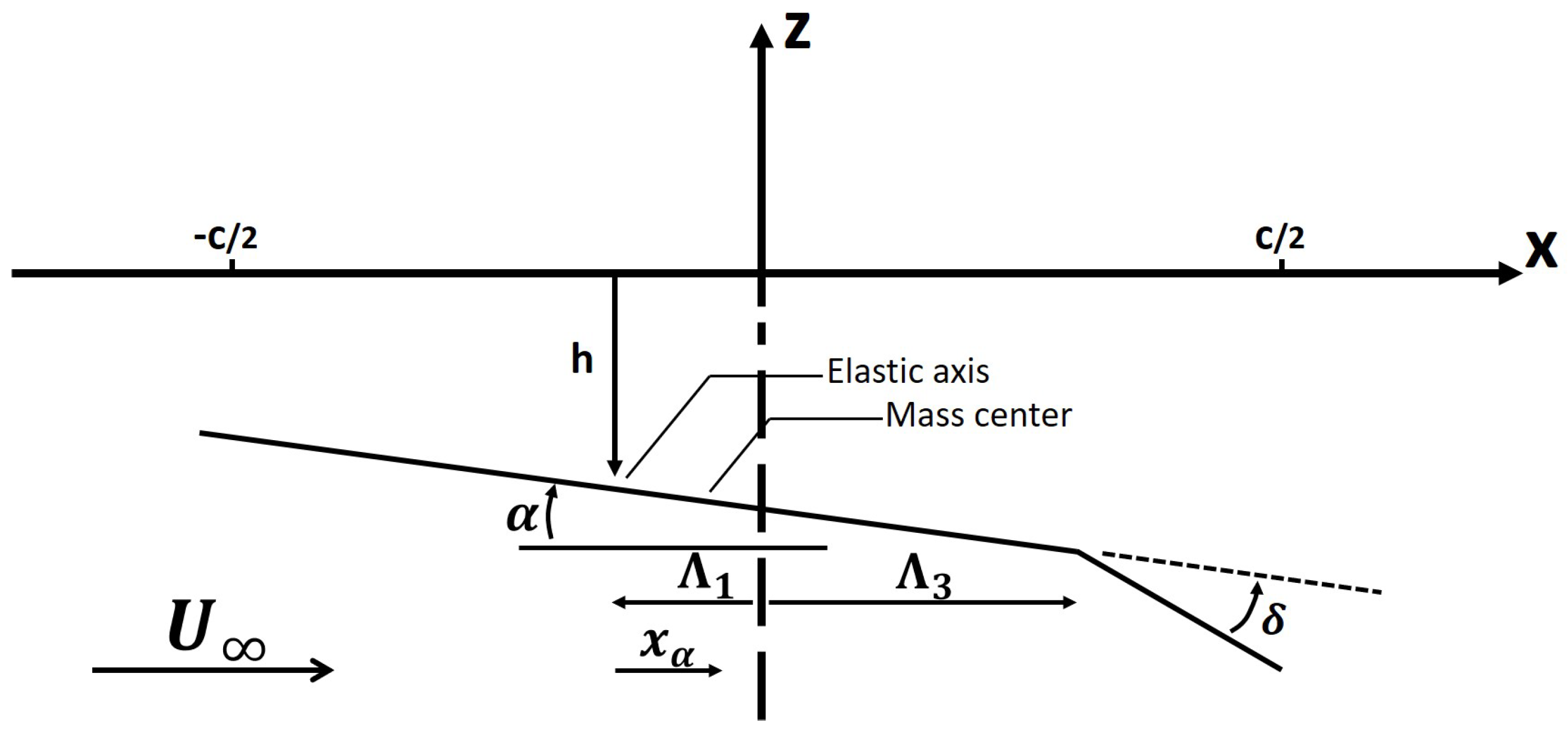
The aeroelastic characteristics of a high aspect ratio wing can be determined in first approximation by considering the two-dimensional section located at 70% of the wing root (see [20]). The three degrees of freedom system is presented in Figure 1. The resulting equations that describe the dynamic motion of the system are nondimensionalized with the section mass $m_s$ and the semichord $c/2$:

$$\begin{array}{c}\hfill \left[\begin{array}{ccc}1& x_{\alpha }& x_{\delta }\\ x_{\alpha }& r_{\alpha }^2& r_{\delta }^2+{\Lambda }_{31}{x}_{\delta }\\ x_{\delta }& r_{\delta }^2+{\Lambda }_{31}{x}_{\delta }& r_{\delta }^2\end{array}\right]\left\{\begin{array}{c}\ddot{q}\end{array}\right\}+\left[\begin{array}{ccc}0& 0& 0\\ 0& 0& 0\\ 0& 0& 2r_{\delta }^2{\omega }_{\delta }{\zeta }_{\delta }\end{array}\right]\left\{\begin{array}{c}\dot{q}\end{array}\right\}+\\ \hfill +\left[\begin{array}{ccc}{\omega }_h^2& 0& 0\\ 0& r_{\delta }^2{\omega }_{\alpha }^2& 0\\ 0& 0& r_{\delta }^2{\omega }_{\delta }^2\end{array}\right]\left\{\begin{array}{c}q\end{array}\right\}=\frac{1}{m_s{(c/2)}^2}\left\{\begin{array}{c}{Q}_h\frac{c}{2}\\ Q_{\alpha }\\ Q_{\delta }\end{array}\right\}\end{array}$$

(1)

where $x_{\alpha }$ is the nondimensional distance from the center of mass to the elastic axis, $r_{\alpha }^2$ is the nondimensional radius of gyration of the airfoil, $x_{\delta }$ is the nondimensional distance from the center of mass of the control surface to the hinge axis, $r_{\delta }^2$ is the nondimensional radius of gyration of the control surface, ${\Lambda }_{31}$ is the nondimensional distance between the elastic axis and the hinge axis of the control surface, ${\zeta }_{\delta }$ is the nondimensional damping coefficient of the control surface mode and $\left\{q\right\}={\left[\frac{h}{\frac{c}{2}}\alpha \delta \right]}^T$.

For linear aerodynamics, the right-hand side of Equation (1) can be expressed as:

$$\frac{1}{m_s{(c/2)}^2}\left[\begin{array}{c}{Q}_h\frac{c}{2}\\ Q_{\alpha }\\ Q_{\delta }\end{array}\right]=\frac{{\rho }_{\infty }{U}_{\infty }^2}{2m_s}\left[Q_{ij}\right]\left\{\begin{array}{c}q\end{array}\right\}$$

(2)

For aeroservoelastic applications, Equation (1) can be solved either in the time domain or in the Laplace domain.

However, the solution in the Laplace domain involves the computation of the generalized unsteady aerodynamic forces (matrix $\left[Q_{ij}\right]$) in the Laplace domain. This can be completed either directly in this domain, or it can rather be determined by a curve-fitting method such as the one proposed by Vepa [9] among others, extrapolating the results from the frequency domain to the Laplace domain. In this work, a unified method to determine the aerodynamic generalized force matrix $\left[Q_{ij}\right]$ in the Laplace domain for a compressible flow will be implemented, avoiding thus the inaccuracies of the curve-fitting process.

3. Unsteady Aerodynamic Forces

Small disturbance unsteady aerodynamic potential will be assumed for the cases of subsonic, sonic and supersonic flows. Linear potential theory has been used classically for incompressible, subsonic and supersonic flows, see for example [15,21]. However, in the transonic regime, it is well known that the linear potential theory is unable to describe accurately the main characteristics of the flow. Despite this, sonic linear theory [22] provides a limiting value and avoids the singularity of linear subsonic or supersonic solutions when the Mach number approaches one. Unsteady sonic solutions have been used in the frequency domain by [19] among others. In this work, the same arguments used by these authors will be taken into account, with this limiting value applied to the Laplace domain. As it will be shown in the results presented hereafter, linear sonic theory is able to provide an accurate finite value for the flutter characteristics of the wing section, being thus a starting point for the nonlinear transonic flutter computations, which are more complex and require higher computational resources.

In what follows, all lengths are nondimensionalized with the airfoil semichord $c/2$, velocities with the freestream velocity $U_{\infty }$ and pressures with the freestream dynamic pressure.

3.1. Unsteady Subsonic Flow

In order to study stability phenomena, the initial conditions of the problem can be ignored. The integral equation relating the downwash velocity to the pressure coefficient on the airfoil in the Laplace domain can be expressed after Possio [18] by replacing the nondimensional frequency variable k by the nondimensional Laplace variable s as

$$w\left(x,0;s\right)=\frac{\beta }{4\pi }{\int }_{-1}^{1}K(x-\xi ,M_{\infty };s)·\Delta C_P\left(\xi \right)d\xi$$

(3)

where $s=\frac{pc}{2U_{\infty }}$ (p being the dimensional Laplace transform variable), x is the chordwise spatial coordinate (nondimensional unless otherwise stated) and K is the kernel of the integral equation.

Following [23], the kernel is recast as one regular and two singular terms in the form

$$K\left(x-\xi ,M_{\infty };s\right)=\frac{1}{x-\xi }+K_1(x-\xi ,M_{\infty };s)log|x-\xi |+K_2(x-\xi ,M_{\infty };s)$$

(4)

where

$$\begin{array}{cc}\hfill K_1(x-\xi ,M_{\infty };s)& =-\frac{s}{{\beta }^2}{e}^{-s(x-\xi )}{F}_1(x-\xi ,M_{\infty };s)\hfill \\ \hfill K_2(x-\xi ,M_{\infty };s)& =-e^{-s(x-\xi )}{F}_2(x-\xi ,M_{\infty };s)\hfill \\ \hfill & \\ \hfill F_1(x-\xi ,M_{\infty };s)& =\left[J_0\left(z\right)-i{M}_{\infty }{J}_1\left(z\right)\right]e^{\frac{s(x-\xi )}{{\beta }^2}}-s(x-\xi ){\int }_0^1{e}^{zu}{J}_0\left(zu\right)du\hfill \\ \hfill F_2(x-\xi ,M_{\infty };s)& =[\frac{e^{-\frac{s{M}_{\infty }^2(x-\xi )}{{\beta }^2}}-1}{(x-\xi )}+\frac{is}{2{\beta }^2}{J}_0\left(z\right)+\frac{s}{{\beta }^2}{G}_0\left(z\right)+\frac{s}{{\beta }^2}\left(\gamma +log\frac{M_{\infty }s}{2i{\beta }^2}\right)J_0\left(z\right)+\hfill \\ \hfill & +\frac{s\pi M_{\infty }}{2{\beta }^2}{J}_1\left(z\right)-\frac{is{M}_{\infty }}{{\beta }^2}log\frac{M_{\infty }s}{2i\beta }{J}_1\left(z\right)+\frac{is{M}_{\infty }}{{\beta }^2}{G}_1\left(z\right)]e^{\frac{s(x-\xi )}{{\beta }^2}}+\hfill \\ & +\frac{s}{\beta }log\frac{1+\beta }{M_{\infty }}-\frac{i\pi s^2(x-\xi )}{2{\beta }^2}{\int }_0^1{e}^{zu}\left[J_0\left(zu\right)-\frac{2i}{\pi }{G}_0\left(zu\right)\right]du+\hfill \\ \hfill & -\frac{s^2(x-\xi )}{{\beta }^2}\left(\gamma +log\frac{M_{\infty }s}{2i{\beta }^2}\right){\int }_0^1{e}^{zu}{J}_0\left(zu\right)du+\frac{s^2(x-\xi )}{{\beta }^2}{\int }_0^{1}log\frac{1}{u}{e}^{zu}{J}_0\left(zu\right)du\hfill \end{array}$$

(5)

$J_0$ and $J_1$ are Bessel functions of the first kind of order 0 and 1, respectively, $z=\frac{M_{\infty }s\left|x-\xi \right|}{i{\beta }^2}$, $M_{\infty }$ the freestream Mach number, ${\beta }^2=1-M_{\infty }^2$ and the functions $G_0$ and $G_1$, are

$$\begin{array}{cc}\hfill G_0\left(z\right)& =+\frac{\pi }{2}{Y}_0\left(z\right)-\left(\gamma +log\frac{z}{2}\right)J_0\left(z\right)\hfill \\ \hfill G_1\left(z\right)& =-\frac{\pi }{2}{Y}_1\left(z\right)-\frac{1}{z}+log\frac{z}{2}{J}_1\left(z\right)\hfill \end{array}$$

(6)

where $Y_0$ and $Y_1$ are Bessel functions of the second kind of order 0 and 1.

It is important to note that the functions $F_1$ and $F_2$ are all analytic and that when $M_{\infty }$ approaches zero, they are properly reduced to their incompressible counterpart.

Solution of the Integral Equation

A pressure mode method is adopted to solve the integral equation. The pressure coefficient over the airfoil is assumed to be of the form

$$\Delta C_P\left(\xi \right)=\sqrt{\frac{1-\xi }{1+\xi }}\sum _{n=0}^N{a}_n·u_n\left(\xi \right)$$

(7)

where

$$u_n\left(\xi \right)=\frac{sin\left[\left(n+\frac{1}{2}\right){cos}^{-1}\xi \right]}{sin\left[\frac{1}{2}{cos}^{-1}\xi \right]}$$

(8)

and the $a_n$ are $N+1$ constants that are determined by evaluation of the integral equation at $N+1$ collocation points. The advantage of this expression for the pressure distribution lies in the fact that it properly models the singularity at the leading edge and the known square root behavior at the trailing edge.

Bland [23] has shown that the error in the curve fitting of the downwash w is minimized if the collocation points where the integral equation is evaluated are taken as

$$x_j=cos\frac{2i\pi }{2N+1}i=1,...,N+1$$

(9)

We thus obtain a system of $N+1$ equations of the form

$$w\left(x_i,0;s\right)=\frac{\beta }{4\pi }\sum _{n=0}^N{a}_n{\int }_{-1}^1\sqrt{\frac{1-\xi }{1+\xi }}{u}_n\left(\xi \right)K(x_i-\xi ,M_{\infty };s)d\xi i=1,...,N+1$$

(10)

the downwash velocity at $x_i$ is obtained from tangency boundary condition on the airfoil

$$w\left(x_i,0;s\right)=(s+\frac{\partial }{\partial x})\overline{z}(x_i,s)$$

(11)

where $\overline{z}(x_i,s)$ is the Laplace transformed airfoil deflection.

The integral of the right-hand side is divided into three parts. The first one is given by

$${\int }_{-1}^1\sqrt{\frac{1-\xi }{1+\xi }}{u}_n\left(\xi \right)\frac{1}{x_i-\xi }d\xi$$

(12)

This integral, that contains the term with the strongest singularity, can be obtained however analytically because of the simplicity of the function.

To evaluate the second one,

$${\int }_{-1}^1\sqrt{\frac{1-\xi }{1+\xi }}{u}_n\left(\xi \right)K_1\left(x_i-\xi ,M_{\infty };s\right)log\left|x_i-\xi \right|d\xi$$

(13)

the interval is divided into four subintervals [24], and each of the arising integrals is obtained numerically by a Gaussian quadrature.

Finally, the third integral

$${\int }_{-1}^1\sqrt{\frac{1-\xi }{1+\xi }}{u}_n\left(\xi \right)K_2\left(x_i-\xi ,M_{\infty };s\right)d\xi$$

(14)

is approximated by a $N+1$ point Jacobi–Gaussian quadrature

$${\int }_{-1}^1\sqrt{\frac{1-\xi }{1+\xi }}{u}_n\left(\xi \right)K_2\left(x_i-\xi ,M_{\infty };s\right)d\xi \equiv \pi \sum _{j=1}^{N+1}{u}_n\left({\xi }_j\right)K_2\left(x_i-{\xi }_j,M_{\infty };s\right)$$

(15)

where ${\xi }_j$ are the zeros of the airfoil polynomial $u_{N+1}\left(\xi \right)$.

Thus, we arrive to a system of $N+1$ equations of the form

$$\left\{w\left(x_i\right)\right\}=\left[c_{ij}\right]\left\{a_j\right\}$$

(16)

where $c_{ij}$ are the sum of the coefficients of $a_j$ in the above integrals at the collocation points $x_i$.

The convergence of the method was extensively studied by Fromme and Golgberg [24]. For most of the computations presented, ten to twelve terms were enough to guarantee a converged solution, even when the airfoil had a kink as in the case of the oscillating control surface.

The generalized forces can be obtained by analytical integration of the pressure coefficient and shown to be functions of the $a_n$ only. Thus, once we obtain the constants $a_n$, we can evaluate the generalized forces just by algebraic operations.

3.2. Unsteady Sonic Flow

The linearized equation for the compressible loads presents a singularity at $M_{\infty }=1$. Therefore, it cannot be used to study flows in the proximity of this Mach number. In order to obtain the solution for this regime, the limit $M_{\infty }\to 1$ must be imposed in the velocity potential equation [19].

The equation for the nondimensional unsteady velocity potential at $M_{\infty }=1$ is

$${\varphi }_{zz}-{\varphi }_{tt}-2{\varphi }_{xt}=0$$

(17)

With the following boundary conditions

$$\begin{array}{cc}\hfill & z\to \infty \hfill \\ \hfill & x>=0\hfill \\ \hfill & x<0\hfill \end{array}\begin{array}{cc}\hfill & \varphi (x,z,t)\to 0\hfill \\ \hfill & \frac{\partial }{\partial z}\varphi (x,z=0^{\pm },t)=w(x,t)\hfill \\ \hfill & \varphi (x,z,t)=0\hfill \end{array}$$

(18)

Applying the Laplace transformation to the velocity potential, two functions are defined:

$$\mathcal{L}\left\{\varphi (x,z,t)\right\}={\int }_0^{\infty }{e}^{-st}\varphi (x,z,t)dt=\varphi (x,z,s)+{\varphi }^{\prime }(x,z,s)$$

(19)

This expression can be manipulated in such a way that ${\varphi }^{\prime }$ fulfills all initial conditions with null boundary conditions, while $\varphi$ does it with null initial conditions.

Since initial conditions do not affect the stability problem, only this last part of the velocity potential will be studied. The governing equation for potential $\varphi$ is then

$${\varphi }_{zz}-s^2\varphi -2s{\varphi }_x=0$$

(20)

Defining the Laplace transformation of the velocity potential with respect to the abscissa x

$$\phi (\lambda ,z,s)={\mathcal{L}}_x\left[\varphi (x,z,s)\right]={\int }_0^{\infty }{e}^{-\lambda x}\varphi (x,z,s)dx$$

(21)

where ${\mathcal{L}}_x$ is the Laplace transform with respect to the variable x.

Equation (20) can be solved, obtaining

$$\begin{array}{cc}\hfill & \phi (\lambda ,z,s)=-\frac{{\mathcal{L}}_x\left[w(x,s)\right]}{\nu }{e}^{-\nu z}\hfill \\ \hfill & \phi (\lambda ,z,s)=+\frac{{\mathcal{L}}_x\left[w(x,s)\right]}{\nu }{e}^{+\nu z}\hfill \end{array}\begin{array}{cc}\hfill & z>0\hfill \\ \hfill & z<0\hfill \end{array}$$

(22)

where $\nu$ is

$${\nu }^2=2s\left(\lambda +\frac{s}{2}\right)$$

(23)

Finally, by applying the inverse Laplace transformation, the velocity potential can be calculated:

$${\mathcal{L}}^{-1}\left(\phi \right)=-{\int }_0^{\infty }\frac{w(\xi ,s)}{\sqrt{2s\pi }}\frac{exp\left[-s\left(x-\xi -\frac{z^2}{\sqrt{x-\xi }}\right)\right]}{\sqrt{x-\xi }}d\xi$$

(24)

and can be particularized on the surface of the airfoil, by taking the limit $z\to 0^{\pm }$.

$$\varphi (x,s)=-{\int }_0^x\frac{w(\xi ,s)}{\sqrt{\pi s(x-\xi )}}{e}^{-s(x-\xi )}d\xi$$

(25)

The pressure coefficient is defined as:

$$Cp=-2\frac{\partial \varphi }{\partial t}-2\frac{\partial \varphi }{\partial x}$$

(26)

Introducing the change of variable $x-\xi =\eta$, the final equation for this pressure coefficient is:

$$Cp=\frac{1}{\sqrt{\pi s}}{\int }_0^x\frac{2sw(x-\eta ,s)+\frac{\partial }{\partial x}\left(w(x-\eta ,s)\right)}{\sqrt{\eta }}{e}^{-s\eta }d\eta +\frac{w(0,s)}{\sqrt{\pi sx}}{e}^{-sx}$$

(27)

Introducing the parameters for a 2D airfoil, with $x_0=\frac{{\Lambda }_1+1}{2}$ and $x_1=\frac{{\Lambda }_3+1}{2}$, an analytical expression for the unsteady pressure coefficient is reached in the form

$$\begin{array}{c}\hfill \begin{array}{cc}\hfill Cp=& [\left(\frac{a_1+a_3}{s}-\frac{b_1+b_3}{2s^2}\right)erf\left(\sqrt{sx}\right)-\left(\frac{a_3}{s}-\frac{b_3}{2s^2}\right)erf\left(\sqrt{s(x-x_1)}\right)\hfill \\ \hfill & +\frac{(b_1+b_3)\sqrt{x}}{s^{3/2}\sqrt{\pi }}{e}^{-sx}-\frac{b_3\sqrt{x-x_1}}{s^{3/2}\sqrt{\pi }}{e}^{-s(x-x_1)}]\left\{\begin{array}{c}\frac{h}{c/2}\\ \alpha \\ \delta \end{array}\right\}+\frac{w(0,s)}{\sqrt{\pi sx}}{e}^{-sx}\hfill \end{array}\end{array}$$

(28)

where

$$\begin{array}{c}\hfill \begin{array}{cc}\hfill a_1& =\left[\begin{array}{ccc}2s^2,& 4s+4s^2(x-x_0),& 0\end{array}\right]\hfill \\ \hfill a_3& =\left[\begin{array}{ccc}0,& 0,& 4s+4s^2(x-x_1)\end{array}\right]\hfill \\ \hfill b_1& =\left[\begin{array}{ccc}0,& 4s^2,& 0\end{array}\right]\hfill \\ \hfill b_3& =\left[\begin{array}{ccc}0,& 0,& 4s^2\end{array}\right]\hfill \end{array}\end{array}$$

(29)

The aerodynamic loads are finally computed by integration of the pressure distribution.

3.3. Unsteady Supersonic Flow

The procedure to compute the unsteady aerodynamic forces in supersonic flow is the one presented by Edwards [12]. A brief summary is given here for completeness.

The equation for the velocity potential is

$$\varphi (x,0^{+},t)=\frac{1}{\sqrt{M_{\infty }^2-1}}{\int }_0^x{w}_a(\xi ,s)exp\left[-\frac{s{M}_{\infty }}{M_{\infty }^2-1}(x-\xi )\right]J_0\left[-i\frac{s{M}_{\infty }}{M_{\infty }^2-1}(x-\xi )\right]d\xi$$

(30)

Garrick and Rubinov [15] obtained the solution for the simple harmonic forces. Following Garrick´s notation and generalizing these loads to the Laplace domain

$$\left\{\begin{array}{c}{Q}_h\frac{c}{2}\\ Q_{\alpha }\\ Q_{\delta }\end{array}\right\}=-\frac{8\rho {\left(\frac{c}{2}\right)}^2{U}_{\infty }^2}{\sqrt{M_{\infty }^2-1}}\left[M_a{s}^2+B_{a}s+K_a\right]\left\{\begin{array}{c}\frac{h}{c/2}\\ \alpha \\ \delta \end{array}\right\}$$

(31)

with the matrices being

$$\begin{array}{c}\hfill \begin{array}{cc}\hfill M_a=& \left[\begin{array}{ccc}{r}_2& (r_3-2x_0{r}_2)& t_3\\ (q_2-2x_0{r}_2)& (\frac{2}{3}{q}_3-2x_0(q_2+r_3)+4x_0^2{r}_2)& (\frac{2}{3}{s}_3+2t_3(x_1-x_0))\\ p_2& (\frac{2}{3}{p}_3-2x_0{p}_2)& \frac{2}{3}{s}_3\end{array}\right]\hfill \\ \hfill B_a=& \left[\begin{array}{ccc}\frac{1}{2}{r}_1& (2r_2-x_0{r}_1)& 2t_2\\ (q_1-x_0{r}_1)& (2q_2-2x_0(q_1+2r_2)+2x_0^2{r}_1)& (2s_2+4t_2(x_1-x_0))\\ p_1& 2(p_2-x_0{p}_1)& 2s_2\end{array}\right]\hfill \\ \hfill K_a=& \left[\begin{array}{ccc}0& \frac{1}{2}{r}_1& \frac{1}{2}{t}_1\\ 0& (q_1-x_0{r}_1)& (s_1+t_1(x_1-x_0))\\ 0& p_1& s_1\end{array}\right]\hfill \end{array}\end{array}$$

(32)

parameters $q_i$, $r_i$, $s_i$ and $t_i$ are functions of s derived from the Schwartz function and can be found in [25].

3.4. Unsteady Transonic Flow

It is well known that transonic regime is extremely nonlinear, since it is dominated by moving shock waves. In addition, neither the subsonic nor the supersonic theories previously presented are applicable in the transonic regime, since a singularity appears at $M_{\infty }=1$. A nonlinear theory should be followed to obtain a valid method to study transonic phenomena. However, this approach demands high computing times, hence the need for a solution as a first approach compatible with the classical linear solutions used for subsonic and supersonic flows. Therefore, as a first approximation, the transonic unsteady aerodynamic forces will be obtained by interpolation from the known values of subsonic, sonic and supersonic forces.

In the first place, an expression for the interpolation of the transonic loads must be chosen. The values of the aerodynamic coefficients must be continuous and differentiable over the Mach number, and therefore, the following conditions are imposed

$$\begin{array}{cc}\hfill Q_{transonic}(M_{\infty }=0.85)& =Q_{subsonic}(M_{\infty }=0.85)\hfill \\ \hfill {\dot{Q}}_{transonic}(M_{\infty }=0.85)& ={\dot{Q}}_{subsonic}(M_{\infty }=0.85)\hfill \\ \hfill Q_{transonic}(M_{\infty }=1.00)& =Q_{sonic}\hfill \\ \hfill Q_{transonic}(M_{\infty }=1.15)& =Q_{supersonic}(M_{\infty }=1.15)\hfill \\ \hfill {\dot{Q}}_{transonic}(M_{\infty }=1.15)& ={\dot{Q}}_{supersonic}(M_{\infty }=1.15)\hfill \end{array}$$

(33)

In order to fulfill these conditions, the use of two third-order polynomials, one for the subsonic region and one for the supersonic region, are used with a new condition imposed to calculate the polynomial coefficients:

$${\dot{Q}}_{transonic}(M_{\infty }=1^{-})={\dot{Q}}_{transonic}(M_{\infty }=1^{+})=\frac{Q_{supersonic}(M_{\infty }=1.15)-Q_{subsonic}(M_{\infty }=0.85)}{1.15-0.85}$$

(34)

With this condition, the slope at sonic speed is bounded, minimizing the influence of one region on another. Unwanted relative extrema are minimized while maintaining a continuous and smooth interpolation.

4. Stability of Open-Loop Dynamic System

Once the unsteady aerodynamic forces have been computed in the Laplace domain, it is possible to analyze the stability of the system in this plane. First, the stability matrix of the system in open loop is obtained

$$\left|\begin{array}{c}\left[\begin{array}{c}{M}_s\end{array}\right]p^2+\left[\begin{array}{c}{B}_s\end{array}\right]p+\left[\begin{array}{c}{K}_s\end{array}\right]-\frac{1}{2}\eta {\left(\frac{U_{\infty }}{c/2}\right)}^2\left[\begin{array}{c}Q\end{array}\right]\end{array}\right|=0$$

(35)

with p being the dimensional Laplace transform variable and $\eta =\frac{1}{\pi \mu }$.

For a structural system with three degrees of freedom, this determinant has at least six zeros, corresponding to the three complex poles. However, other zeros may appear due to the aerodynamic modes. These solutions do not affect the linear flutter stability of the system, and therefore, they should not be taken into account.

The following step consists of developing a method to obtain the solution of Equation (35) that ensures that the computed zeros account for the poles of the structural system and not for the aerodynamic ones. However, since the matrix $\left[Q_{ij}\right]$ is a highly nonlinear function of p, the zeros of the stability determinant cannot be obtained analytically, hence the need for a nonlinear algebraic solution. The aeroelastic poles will be plotted in a Root Locus graph, which is a representation of a Laplace complex p-plane.

It must be taken into account that even though a single equation needs to be solved, in a general case, three variables must be obtained: the Laplace complex variable, which indicates the stability of the system at a certain flight condition, and the flight condition itself, which is determined by the flight speed (or the Mach number) and height. In this work, the stability of the system will be investigated at a fixed height. As a consequence, both density ${\rho }_{\infty }$ and $a_{\infty }$ are fixed for each Root Locus presented.

Two variables remain: Mach number $M_{\infty }$ and p. Since the objective is to obtain the poles of the system as a function of the airspeed, the Mach number is considered a parameter instead of a variable, and therefore, it is fixed for each computation. The problem to solve is then

$$|\left[\begin{array}{c}{M}_s\end{array}\right]p^2+\left[\begin{array}{c}{B}_s\end{array}\right]p+\left[\begin{array}{c}{K}_s\end{array}\right]-\frac{1}{2}\eta {\left(\frac{a_{\infty }}{c/2}\right)}^2{M}_{\infty }^2\left[\begin{array}{c}Q\left(\frac{p}{M_{\infty }}\frac{c/2}{a_{\infty }}\right)\end{array}\right]|=0$$

(36)

In practice, this problem in fact corresponds to two different equations: one related to the real part and the other to the imaginary part. A steepest-descent method has been implemented to solve the equation in order to minimize the absolute value of the determinant. In every step, the gradient of the function is computed using a finite difference scheme, and a new point is calculated following such direction in the Laplace plane.

In this procedure, a sweep of the Mach number is performed, and the roots are computed. Starting with the incompressible regime (which has a unique solution), the Mach number is increased at each step, and the roots are searched, taking the last solution as an initial guess. In this manner, it is ensured that the right roots will be reached instead of obtaining an aerodynamic pole.

The main advantage of this p-method is that not only the flutter velocity and frequency are obtained but also the behavior of the airfoil for every other speed. This allows predicting if flutter appears abruptly or gradually, which is a really important issue when designing a wing.

5. Active Flutter Suppression System

The next step is to develop a control law that forces an unstable system to be stable. This control law will be based on the current model, with the objective of delaying flutter appearance. Since some uncertainties exist, both in the model of the aeroelastic plant and due to errors of the information received in the sensors, an adequate margin of stability should be left in the design.

The objective then is to implement a simple feedback loop to stabilize the system. In this first model, no errors in the measurement of the sensor are considered nor are there delays in the position of the control surface servo. It is clear that this model is not realistic enough to be implemented in a real case, but it serves as the base to study the viability of a further study.

The feedback variable that will be used to close the loop (the output of the theoretical sensor) is the pitching velocity of the airfoil, $\dot{\alpha }$. This velocity is modeled as

$$y=\dot{\alpha }=\left[\begin{array}{c}{H}_v\end{array}\right]\left\{\begin{array}{c}\frac{\dot{h}}{\frac{c}{2}}\\ \dot{\alpha }\\ \dot{\delta }\end{array}\right\}$$

(37)

where $\left[H_v\right]$ relates the actual coordinates of the airfoil to the feedback loop input.

Once the model for the output of the sensor has been established, this theoretical measurement is introduced in the feedback loop as an additional moment applied on the control surface coordinate $\delta$

$$\Delta M_{\delta }=K_{v}y=K_v\left[\begin{array}{c}{H}_v\end{array}\right]\left\{\begin{array}{c}\frac{\dot{h}}{\frac{c}{2}}\\ \dot{\alpha }\\ \dot{\delta }\end{array}\right\}$$

(38)

Taking the Laplace transform

$$\Delta M_{\delta }=K_v\left[\begin{array}{c}{H}_v\end{array}\right]p\left\{\begin{array}{c}\frac{h}{\frac{c}{2}}\\ \alpha \\ \delta \end{array}\right\}$$

(39)

Since this term now depends explicitly on the generalized coordinates vector, Equation (1) can be rearranged to obtain an augmented stability matrix:

$$\left\{\left[\begin{array}{c}{M}_s\end{array}\right]p^2+\left[\begin{array}{c}{B}_s\end{array}\right]p+\left[\begin{array}{c}{K}_s\end{array}\right]-\frac{1}{2}\eta {\left(\frac{U_{\infty }}{c/2}\right)}^2\left[\begin{array}{c}Q\end{array}\right]-\left[\begin{array}{c}G\end{array}\right]K_v\left[\begin{array}{c}{H}_v\end{array}\right]p\right\}\left\{\begin{array}{c}q\end{array}\right\}=0$$

(40)

where the matrix of generalized coordinates accounts for the plunge, torsion and control surface degrees of freedom, i.e., $\left\{q\right\}={\left[\frac{h}{\frac{c}{2}}\alpha \delta \right]}^T$. Matrix $\left[\begin{array}{c}G\end{array}\right]$ is a column matrix that introduces the additional hinge moment on the control surface, with value $\left[\begin{array}{c}G\end{array}\right]={\left[\begin{array}{c}0,0,r_{\delta }^2{\omega }_{\delta }^2\end{array}\right]}^T$.

The study of the modified stability of the system must be carried out repeating the p-method, computing the roots of the determinant of the augmented stability matrix

$$\left|\begin{array}{c}\left[\begin{array}{c}{M}_s\end{array}\right]p^2+\left[\begin{array}{c}{B}_s\end{array}\right]p+\left[\begin{array}{c}{K}_s\end{array}\right]-\frac{1}{2}\eta {\left(\frac{U_{\infty }}{c/2}\right)}^2\left[\begin{array}{c}Q\end{array}\right]-\left[\begin{array}{c}G\end{array}\right]K_v\left[\begin{array}{c}{H}_v\end{array}\right]p]\end{array}\right|=0$$

(41)

In the results section, a simplified case will be studied in order to check the validity and applicability of the theory.

6. Results

The validation of this method is given firstly in terms of the generalized aerodynamic forces compared to existing methods in the frequency domain. Next, flutter velocity and frequency are computed and compared to the results from other theories either based on frequency domain calculations, V-g method, or the Laplace domain, p-method, for the case of incompressible flow.

Figure 2 presents the module of the lift coefficient on a flat plate due to the plunging mode as a function of the Mach number for different reduced frequencies. The present method is used with a pure imaginary part of the variable s, and the results are compared to the ones presented by Nelson and Berman [26]. It can be observed that both solutions agree adequately even in the transonic regime for all the reduced frequencies. Only the branch for $k=0.05$ shows a small discrepancy in the low supersonic zone (Mach number around 1.15), of about a 10% difference between both methods.

Figure 3 shows the module and phase for the lift coefficient and the moment coefficient on a flat plate for plunging and pitching modes as functions of the reduced frequency k for different Mach numbers. Again, these results match the ones presented in reference [26] for all the reduced frequencies and Mach numbers. The agreement between both methods is accurate, and the use of the present method in the frequency domain for all the Mach number range of interest is then validated.

To validate not only plunging and pitching modes but also the one associated to the control surface, Figure 4 presents the lift coefficient due to a flap oscillation as a function of the reduced frequency k. Both the modulus and phase angle are compared with those of Fromme and Golberg [24]. It can be observed that the agreement between the present method and original data results is excellent; thus, the proposed method is validated for this type of configuration as well.

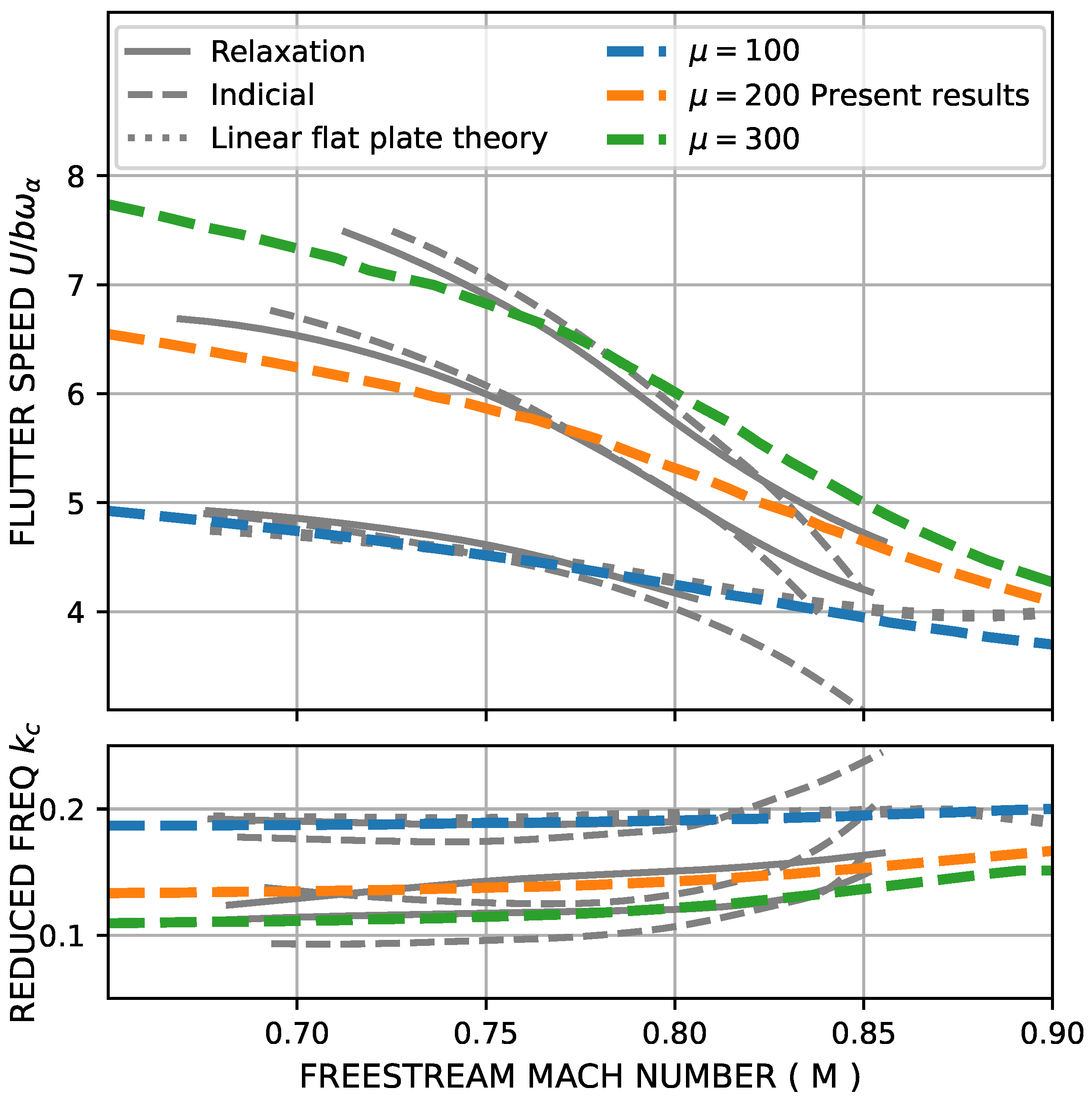
Next, the generalized aerodynamic forces in the Laplace domain are validated by computing flutter velocity and frequency and comparing with other existing methods. Figure 5 presents the flutter speed and the flutter frequency as functions of the Mach number of a flat plate for different mass ratios $\mu$, defined as $\mu =\frac{m_s}{\pi {\rho }_{\infty }{(c/2)}^2}$ (with $m_s$ being the mass of the section per meter). Comparisons with linear theory, as the one used in this work, and with the indicial and relaxation methods [27] are made in the figure. It can be observed that the present method provides the same tendency as the linear theory for the value of $\mu =100$ up to Mach number $0.8$. For higher values of the Mach number, the result of the present method deviates from the strictly linear theory due to the influence of the transonic adjustment here used. The deviation tends to approach to the more exact solutions of the indicial and relaxation methods, demonstrating thus the improvement obtained by the present method in the transonic Mach number range. In the range of Mach number from 0.65 to 0.75, there is also a difference between the present method and the indicial and relaxation methods for values of the mass parameter of $\mu =200$ and $\mu =300$; no reason for this discrepancy has been found so far.

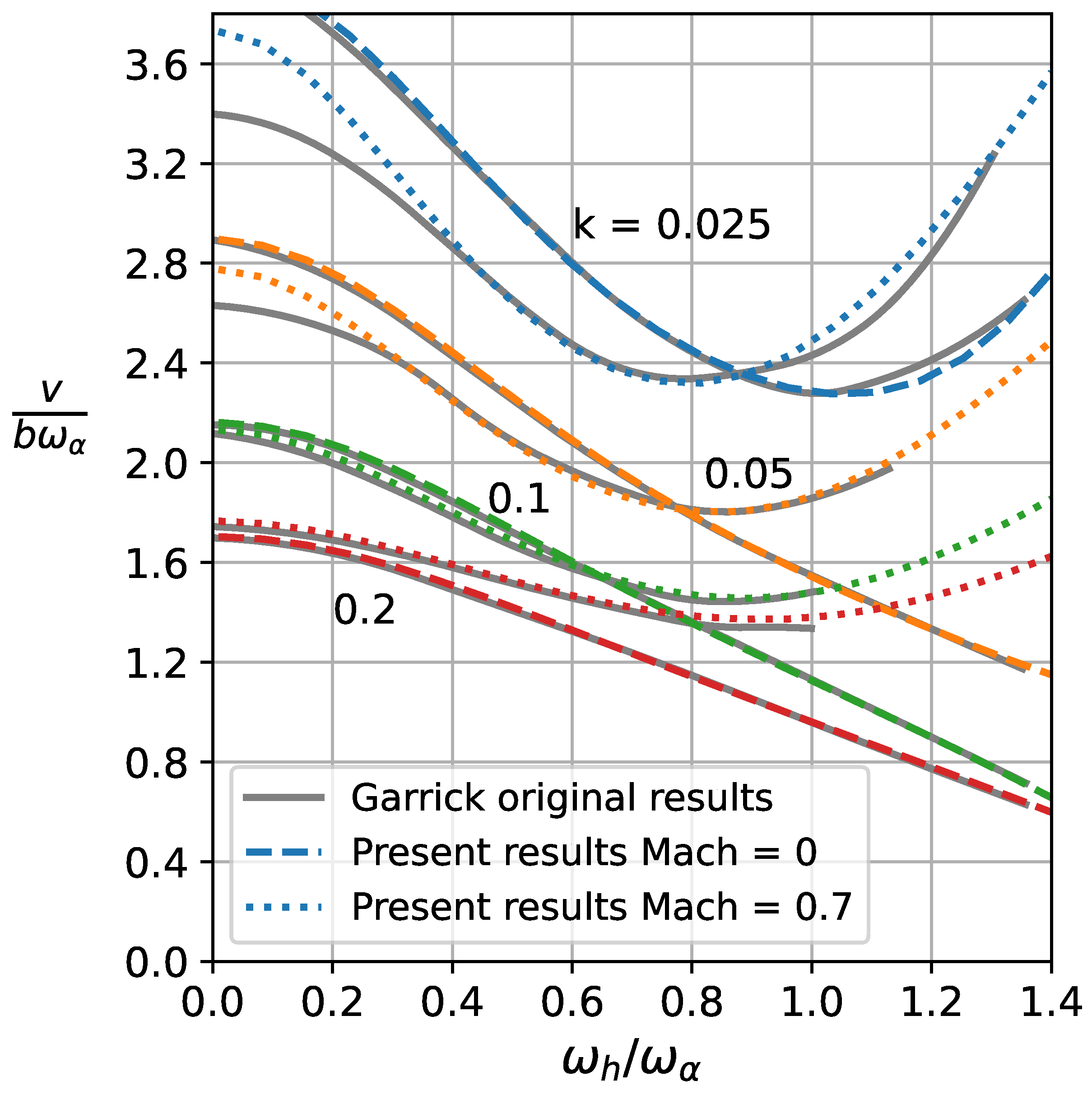
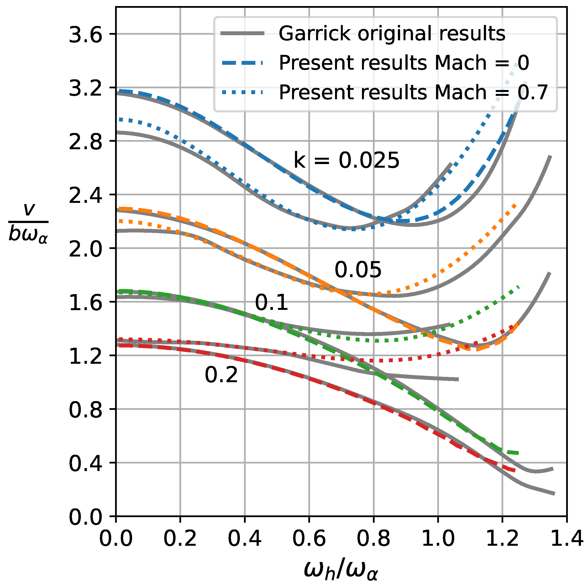
Figure 6 and Figure 7 present the flutter speed as a function of the natural frequency ratio for Mach number 0.0 and 0.7 for two different positions of the elastic axis ${\Lambda }_1=0.0$ and ${\Lambda }_1=-0.2$. In both figures, it can be observed that the agreement between the present method and the results given by Garrick [15] is very good, thus validating the unsteady aerodynamic forces for the subsonic regime.

In order to further compare the obtained results with those of previous authors, the flutter computation for the three degrees of freedom system in the Laplace domain is presented in Figure 8. Comparison is made with the results presented in [25] for the incompressible case and with results obtained from P-K method. The values of the parameters used for the system are shown in

Table 1. Three DOF section parameters for a wing section in incompressible flow.

${\Lambda }_1=-0.4$	${\omega }_h=50$ Hz	$x_{\alpha }=0.2$	$x_{\delta }=0.0125$
$c=0.6$	${\omega }_{\alpha }=100$ Hz	$r_{\alpha }^2=0.25$	$r_{\delta }^2=0.00625$
$\mu =40$	${\omega }_{\beta }=300$ Hz		${\zeta }_{\delta }=0$

. It can be seen that the agreement between this case and Edward’s results at $M_{\infty }=0$ is perfect. The evolution of the system for Mach numbers of $0.4$, $0.6$ and $0.8$ is also presented. The results are close to the ones obtained with the P-K method near the imaginary axis, although the branches become separate far from it. In all the cases, the first root (with lower frequency) associated to the pitching degree of freedom is the one that becomes unstable. When the Mach number is increased, the flutter velocity is reduced, although flutter occurrence is more violent at lower Mach numbers.

It can be seen that the airfoil becomes unstable for all the Mach numbers studied. In order to stabilize it, a control law will be obtained, following the development previously presented. The feedback gain is complex, with its modulus representing the total amount of moment that the actuator would provide, and the angle accounting for the phase between angular velocity of the airfoil and the applied moment.

For a first approach, the phase angle will be fixed, and the gain modulus will be increased with angular velocity. A sweep in phase angle is carried out; the best results are presented in Figure 9 for the incompressible case. The maximum effect of the feedback gain is obtained for a phase angle of 100deg, since applying higher values of the phase angle destabilizes the system.

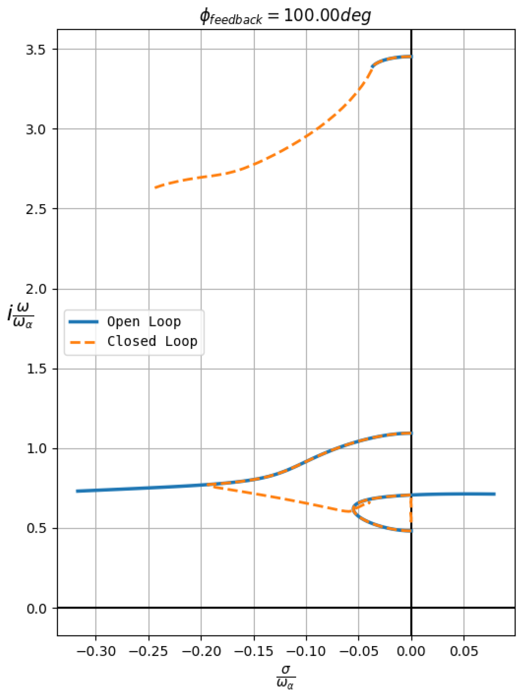
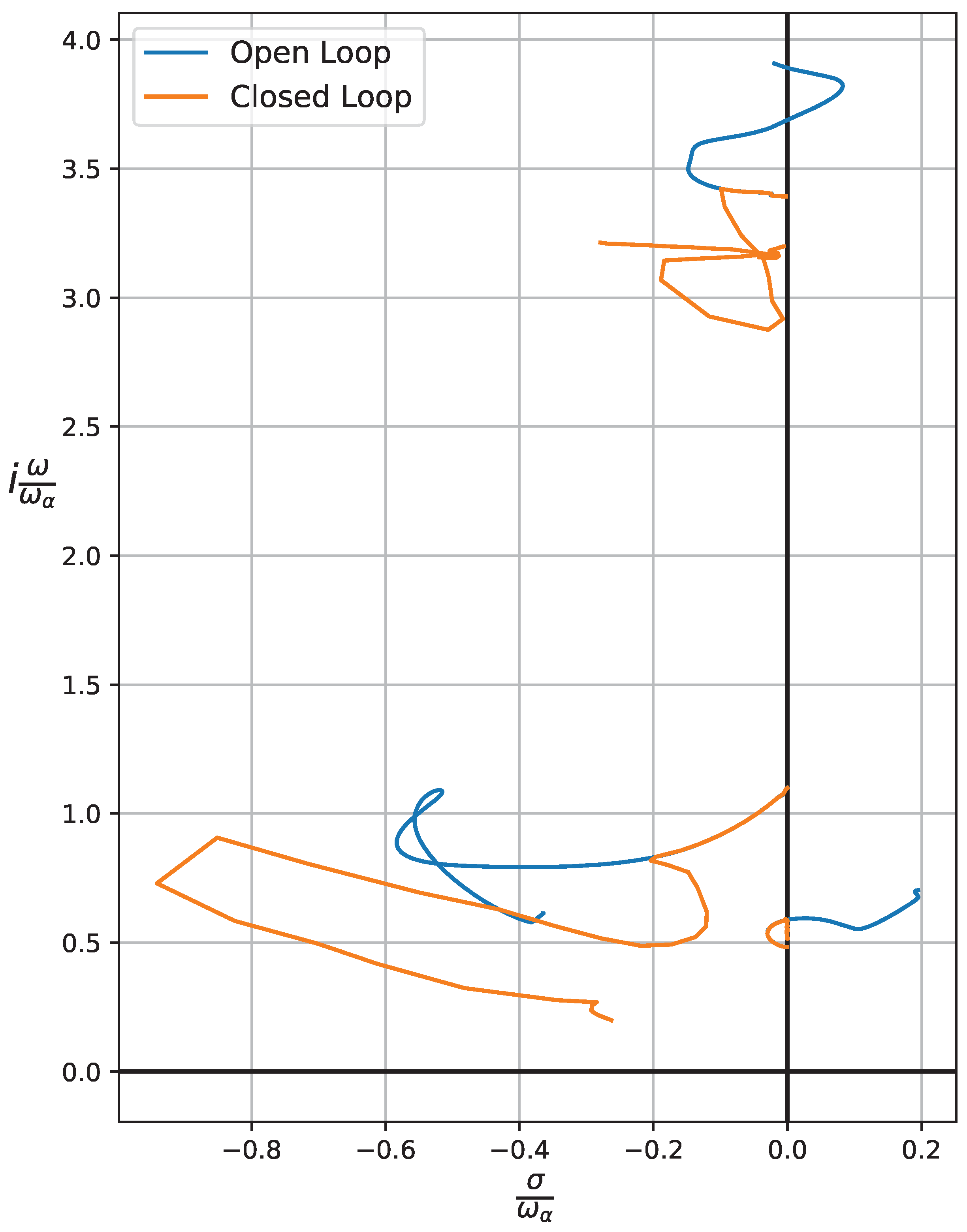
With the optimal phase angle for the feedback gain $\phi =100$ deg, the problem consists of calculating the required gain modulus so as to set the maximum value of the real part of the poles to zero. Figure 10 shows that the system in a closed loop becomes stable, however, forcing the lower branch (plunging mode) to stay in the left side of the imaginary axis, which leads to the torsional mode branch to approach to this axis remaining on the stable side.

Finally, the results for the stabilization of a system in compressible flow are shown. A 3 DOF airfoil with unstable plunging and control surface modes will be used with the parameters shown in

Table 2. Three DOF section parameters for compressible flow.

${\Lambda }_1=0$	${\omega }_h=50$ Hz	$x_{\alpha }=0.2$	$x_{\delta }=0.0125$
$b=1.35$	${\omega }_{\alpha }=100$ Hz	$r_{\alpha }^2=0.25$	$r_{\delta }^2=0.00625$
$c=0.6$	${\omega }_{\beta }=317$ Hz	$\mu =40$	${\zeta }_{\delta }=0$

and speed of sound $a_{\infty }=333$ m/s.

As above, first, the optimal control law is obtained. The main difference with respect to the previous case lies in the fact that now, both the modulus and the phase will vary in the compressible case due to the more complex behavior of this regime. In order to find adequate values, an optimization procedure is carried out. The objective function tends to minimize the required gain modulus while maintaining the system stable. The need to minimize the module is due to the fact that it is directly related to the energy used by the control system. In each step of the optimization, the feedback phase angle from the last iteration is maintained, and a search for the minimum gain module is carried out. Next, the phase is modified, and a new module is obtained. This procedure is repeated until the feedback gain cannot further be reduced.

Figure 11 shows the optimal points computed for each Mach number, and the definite control law obtained by applying a polynomial regression to those points. The control law begins actuating at Mach 0.625, since for smaller values, the system is already stable in an open loop. Then, the modulus and phase vary with the Mach number nonlinearly. The modulus does not increase linearly, since even though it stabilizes the plunging mode, an excessive value tends to destabilize the control surface mode.

Figure 12 shows the poles of the airfoil once the calculated control law was applied. In order to track the aeroelastic modes throughout the branches, the initial steepest descent method must be modified. To ensure that the solution obtained in each iteration corresponds to the adequate branch, a maximum step size in the Laplace plane variable must be fixed, but the Mach number step becomes variable. This maximum step size in the Laplace variable sets the maximum value of the step size for the Mach number. This process accounts for the jumps observed in the presented figure.

It can be seen that system becomes stable for all regimes up to Mach $1.5$. The pole branches are not smooth due to the nonlinearity of the control law. If a more linear control law was developed, the branches would presumably become smoother.

7. Discussion

The objective of this work was to obtain a method for the computation of the unsteady aerodynamic forces in the Laplace domain, which is valid for a wide Mach number range. The method is intended for a wing section and is based on the linearized potential theory. In the transonic regime, the approach is based on an interpolation procedure between the solution for a high subsonic Mach number, for Mach number one and for a low supersonic Mach number. Although it is known that in the transonic range, nonlinearities play an important role, the intrinsic difficulties in the development of appropriate codes and the high computational cost for this case makes the procedure presented in this work an attractive option for the development of control laws for flutter suppression.

The unsteady aerodynamic forces obtained by the present method have been validated in the complete Mach number range with existing solutions in the frequency domain. Flutter computations in the frequency domain, V-g method, and in the Laplace domain (p-method) have also been presented and compared to available methods. Finally, an application for flutter suppression for a system with three degrees of freedom is given, and a control law is obtained.This method thus provides a useful tool for flutter suppression without the need to curve-fit unsteady aerodynamic forces from the frequency domain to the Laplace domain. A control law can be generated using this linear theory and then be tested in a nonlinear transonic code as proposed by Vepa and Kwon [8]. In addition, the unsteady aerodynamic forces obtained by this method can be corrected based on wind tunnel test measurements in the transonic regime as put forward by Baker [7]. Both approaches have been recently appointed for active flutter suppression in the transonic domain.

Further studies for optimization of the control laws and more configurations are currently under investigation.