Some Special Types of Orbits around Jupiter

Abstract

This paper intends to show some special types of orbits around Jupiter based on the mean element theory, including stationary orbits, sun-synchronous orbits, orbits at the critical inclination, and repeating ground track orbits. A gravity model concerning only the perturbations of $J_2$ and $J_4$ terms is used here. Compared with special orbits around the Earth, the orbit dynamics differ greatly: (1) There do not exist longitude drifts on stationary orbits due to non-spherical gravity since only $J_2$ and $J_4$ terms are taken into account in the gravity model. All points on stationary orbits are degenerate equilibrium points. Moreover, the satellite will oscillate in the radial and North-South directions after a sufficiently small perturbation of stationary orbits. (2) The inclinations of sun-synchronous orbits are always bigger than 90 degrees, but smaller than those for satellites around the Earth. (3) The critical inclinations are no-longer independent of the semi-major axis and eccentricity of the orbits. The results show that if the eccentricity is small, the critical inclinations will decrease as the altitudes of orbits increase; if the eccentricity is larger, the critical inclinations will increase as the altitudes of orbits increase. (4) The inclinations of repeating ground track orbits are monotonically increasing rapidly with respect to the altitudes of orbits.

1. Introduction

Jupiter is the most massive planet in the solar system. It is also a gas giant planet. Its mass is 2.5 times the mass of other planets in the solar system. The large size of Jupiter also makes it relatively easy to be observed. As a result, it was discovered very early. Jupiter has been one of the major targets for planetary exploration. However, Jupiter’s powerful magnetosphere and radiation belts are threats to all human spacecraft trying to visit Jupiter. Since the 1970s, several space missions have been launched by NASA, such as Pioneer X, Voyager 1, Galileo, and Juno. However, there is still a long way to go to explore Jupiter. There exist many interesting phenomena that have attracted people to explore for many years, for example, the Great Red Spot, Jupiter’s rings, and atmospheric jet streams. As a gaseous planet, Jupiter cannot be explored by landing like a lithospheric planet. We can only use probes to orbit and enter Jupiter’s atmosphere. Therefore, it is necessary to investigate the orbit dynamics around Jupiter. Weibel et al. [1] researched stable orbits between Jupiter and the Sun. Jacobson [2] investigated the gravity field of Jupiter and the orbits of its Galilean satellites. Colwell et al. [3] studied the exogenic dust ring. Recently, Liu et al. [4,5] discussed the dust in the Jupiter system outside the rings and distribution of Jovian dust ejected from the Galilean satellites. Research about this will surely contribute to the orbit design of space missions.

Investigating the dynamical environments around planets has been the focus for space missions in the past few decades. For this purpose, much research concerning various special artificial satellite orbits around planets have been conducted. Usually, these special types of orbits include stationary orbits, frozen orbits, sun-synchronous orbits, repeating ground-track orbits, and orbits at the critical inclination. The original idea about geostationary orbits was first put up by Clarke [6]. He pointed out that satellites with an altitude of 36,000 km above the equator of the Earth would have the same rotation rates as the Earth and stay stationary relative to an observer on the equator. Therefore, geostationary satellites are often used for the sake of communications and navigations. Four equilibrium solutions for geostationary orbits were shown to exist by Musen & Bailie [7]. Moreover, two of them were stable while the other two were unstable. Lara & Elipe [8] calculated periodic orbits around equilibrium points in the Earth second degree and order gravity field. For Mars, the stationary orbits, also known as areostationary orbits, and the equilibrium points were studied by Liu et al. [9]. The periodic orbits around the equilibrium points were also calculated by Liu et al. [10].

For orbits at the critical inclination, the eccentricity and argument of perigee are invariant on average. The concept of the Earth critical inclination was first introduced by Orlov [11]. Brouwer [12] used canonical transformations to eliminate short-period terms. Coffey et al. gave a geometrical interpretation of the critical inclination for satellites by investigating the averaged Hamilton system [8]. Representatives of orbits at the critical inclination are the Russian Molniya satellites. The combined effects of the critical inclination and the 2:1 mean motion resonance of a Molniya orbit have been intensively studied since then, for example, in [13,14,15,16,17]. Similarly, frozen orbits are characterized by the invariance of average eccentricity and argument of perigee. Frozen orbits are not limited to specific inclinations. They may exist at any inclination. Usually, the argument of perigee is equal to 90 or 270 deg, depending on the sign of the ratio of the harmonic coefficients $J_3$ and $J_2$. Frozen orbits were first proposed by Cutting et al. [18] for orbit analysis of the Earth satellite SEASAT-A. Coffey et al. [19] showed that there exist three families of frozen orbits in the averaged zonal problem up to $J_9$ in the gravity field of an Earth-like planet. The frozen orbits around the moon in the full gravity model were considered by Folta & Quinn [20], and Nie & Gurfil [21]. Some researchers also view orbits at the critical inclination as frozen orbits, for example [19,22].

Sun-synchronous orbits are defined with a precession rate of the orbital plane equal to the revolution angular velocity around the sun. Generally, remote sensing satellites are placed into these orbits. Macdonald et al. [23] used an undefined, non-orientation-constrained, low-thrust propulsion system to consider an extension of the sun-synchronous orbits.

For repeating ground track orbits, the trajectory ground track repeats after a whole number of revolutions within some days. Orbits of this type are widely used to achieve better coverage properties. Lara showed that orbits repeating their ground track on the surface of the Earth were members of periodic-orbit families of the tesseral problem of the Earth artificial satellite [24].

Lei [25] considered the leading terms of the Earth’s oblateness and the luni-solar gravitational perturbations to describe the secular dynamics of navigation satellites moving in the medium Earth orbit and geosynchronous orbit regions. Liu et al. [9] calculated these five types of special orbits around Mars with analytical formulations and numerical simulations. In fact, the gravity field of Mars shares many similarities with that of the Earth. The $J_2$ terms of them are dominant among the harmonic coefficients. However, the $J_2$ term is not as dominant as Earth’s $J_2$. The other first few harmonic coefficients are also strong for Mars: about 1–2 orders of magnitude smaller than $J_2$; for the Earth, the other first few harmonic coefficients are about 3–4 orders of magnitude smaller than $J_2$.

The situation is rather different for Jupiter compared with the Earth and Mars. Due to the difficulty of determining the gravity field of Jupiter, there exist few studies about special types of orbits around Jupiter, as far as we know. However, the situation has greatly improved since Juno’s gravitational measurements were conducted. Iess et al. [26] provided measurements of Jupiter’s gravity harmonics (both even and odd) through precise Doppler tracking of the Juno spacecraft. Moreover, they pointed out a North-South asymmetry, which is a signature of atmospheric and interior flows. Here, we mainly use the results in [26] to build a simplified gravity model of Jupiter. Some harmonic coefficients of the gravity model of the Earth, Mars, and Jupiter can be seen in Table 1.

Table 1. Some harmonic coefficients and their ratios of the Earth, Mars, and Jupiter.

Planet	${\mathit{J}}_2$$\left(\times {10}^{-3}\right)$	${\mathit{J}}_3$$\left(\times {10}^{-6}\right)$	${\mathit{J}}_4\left(\times {10}^{-5}\right)$	${\mathit{J}}_{22}$$\left(\times {10}^{-6}\right)$	${\mathit{J}}_3/{\mathit{J}}_2$$\left(\times {10}^{-3}\right)$	${\mathit{J}}_4/{\mathit{J}}_2\left(\times {10}^{-2}\right)$
Earth ([27])	$1.08263$	$-2.53266$	$-1.61962$	$1.81534$	$-2.3394$	$-1.4960$
Mars ([28])	$1.95545$	$31.4498$	$-1.53774$	$63.0692$	$16.083$	$-0.7864$
Jupiter ([26])	$14.6965$	$0.042$	$-58.661$	$0$	$0.0021378$	$-3.9923$

In this paper, we investigate some special orbits around Jupiter, considering mainly the effect of the non-spherical perturbation of the gravity field.

From Table 1, one can see that the J₂ term is still dominating, J₂ is about 25 times the value of $J_4$, but is ${10}^5$ times bigger than $J_3$. The terms, such as $J_3,J_{21},J_{22},J_5,J_6$ (the values and their uncertainty can be seen in [26]), can be neglected compared with the terms of $J_2$ and $J_4$. Therefore, a good approximation of the gravity model of Jupiter is given by

$$U=\frac{\mu }{r}\left[1-\frac{J_2}{2}{\left(\frac{R}{r}\right)}^2\left(3 {\sin }^2\varphi -1\right)-\frac{J_4}{8}{\left(\frac{R}{r}\right)}^4\left(35{\sin }^4\varphi -30{\sin }^2\varphi +3\right)\right],$$

(1)

where $\mu =G{M}_J$ is the gravitational constant of Jupiter, $\mathrm{G}=6.67428\times {10}^{-11} {\mathrm{m}}^3\cdot \mathrm{k}{\mathrm{g}}^{-1}\cdot {\mathrm{s}}^{-2}$, $M_J$ is the mass of Jupiter, $R$ is the radius of Jupiter, $r$ is the distance of the satellite relative to the center of mass of Jupiter, $\varphi$ is the latitude of the satellite. Equation (1) indicates that the gravity model of Jupiter that we use here is symmetrical with respect to the z-axis. This leads to different characteristics of satellites orbiting around Jupiter and the Earth or Mars. In the next sections, we adopt the gravity model represented by Equation (1) and use it to study some mean features of orbits around Jupiter.

2. Stationary Orbits

Satellites on stationary orbits are well-known for their stationary ground track. Therefore, stationary orbits are preferred for designing communications and navigation satellites. There exist numerous studies on stationary orbits of the Earth and Mars. However, the gravity field of Jupiter is significantly different. In this subsection, we will calculate the stationary orbit of Jupiter and investigate their stability in a spherical coordinate system.

In the spherical coordinates of an inertial frame, $O-r,\lambda ,\varphi$, where $O$ is the center of mass of Jupiter, λ is the jovicentric longitude, r and $\varphi$ are the same as those in Equation (11), and the kinetic energy of the spacecraft can be written as

$$T=\frac{1}{2}({\dot{r}}^2+r^2{\cos }^2\varphi {\dot{\lambda }}^2+r^2{\dot{\varphi }}^2),$$

(2)

where $\dot{r}, \dot{\lambda }, \dot{\varphi }$ are the derivatives with respect to time. From the expressions of T and $U$, one can see that $\lambda$ is a cyclic variable. Let us introduce $q={[r,\lambda ,\varphi ]}^T$, the Lagrangian can be written as $L=T-U$. By Lagrange equations, we have

$$\frac{d}{dt}\left(\frac{\partial T}{\partial \dot{q}}\right)-\frac{\partial T}{\partial q}=\frac{\partial U}{\partial q}.$$

(3)

More precisely, the equations of motion can be presented as follows:

$$\{\begin{array}{l}\ddot{r}-r{\cos }^2\varphi {\dot{\lambda }}^2-r{\dot{\varphi }}^2=-\frac{\mu }{r^2}+\frac{3\mu J_2{R}^2}{2r^4}\left(3{\sin }^2\varphi -1\right)+\frac{5\mu J_4{R}^4}{8r^6}\left(35{\sin }^4\varphi -30{\sin }^2\varphi +3\right),\\ \frac{d}{dt}\left(r^2{\cos }^2\varphi \dot{\lambda }\right)=0,\\ \frac{d}{dt}\left(r^2\dot{\varphi }\right)+\frac{1}{2}{r}^2\sin \left(2\varphi \right){\dot{\lambda }}^2=-\left[\frac{3\mu J_2{R}^2}{2r^3}+\frac{\mu J_4{R}^4}{8r^5}\left(70{\sin }^2\varphi -30\right)\right]\sin 2\varphi .\end{array}$$

(4)

From the second equation of (4), we see that the quantity $r^2{\cos }^2\varphi \dot{\lambda }$ is invariant, which can also be obtained by conservation of the angular momentum along the z-axis. Moreover, the zonal terms of the gravity field only lead to radial and North-South perturbations. The presence of these terms increases the radius of the stationary orbit with respect to the case of a spherical planet with the same mass of Jupiter. When the orbital plane coincides with the equatorial plane, namely $\varphi =0,\stackrel{\cdot }{\varphi }=0$, the vertical perturbation vanishes. In order to find stationary orbits for Jupiter, let $\dot{r}=\ddot{r}=0,\hspace{0.17em}\dot{\lambda }=n_J,\hspace{0.17em}\ddot{\lambda }=0,\hspace{0.17em}\dot{\varphi }=\ddot{\varphi }=0$ in these equations; we get

$$\{\begin{array}{l}{n}_J^2=\frac{\mu }{r^3}+\frac{3\mu J_2{R}^2}{2r^5}-\frac{15\mu J_4{R}^4}{8r^7},\\ \sin 2\varphi =0,\end{array}$$

(5)

or

$$\{\begin{array}{l}-\frac{\mu }{r^2}+\frac{3\mu J_2{R}^2}{2r^4}\left(3{\sin }^2\varphi -1\right)+\frac{5\mu J_4{R}^4}{8r^6}\left(35{\sin }^4\varphi -30{\sin }^2\varphi +3\right)+r{\cos }^2\varphi n_J{}^2=0,\\ \frac{1}{2}{r}^2{n}_J{}^2+\frac{3\mu J_2{R}^2}{2r^3}+\frac{\mu J_4{R}^4}{8r^5}\left(70{\sin }^2\varphi -30\right)=0,\end{array}$$

(6)

where $n_J$ is the rotational angular velocity of Jupiter. One can verify that the left-hand side of the second equation in (6) is always positive when $r$ is larger than $R$. Therefore, we only need to analyze solutions of Equation (5). From the second equation of (5), we see that only one meaningful latitude of the stationary orbit exists, i.e., $\varphi =0$ ($\varphi =\frac{\pi }{2},\pi$ are also roots of $\sin \left(2\varphi \right)=0$, but $\varphi =\frac{\pi }{2}$ makes no sense for stationary orbits, and $\varphi =\pi$ corresponds to a stationary orbit which coincides with that of $\varphi =0$). 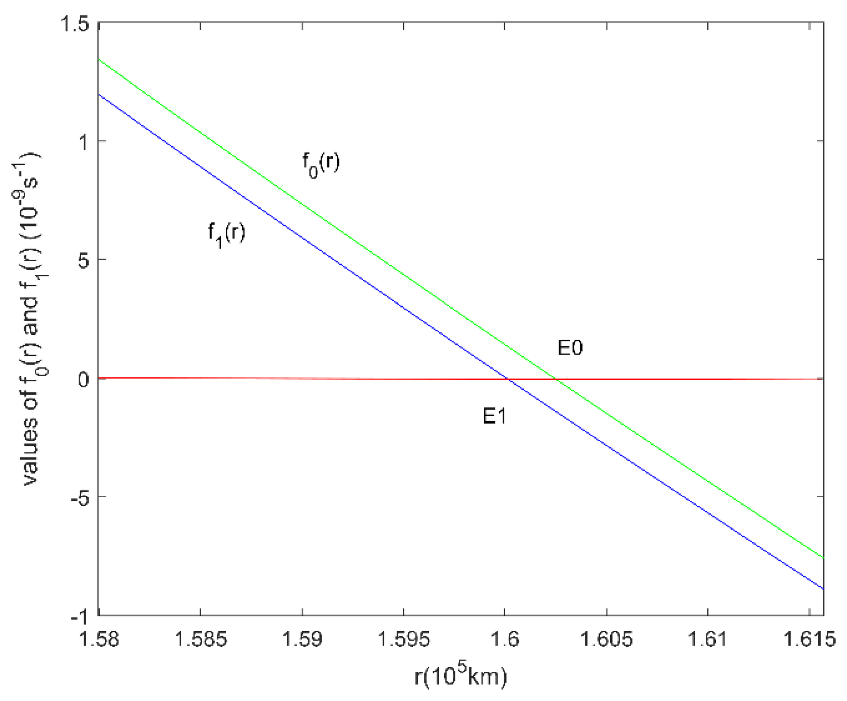Introducing the functions $f_0(r)=\frac{\mu }{r^3}+\frac{3\mu J_2{R}^2}{2r^5}-\frac{15\mu J_4{R}^4}{8r^7}-n_J^2$ and $f_1(r)=\frac{\mu }{r^3}-n_J^2$, the variations of $f_0(r),\hspace{0.17em}{f}_1(r)$, with respect to $r$, can be seen in the following Figure 1.

Figure 1. Variations of $f_0(r),\hspace{0.17em}{f}_1(r)$ as $r$ increases from $2.2R$ to $2.3R$.

It can be proved that $f_0(r)$ vanishes at two real positive values of $r$, but only one of them is bigger than $R$. This solution, which is given by $r_0=2.2414R=1.6024\times {10}^8 \mathrm{m}$, is denoted by E0 in Figure 1. If the perturbation due to the non-spherical gravity field is not considered, one can find that the radius for stationary orbits is about $2.2381R$, which corresponds to the point E1. Therefore, the existence of the $J_2$ and $J_4$ terms increase the altitude of the stationary orbit.

To study the stability of the stationary orbits under small perturbations, we mainly used the epicyclic theory (Murray & Dermott [29]). We can denote by the constant $h$, the value taken by $r^2{\cos }^2\varphi \dot{\lambda }$ for some given initial conditions. Assuming that the deviations from the stationary orbits are small and writing $r=r_0\left(1+\epsilon \right)$, Equation (4) can be linearized as follows (Murray & Dermott [29], Section 11 of Chapter 6):

$$\{\begin{array}{c}\begin{array}{c}\ddot{\epsilon }+\left(3{\alpha }_1+{\alpha }_2\right)\epsilon =0,\\ \ddot{\varphi }+\left({\alpha }_1+{\beta }_2\right)\varphi +{\beta }_1=0,\end{array}\\ \stackrel{\cdot }{\lambda }-\frac{h}{r_0{}^2{\left(1+\epsilon \right)}^2{\cos }^2\varphi }=0\end{array}$$

(7)

where ${\alpha }_1=-\frac{1}{r_0}\frac{\partial U}{\partial r}(r_0,0)$, ${\alpha }_2=-\frac{{\partial }^{2}U}{\partial r^2}(r_0,0)$, ${\beta }_1=-\frac{1}{r_0{}^2}\frac{\partial U}{\partial \varphi }(r_0,0)$, and ${\beta }_2=-\frac{1}{r_0{}^2}\frac{{\partial }^{2}U}{{\partial }^2\varphi }(r_0,0)$. By solving Equation (7), the analytical approximate expressions of $\epsilon ,\hspace{0.17em}\varphi ,\hspace{0.17em}\lambda$ can be formulated as [29]

$$\{\begin{array}{l}\epsilon =e\cos k_{1}t,\\ \varphi =-\frac{{\beta }_1}{{\alpha }_1+{\beta }_2}+i\cos k_{2}t,\\ \lambda =\sqrt{{\alpha }_1}t-\frac{2\sqrt{{\alpha }_1}}{k_1}e\sin k_{1}t,\end{array}$$

(8)

where $k_1^2=3{\alpha }_1+{\alpha }_2$, $k_2^2={\alpha }_1+{\beta }_2$, $i$ is the inclination, and $e$ is the eccentricity of the orbit. Note that the average of $\dot{\lambda }$ is $\sqrt{{\alpha }_1}$. Let us set $k_3=\sqrt{{\alpha }_1}.$ The first two equations in (7) or (8) show that the radial and North-South motions are uncoupled. Using the expression (1), we can get a precise form of the three frequencies $k_1,k_2,k_3$ [29]:

$$\{\begin{array}{l}{k}_1{}^2=\frac{\mu }{r_0{}^3}\left[1-\frac{3}{2}{J}_2{\left(\frac{R}{r_0}\right)}^2+\frac{45}{8}{J}_4{\left(\frac{R}{r_0}\right)}^4\right],\\ k_2{}^2=\frac{\mu }{r_0{}^3}\left[1+\frac{9}{2}{J}_2{\left(\frac{R}{r_0}\right)}^2-\frac{75}{8}{J}_4{\left(\frac{R}{r_0}\right)}^4\right],\\ k_3{}^2=\frac{\mu }{r_0{}^3}\left[1+\frac{3}{2}{J}_2{\left(\frac{R}{r_0}\right)}^2-\frac{15}{8}{J}_4{\left(\frac{R}{r_0}\right)}^4\right].\end{array}$$

(9)

Therefore, the satellites will oscillate in the radial and North-South directions with frequencies $k_1$ and $k_2$, respectively. Moreover, the mean motion frequency, $k_3$, in the West-East direction is larger than in the Keplerian case. Namely, for a given semi-major axis, the satellite moves faster than the rate expected at that location in the Keplerian case. In the following, we give some numerical examples to illustrate the above characteristics.

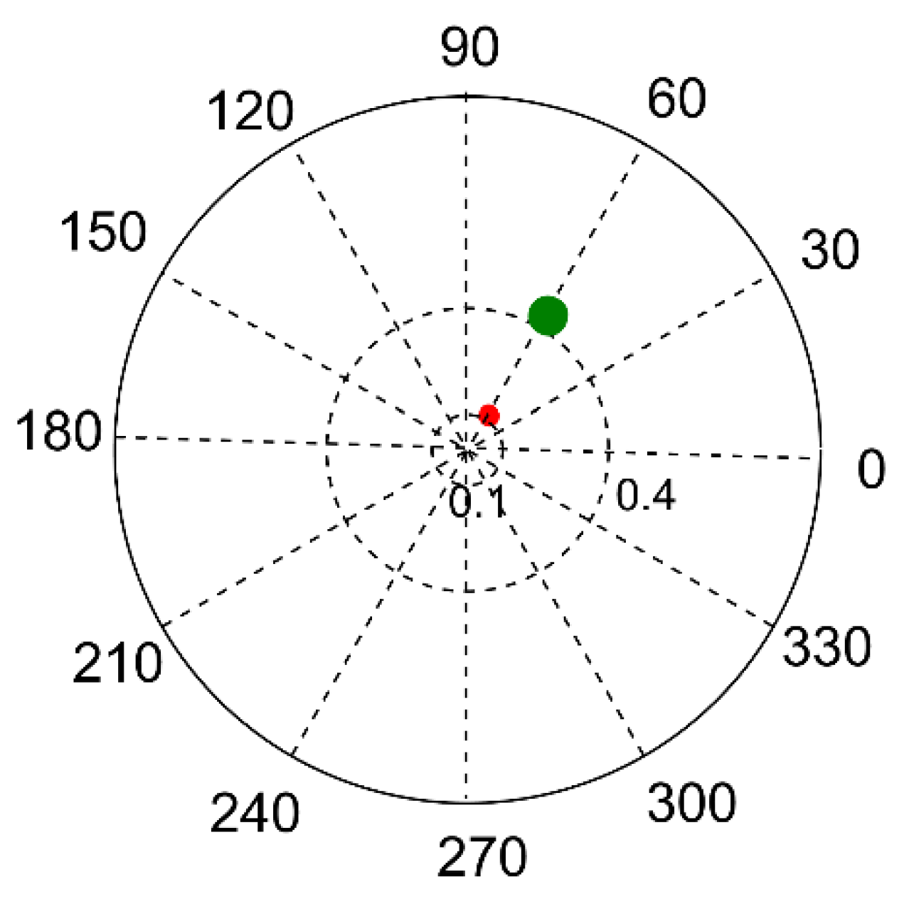
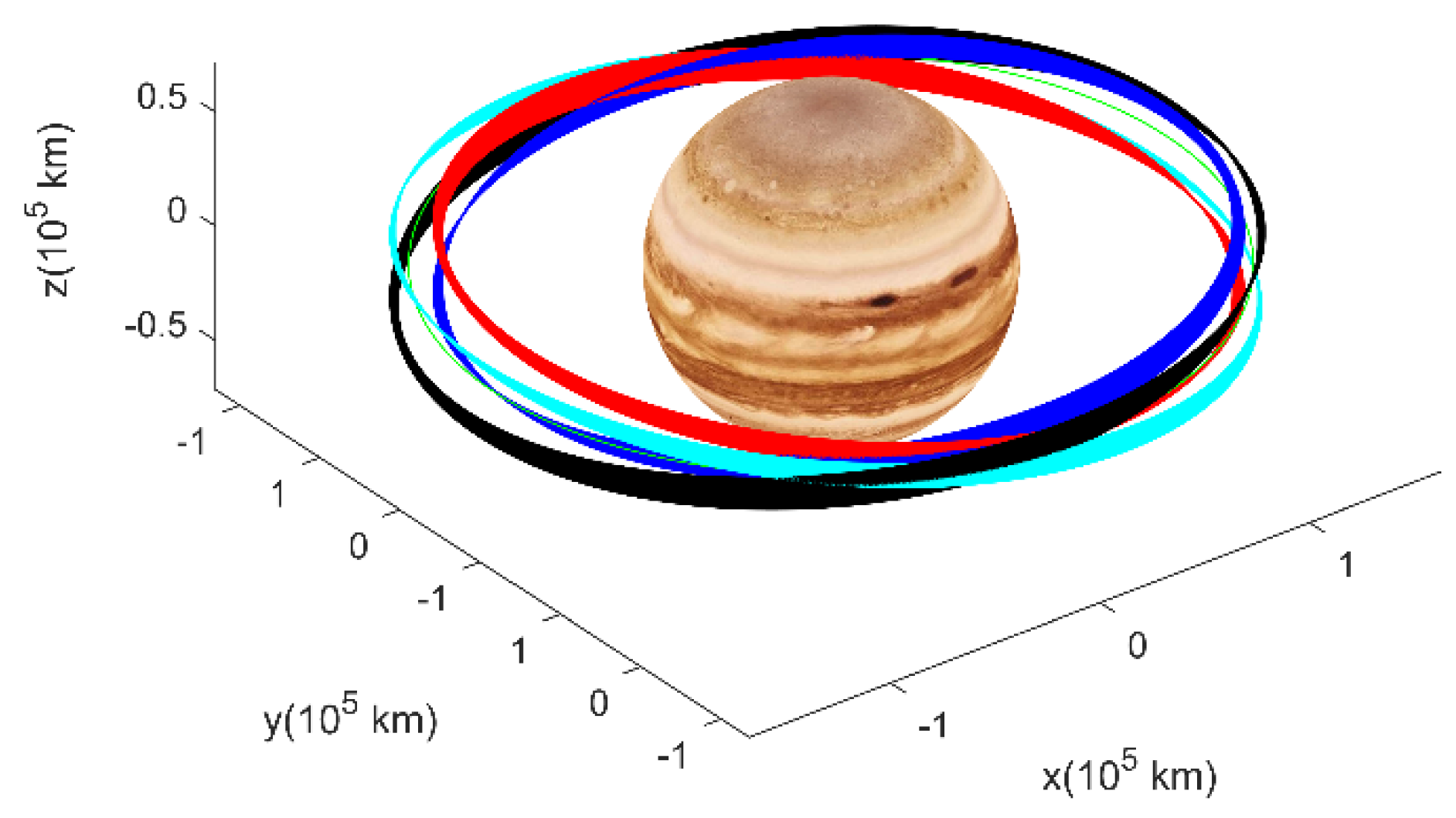
We computed the evolution of $r$, $\varphi$, and $\lambda$ when we selected initial values of $r$ and $\varphi$ close to r₀ and 0, respectively. Figure 2 shows a stationary orbit and four orbits obtained from $r=0.99r_0,\hspace{0.17em}\varphi =\pm 0.1$ deg and $r=1.01r_0,\hspace{0.17em}\varphi =\pm 0.1$ deg. We can see that these four disturbed orbits are no longer periodic. This can be explained by using Equation (9). Due to the presence of the terms that contain $J_2$ and $J_4$, the three frequencies are usually not equal or even commensurable. 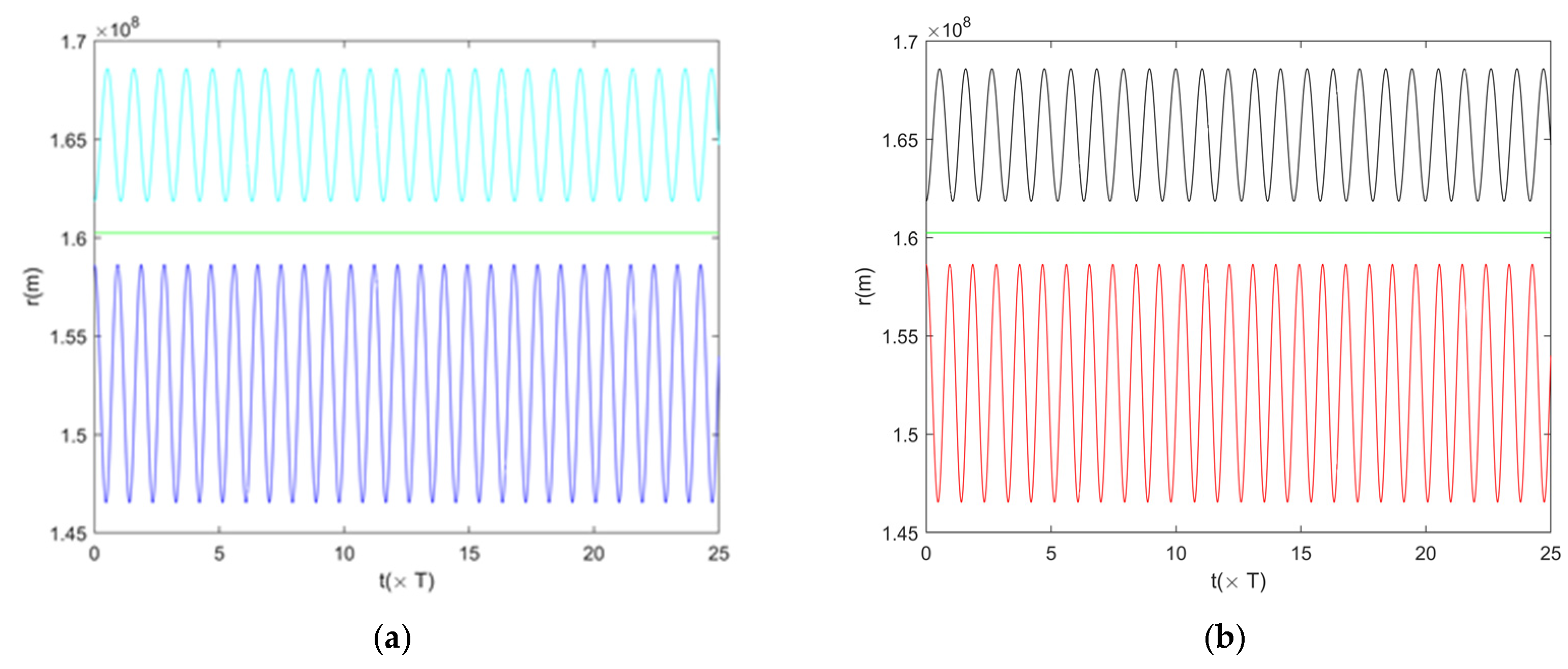Figure 3 illustrates that the satellite oscillates in the radial and North-South directions. On the other hand, the satellite on stationary orbits does not drift in these directions. It only moves with a constant $\dot{\lambda }$ along the orbit. Therefore, the drift of longitude would not occur for satellites on stationary orbits since only zonal harmonics are taken into account in the gravity model. Furthermore, there are no significant differences between points on the stationary orbit. As a result of the symmetry of the gravity field, it can be concluded that the points on stationary orbits are degenerate equilibrium points. Here, an equilibrium point is degenerate if, and only if, the matrix of the linearized equation for (4) is degenerate. This is the major difference with respect to stationary orbits of other planets, such as the Earth and Mars. For the Earth and Mars, there exist four equilibrium points on stationary orbits, among which two are stable and the other two are unstable.

Figure 2. Orbits around Jupiter: green—stationary orbits; red—$r=0.99r_0$, $\varphi =-0.1$ deg; blue—$r=0.99r_0$ and $\varphi =0.1$ deg; cyan—$r=1.01r_0$ and $\varphi =-0.1$ deg; black—$r=1.01r_0$ and $\varphi =0.1$ deg.

Figure 3. (a,b) Variations of orbital radius ($r$), (c,d) drift of longitude ($\mathsf{\Delta }\lambda$), (e,f) evolution of latitude ($\varphi$): green—stationary orbits; red, $r=0.99r_0$ and $\varphi =-0.1$ deg; blue—$r=0.99r_0$ and $\varphi =0.1$ deg; cyan—$r=1.01r_0$ and $\varphi =-0.1$ deg; black—$r=1.01r_0$, $\varphi =0.1$ deg, and $T$ is a Jovian day.

In the following, we show that the effects of third bodies, the Jovian ring and the magnetic field of Jupiter, are negligible compared to those of the $J_2$ and $J_4$ terms.

Based on the data of the Sun and moons around Jupiter (see for example, [30]), one can calculate the maximal ratio of the disturbed acceleration ($a_d$) and central gravity acceleration ($a_m$) for satellites on stationary orbits, which is achieved when the satellite, Jupiter, and the third body are in a straight line. Therefore, the maximal ratio can be calculated as [31]

$${\left(\frac{a_d}{a_m}\right)}_{\max }=2\frac{m}{M_J}{\left(\frac{r_0}{\rho }\right)}^3,$$

(10)

where $m$ is the mass of the third body, and $\rho$ is the distance between Jupiter and the third body. Values of the maximum ratio (109) for different bodies are reported in Table 2. Since the $J_4$ term of Jupiter is 100 times bigger than the ratio of acceleration for Io (which gives the highest value among the Galilean satellites), it is reasonable to ignore these effects when investigating the qualitive character of stationary orbits on short time scales. To verify the validity of these solutions, we use the numerical integration method to see the effect of the Galilean moon Io in 800 Jovian days. The orbital elements $\left(a,e,i,\mathsf{\Omega },\omega ,M\right)$ of Io that we adopt here are taken from the 10th China Trajectory Optimization Competition, i.e., $\left(\begin{array}{l}422\text{,}029.687\mathrm{km}\hfill \end{array},0.004308,0.04\mathrm{deg},-79.64\mathrm{deg},37.991\mathrm{deg},4.818\mathrm{deg}\right).$ Calculation results show that the drift of longitude ($\mathsf{\Delta }\lambda$) for the satellite on stationary orbits is less than 0.1 deg in 800 Jovian days. The inclination changes no more than $1.0\times {10}^{-4}$ deg. The oscillation of the semi-major axis is less than 0.13% of the obital radius. However, it should be noted that the obtained solutions may not be correct on long time scales.

Table 2. The disturbing acceleration due to the third body.

The Third Body	$\mathit{m}/{\mathit{M}}_{\mathit{J}}\left(\times {10}^{-5}\right)$	$\mathit{\rho }/{\mathit{r}}_0$	${\left({\mathit{a}}_{\mathit{d}}/{\mathit{a}}_{\mathit{m}}\right)}_{\mathbf{max}}\left(\times {10}^{-6}\right)$
Sun ([32])	$1.0473\times {10}^8$	4856.8	0.01823
Io ([30,32])	4.7047	2.6311	5.20000
Europa ([30,32])	2.5283	4.1868	0.68904
Ganymede ([30,32])	7.8056	6.6775	0.52379
Callisto ([30,32])	5.6673	11.7511	0.06989

The Jovian main ring is about 6440 km wide and probably less than 30 km thick. We denote this width by $w$. Moreover, the distance, $d$, of the ring from the center of mass of Jupiter is about 122,500 km, and the mass, $m_r$, is about 1.0×10¹³ kg [32].

For satellites on stationary orbits with position $r_s$, the gravitational acceleration due to the Jovian main ring can be calculated as

$$F_r=G{\displaystyle \int {\displaystyle \int {\displaystyle {\int }_{ring}\frac{\left(r\left(\mathsf{{\rm P}}\right)-r_s\right)\rho (\mathsf{{\rm P}})dV}{|r\left(\mathsf{{\rm P}}\right)-r_s{|}^3}}}},$$

(11)

where $r\left(\mathsf{{\rm P}}\right),\rho \left(\mathsf{{\rm P}}\right)$ denote the position vector and the density, respectively, which depend on the position of a point, $\mathsf{{\rm P}}$, belonging to the ring. We can see that

$$\begin{gathered} |r(\mathsf{{\rm P}})-r_s|\ge r_0-d-w\approx 160\text{,}240-122\text{,}500-6440\approx 0.4378R, \\ \left|F_r\right|\le \frac{G{m}_r}{{\left(0.4378R\right)}^2}. \end{gathered}$$

Note that $\frac{G{m}_r}{{\left(0.4378R\right)}^2}/\left(\frac{G{M}_J}{r_0{}^2}\right)=\frac{m_r}{M_J}\cdot {\left(\frac{r_0}{0.4378R}\right)}^2\approx \frac{1.0\times {10}^{13}}{1.9\times {10}^{27}}\cdot {\left(\frac{2.2414}{0.4378}\right)}^2\approx 1.3795\times {10}^{-13}$, which is far smaller than $J_2$ and $J_4$ terms. Therefore, the effects of the Jovian main ring on stationary orbits can be neglected.

Another perturbation that may affect stationary orbits is the magnetic field of Jupiter when the satellite is charged. Here, we briefly analyze the effects under some assumptions. The magnetic field of Jupiter near stationary orbits when exterior terms are neglected can be written as

$$B\left(r,\varphi ,\lambda \right)=-\nabla V\left(r,\varphi ,\lambda \right),$$

(12)

where

$$V=R{\displaystyle \sum _{l=1}^{\infty }{\displaystyle \sum _{m=1}^l{\left(\frac{R}{r}\right)}^{l+1}}}\left[g_{l,m}\cos \left(m\lambda \right)+h_{l,m}\sin \left(m\lambda \right)\right]P_l^m\left(\cos \varphi \right).$$

(13)

Here, $g_{l,m}$ and $h_{l,m}$ are the geomagnetic Gauss coefficients (their values can be found in [33,34]), and $P_l^m(\cos \varphi )$ is the normalized Legendre function. The acceleration due to the Lorentz force is

$$F_L=\frac{q}{m}\left(\dot{r}-\omega \times r\right)\times B\left(r,\varphi ,\lambda \right),$$

(14)

where $q=4\pi {\epsilon }_0\mathsf{\Phi }s$,${\epsilon }_0=8.854187817\times {10}^{-12} \mathrm{F}\cdot {\mathrm{m}}^{-1}$ is the vacuum permittivity, $\mathsf{\Phi }$ is the surface potential of satellites, $s$ is the radius of the satellite, $\omega$ is the angular velocity vector of Jupiter. For a charged satellite with $\mathsf{\Phi }=500 \mathrm{V}$ (an in-depth study of the effect of spacecraft charging at Jupiter can be found in [35]), $s=10 \mathrm{m}$, and m = 100 kg, we have $q=5.5633\times {10}^{-7}\mathrm{C}$ and $\left|F_L\right|\le 1.14\times {10}^{-8}\mathrm{N}$. The Lorentz force compared with the lowest order of gravity provides the ratio

$$\frac{{|\mathrm{F}}_L|}{\left|G_0\right|}=\frac{\left(n-n_J\right)Bq{r}^3}{GMm}\approx 2.3\times {10}^{-11}$$

This ratio is also far smaller than $J_2$ and J₄. Therefore, it can be concluded that the effects of Lorentz forces on a satellite can be neglected.

3. Sun-Synchronous Orbits

The oblate nature of the primary body can lead to a secular variation of the ascending node of the orbit. However, we can use the orbit perturbations to keep the orientation of the Sun line direction fixed with respect to the orbital plane (for example, perpendicular to it) during one revolution of Jupiter around the Sun.

Based on the mean element theory, the mean nodal precession rate coming from the secular perturbations of the first and second order [36,37] can be described as

$$\begin{array}{l}\stackrel{.}{\mathsf{\Omega }}=-\frac{3n{J}_2{R}^2}{2a^2{(1-e^2)}^2}\cos i-\frac{9n{J}_2^2{R}^4}{4p^4}\cos i\{\frac{3}{2}+\frac{e^2}{6}+\sqrt{1-e^2}-{\sin }^{2}i\left(\frac{5}{3}-\frac{5e^2}{24}+\frac{3}{2}\sqrt{1-e^2}\right)\\ -\frac{35J_4}{18J_2^2}\left[\frac{6}{7}+\frac{9e^2}{7}-{\sin }^{2}i\left(\frac{3}{2}+\frac{9e^2}{4}\right)\right]\}.\end{array}$$

(15)

For sun-synchronous orbits, the mean nodal precession rate is equal to the mean motion of Jupiter orbiting around the Sun ($n_s$). Thus, we get the following equation:

$$g(\cos i)={\mathsf{\Gamma }}_1{\cos }^{3}i+{\mathsf{\Gamma }}_2\cos i+{\mathsf{\Gamma }}_3=0,$$

(16)

where

$${\mathsf{\Gamma }}_1=\frac{9n{J}_2^2{R}^4}{4p^4}\left[\frac{5}{3}-\frac{5}{24}{e}^2+\frac{3}{2}\sqrt{1-e^2}-\frac{35J_4}{6J_2^2}\left(\frac{1}{2}+\frac{3}{4}{e}^2\right)\right],$$

(17)

$${\mathsf{\Gamma }}_2=\frac{3n{J}_2{R}^2}{2p^2}\left\{1+\frac{3J_2{R}^2}{2p^2}\left[-\frac{1}{6}+\frac{3e^2}{8}-\frac{1}{2}\sqrt{1-e^2}+\frac{5J_4}{2J_2^2}\left(\frac{1}{2}+\frac{3e^2}{4}\right)\right]\right\},$$

(18)

$${\mathsf{\Gamma }}_3=n_s.$$

(19)

Here, we remark that in Equations (17) and (18), $p$ is equal to a(1−e²).

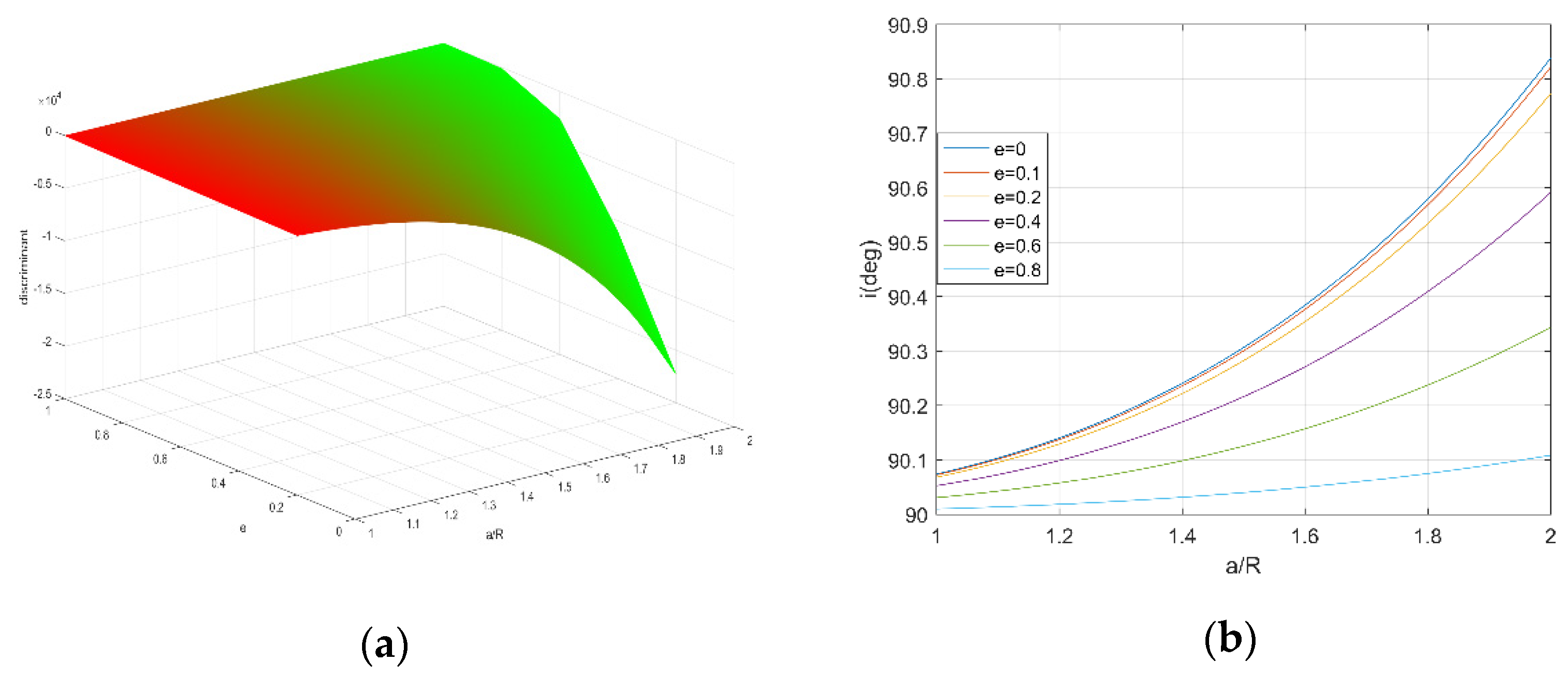
First, setting $x=\cos i$, we note that the equation $g\left(x\right)=0$ has three real roots if the discriminant satisfies the following inequality:

$$\mathsf{\Delta }=-\left(\frac{{\mathsf{\Gamma }}_3^2}{4{\mathsf{\Gamma }}_1^2}+\frac{{\mathsf{\Gamma }}_2^3}{27{\mathsf{\Gamma }}_1^3}\right)\ge 0.$$

(20)

Then, it is also necessary to avoid impact with Jupiter. However, the surface of Jupiter cannot be unambiguously defined since it is a gas giant. The critical perijovian distance, $d_c$, is usually much larger than the radius of Jupiter, $R$, due to radiation safety issues. However, let us take for convenience $d_c=R$, so that the semi-major axis and eccentricity have to satisfy

$$d_c=R<a\left(1-e\right).$$

(21)

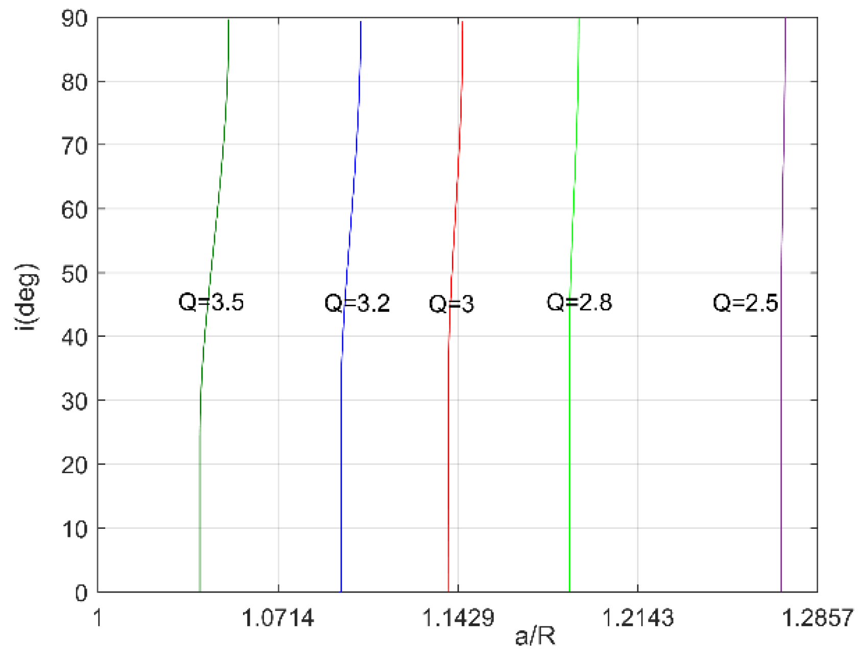
The variation of the discriminant with respect to $a$ and e is shown in Figure 4a. We see that the discriminants are always negative for $a\in [R,2R]$ and $e\in [0,1-\frac{R}{a}]$, therefore, it can be concluded that there usually exists one meaningful inclination for sun-synchronous orbits when the semi-major axis and eccentricity are given. The inclinations for different semi-major axis and eccentricities are shown in Figure 4b. It was shown that the inclination monotonically increases with respect to the semi-major axis. For the same semi-major axis, the inclination decreases as the eccentricity increases. Moreover, the inclinations with the same altitude ratio, $a/R$, are relatively smaller than those of near-Earth sun-synchronous orbits.

Figure 4. (a) Variation of the discriminant with respect to $a$ and $e$; (b) variations of the inclination $i$ as the semi-major axis a increases from $R$ to $2R$.

For satellites on sun-synchronous orbits with medium altitude, perturbations from the gravity of the third body are usually smaller compared to satellites on stationary orbits. However, the risk coming from the Jupiter rings and the magnetic field may increase greatly.

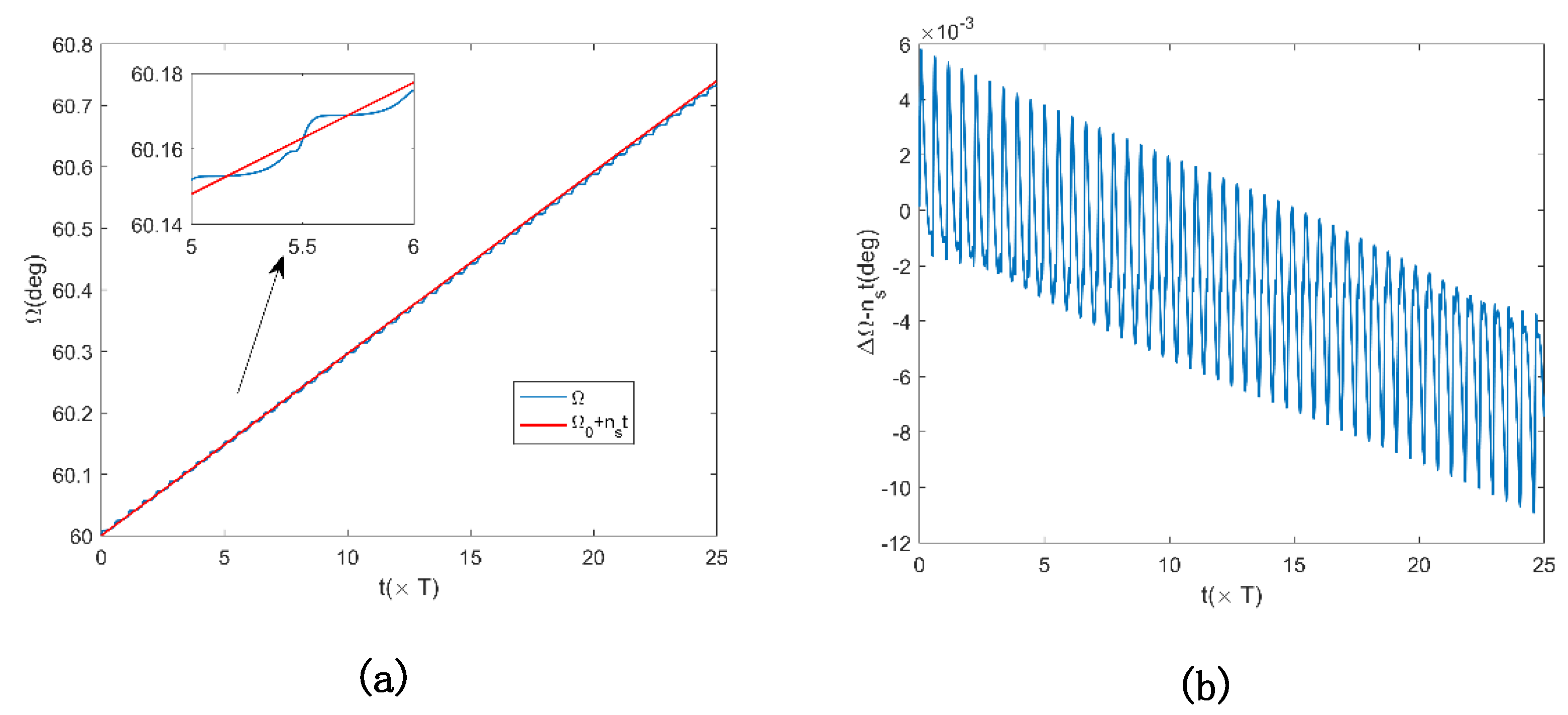
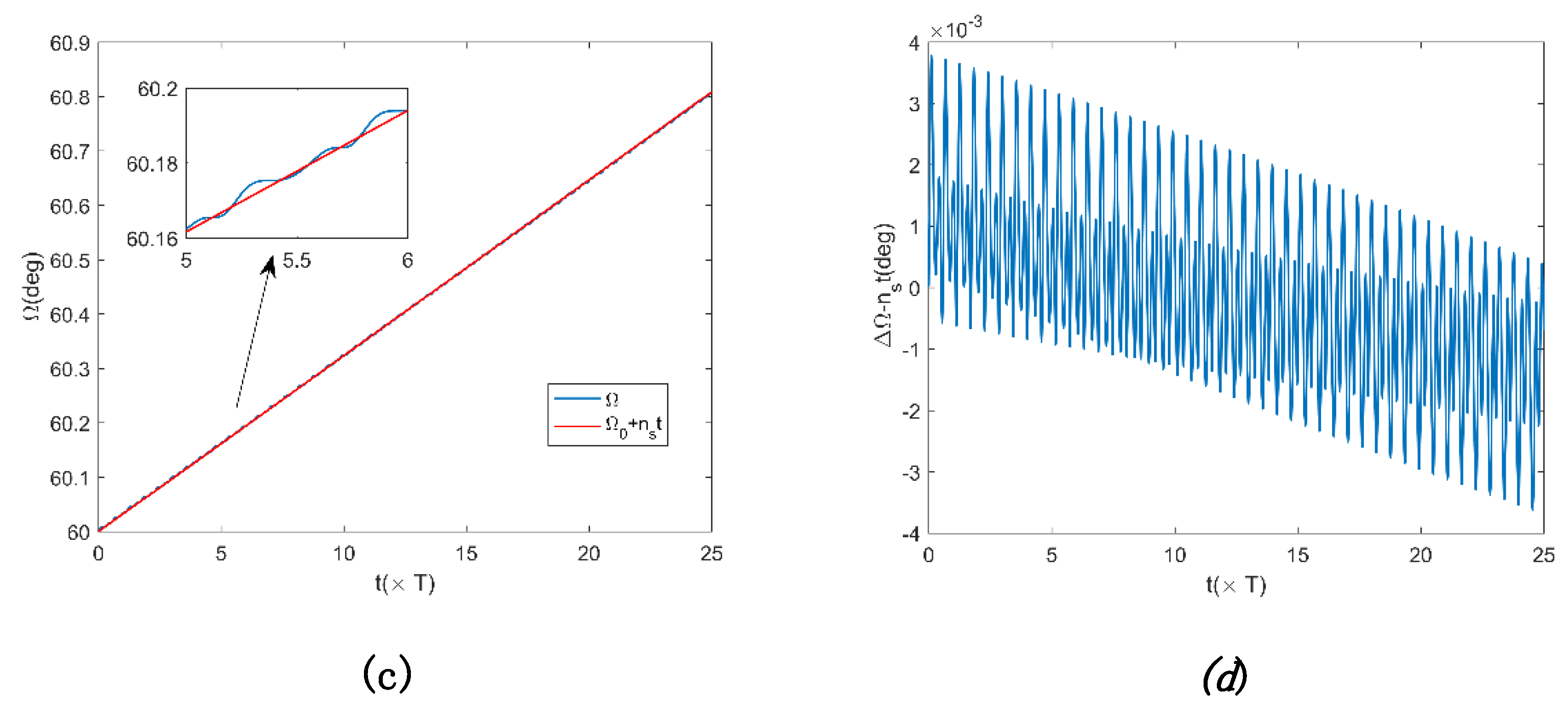
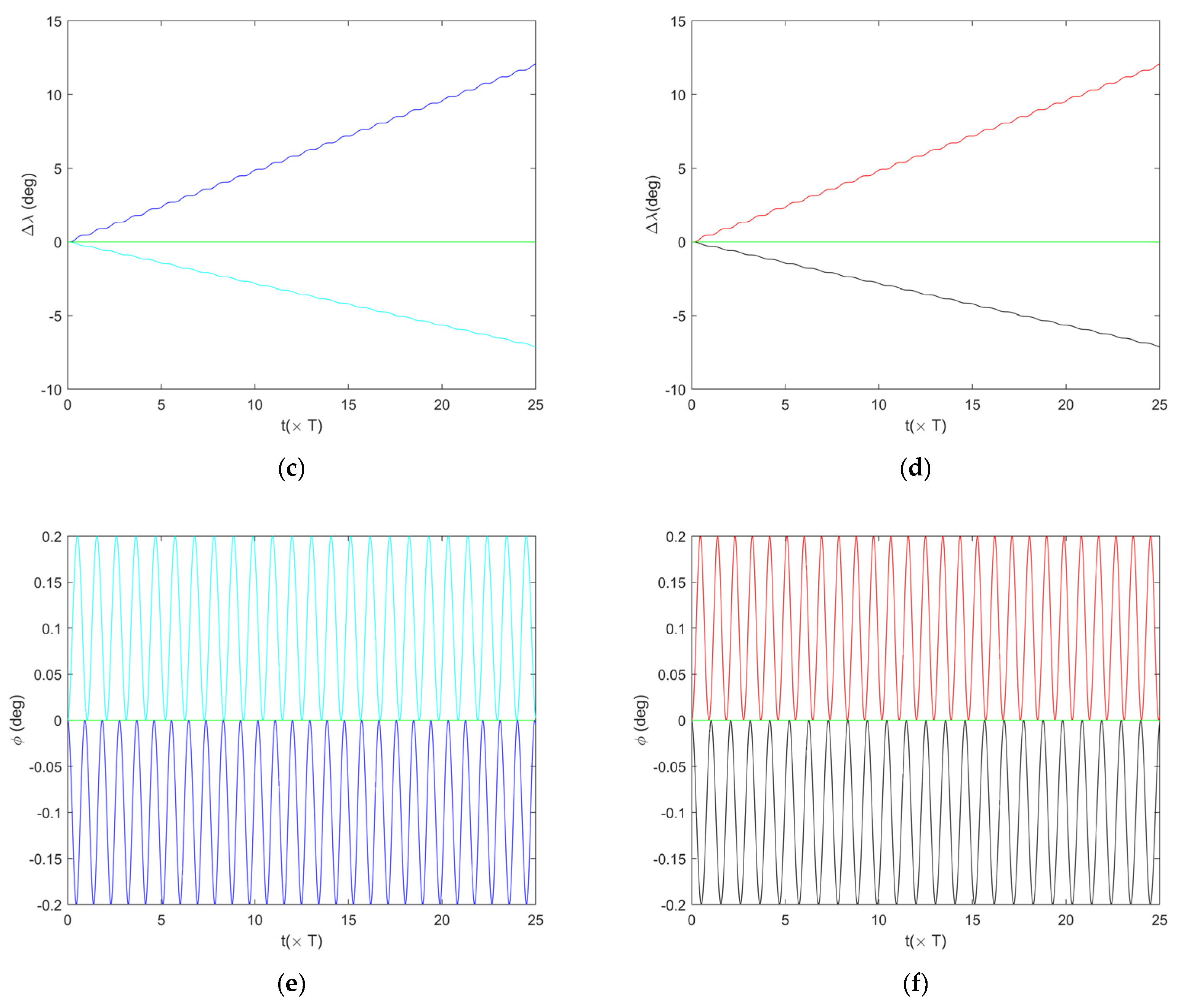
For sun-synchronous orbits, when $a=1.4373R=102\text{,}755.451$ km and $e=0.4$, we have $i=90.183$ deg; when $a=1.5308R=109\text{,}439.953$ km and $e=0.1$, the corresponding inclination is 90.321 deg. The evolution of $\mathsf{\Omega }$ and of the difference between $\mathsf{\Delta }\mathsf{\Omega }$ and $n_{s}t$ over 25T for these two cases are presented in Figure 5. In the first case, this difference is about 0.018 deg; and in the second case, it is about 0.008 deg.

Figure 5. Evolution of $\mathsf{\Omega }$ and difference between $\mathsf{\Delta }\mathsf{\Omega }=\mathsf{\Omega }-{\mathsf{\Omega }}_0$ and $n_{s}t$ over $25T$, where $T$ is a Jovian day, ${\mathsf{\Omega }}_0=60$ deg is the initial condition (the blue curve was indeed obtained by numerical integration of osculating elements). (a) Evolution of $\mathsf{\Omega }$ for $a=102\text{,}755.451$ km, $i=90.183$ deg. (b) Difference between $\mathsf{\Delta }\mathsf{\Omega }$ and $n_{s}t$ for $a=102\text{,}755.451$ km, $e=0.4$, $i=90.183$ deg. (c) Evolution of for $a=109\text{,}439.953$ km, $e=0.1,$ $i=90.321$ deg. (d) Difference between $\mathsf{\Delta }\mathsf{\Omega }$ and $n_{s}t$ for $a=109\text{,}439.953$ km, $e=0.1,$ $i=90.321$ deg.

4. Orbits with Critical Inclination

The variations of the eccentricity and the argument of perijove are mainly caused by the equatorial bulge of Jupiter. These usually produce negative effects on space missions to Jupiter. However, we can choose orbits with critical inclinations to avoid these disadvantages.

According to the mean element theory, the mean variation rate of $\omega$ caused by perturbations of the first and second order [36,37] can be formulated as follows:

$$\begin{array}{l}\dot{\omega }=-\frac{3n{J}_2{R}^2}{2a^2\left(1-e^2\right)}\left(\frac{5}{2}{\sin }^{2}i-2\right)+\frac{9n{J}_2^2{R}^4}{p^4}\{4+\frac{7e^2}{12}+2\sqrt{1-e^2}-{\sin }^{2}i\left(\frac{103}{12}+\frac{3e^2}{8}+\frac{11}{2}\sqrt{1-e^2}\right)\\ +{\sin }^{4}i\left(\frac{215}{48}-\frac{15}{32}{e}^2+\frac{15}{4}\sqrt{1-e^2}\right)-\frac{35J_4}{18J_2^2}\left[\frac{12}{7}+\frac{27e^2}{14}-{\sin }^{2}i\left(\frac{93}{14}+\frac{27e^2}{4}\right)+{\sin }^{4}i\left(\frac{21}{4}+\frac{81e^2}{16}\right)\right]\}.\end{array}$$

(22)

To keep the invariance of the mean argument of perijove, we set $\dot{\omega }=0.$ Therefore, we obtain the following equation

$${\mathsf{\Gamma }}_4{\sin }^{4}i+{\mathsf{\Gamma }}_5{\sin }^{2}i+{\mathsf{\Gamma }}_6=0,$$

(23)

where

$${\mathsf{\Gamma }}_4=\frac{9n{J}_2^2{R}^4}{4p^4}\left[\frac{215}{48}-\frac{15e^2}{32}+\frac{15}{4}\sqrt{1-e^2}-\frac{35J_4}{18J_2^2}\left(\frac{21}{4}+\frac{81e^2}{16}\right)\right],$$

(24)

$${\mathsf{\Gamma }}_5=\frac{3n{J}_2{R}^2}{4p^2}\left[-5-\frac{3J_2{R}^2}{p^2}\left(\frac{103}{12}+\frac{3e^2}{8}+\frac{11}{2}\sqrt{1-e^2}\right)+\frac{35J_4}{6J_2^2}\left(\frac{31}{14}+\frac{9e^2}{4}\right)\right],$$

(25)

$${\mathsf{\Gamma }}_6=\frac{3n{J}_2{R}^2}{4p^2}\left\{4+\frac{3J_2{R}^2}{p^2}\left[4+\frac{7e^2}{12}+2\sqrt{1-e^2}-\frac{5J_4}{6J_2^2}\left(4+\frac{9e^2}{2}\right)\right]\right\}.$$

(26)

Note that the left hand side of Equation (23) is a second-degree polynomial with respect to ${\sin }^{2}i$. This polynomial in ${\sin }^{2}i$ may have two real roots in [0,1], and so we may have up to four values of the inclination in $\left[0,\pi \right]$ that solve Equation (23). Let us set $x={\sin }^{2}i$ and write Equation (23) as

$$h(x)={\mathsf{\Gamma }}_4{x}^2+{\mathsf{\Gamma }}_{5}x+{\mathsf{\Gamma }}_6=0.$$

(27)

Noting that ${\mathsf{\Gamma }}_4>0,\hspace{0.17em}{\mathsf{\Gamma }}_5<0,\hspace{0.17em}{\mathsf{\Gamma }}_6>0$, we find that $h(x)$ can have up to two real roots. Moreover, if $h(1)>0$, they will fall in the interval [0,1]. If there exist four roots in $[0,\pi ]$ of the critical inclination, then Equation (27) must have two different real roots lying in [0,1]. Observing that ${\mathsf{\Gamma }}_4>0,\hspace{0.17em}{\mathsf{\Gamma }}_5<0,\hspace{0.17em}{\mathsf{\Gamma }}_6>0$, we can easily see a necessary condition for Equation (27) to have two different roots lying in [0, 1] is

$$h(0)={\mathsf{\Gamma }}_6>0,\hspace{0.17em}\hspace{0.17em}h(1)={\mathsf{\Gamma }}_4+{\mathsf{\Gamma }}_5+{\mathsf{\Gamma }}_6>0$$

(28)

Moreover, the condition (21) should also be satisfied to avoid the impact with Jupiter. The variation of $h(1)$ for $a\in [1.1R,9R]$ and $e\in [0,1-R/a]$ are presented in Figure 6a. We note that $h(1)<0$ in this domain of $\left(a,e\right)$, therefore, there exist two critical inclinations, and one of them corresponds to a retrograde orbit. The variation of critical inclinations of direct orbits as $a$ increases from $R$ to $2R$ are presented in Figure 6b for different values of the eccentricity. We can see that when $e$ is small, for example $e<0.2$, the critical inclination monotonically decreases with respect to the altitude of the orbit. On the other hand, when $e>0.4$, the critical inclination monotonically increases. It can also be concluded that there exist some critical values for e, such that the critical inclination is independent of the altitude of the orbits.

Figure 6. (a) Variation of $h(1)$ as a function of the semi-major axis $a$ and the eccentricity $\mathrm{e}$. (b) Variation of the critical inclination $\mathrm{i}$ as a function of the semi-major axis for different values of the eccentricity.

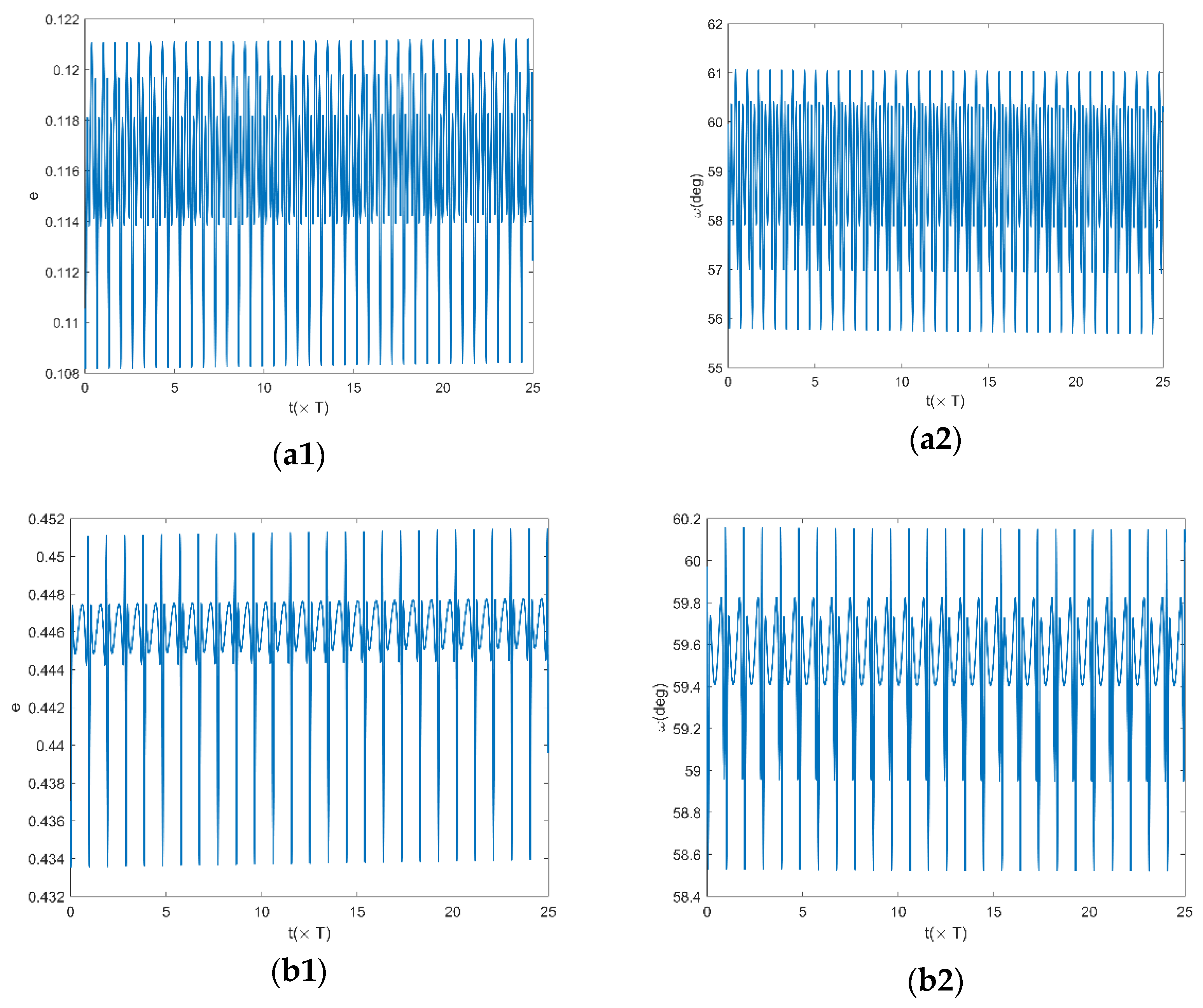
Figure 6b shows that in the case of Jupiter, critical inclinations depend on the semi-major axis and eccentricity, while for the Earth considering only the $J_2$, they are fixed (63.435 deg and 116.565 deg). The evolution of ω and $e$ for two different values of the semi-major axis and eccentricity are shown in Figure 7 and Figure 8.

Figure 7. Evolution of $\omega$ and $e$ over $25T$, (a1,a2) $a=1.6832R=120\text{,}335.334$ km, $i=63.497$ deg; (b1,b2) $a=2.1488R=153\text{,}622.009$ km, $i=63.431$ deg, where $T$ is a Jovian day.

Figure 8. $e~\omega$ evolution over $25T$, red points correspond to $a=1.6832R=120\text{,}335.334$ km and $i=63.497$ deg; green points correspond to $a=2.1488R=153\text{,}622.009$ km and $i=63.431$ deg.

For the first case in Figure 7, the amplitude of $\omega$ is about 5 deg over a time of $25T$. The amplitude of $e$ is about 0.013. For the second case, the amplitude of $\omega$ is about 1.8 deg over the same time. One can also see from Figure 8 that the amplitude of $\omega$ in the first case is much larger. This is reasonable, since the semi-major axis of the second case is larger than that of the first case.

5. Repeating Ground Track Orbits

Repeating ground track orbits are usually used for remote sensing satellites to obtain a good appearance for orbital covering. For satellites on these orbits, the ground tracks can repeat periodically. In this way, the area of Jupiter covered by the satellite can be dynamically monitored to detect the change of the target during this period of time. For example, we can make use of these orbits to detect the change of the Great Red Spot. The interval of adjacent ground track in the equator is

$$\mathsf{\Delta }\lambda =T_N\left(n_J-\dot{\mathsf{\Omega }}\right)$$

(29)

where $T_N=\frac{2\pi }{\dot{M}+\dot{\omega }}$ is the nodal period of the motion of the spacecraft. Using the mean element theory, we have [36,37]

$$\begin{array}{l}\dot{M}=n+\frac{3n{J}_2{R}^2}{2p^2}\left(1-\frac{3}{2}{\sin }^{2}i\right)\sqrt{1-e^2}+\frac{9n{J}_2^2{R}^4}{4p^4}\sqrt{1-e^2}\{\frac{1}{2}{\left(1-\frac{3}{2}{\sin }^{2}i\right)}^2\sqrt{1-e^2}\\ +\frac{5}{2}+\frac{10e^2}{3}-{\sin }^{2}i\left(\frac{19}{3}+\frac{26e^2}{3}\right)+{\sin }^{4}i\left(\frac{233}{48}+\frac{103e^2}{12}\right)\\ +\frac{e^4}{1-e^2}\left(\frac{35}{12}-\frac{35}{4}{\sin }^{2}i+\frac{315}{32}{\sin }^{4}i\right)-\frac{35J_4}{18J_2^2}{e}^2\left(\frac{9}{14}-\frac{45}{14}{\sin }^{2}i+\frac{45}{16}{\sin }^{4}i\right)\},\end{array}$$

(30)

where $n$ is the mean angular velocity. The conditions for repeating ground track orbits can be formulated as

$$D{T}_N\left(n_J-\dot{\mathsf{\Omega }}\right)=D\mathsf{\Delta }\lambda =2\pi N$$

(31)

where $D$ and $N$ are positive integers. Equation (31) implies satellites will have a repeating ground track after completing $D$ revolutions in $N$ Jovian days. The ground track repetition parameter, $Q=\frac{D}{N}$, which represents the number of orbital resolutions in a Jovian day, is widely used in engineering practice. Using this parameter combined with the definition of $T_N$, Equation (31) is equivalent to

$$Q=\frac{\dot{M}+\stackrel{.}{{\omega }_{}}}{n_J-\dot{\mathsf{\Omega }}}.$$

(32)

We can see that once $Q$ is fixed, a, e and i will be related by Equation (32). The repeating ground track orbits, which are also sun-synchronous, may play an important role in planetary exploration. For these orbits, Equation (16) was also satisfied. The change of inclinations of sun-synchronous repeating ground track orbits, with respect to the semi-major axis for different values of Q, are presented in Figure 9. One can see that for a given Q, small variations of the semi-major axis produce huge changes in the inclination. Moreover, for orbits with the same semi-major axis, the inclination,i will be larger if Q is larger. For the Earth and Mars, the inclination is not so sensitive to the semi-major axis [9].

Figure 9. Inclinations of sun-synchronous repeating ground track orbits as a function of the semi-major axis, for different values of the repetition parameter Q.

6. Conclusions

In this paper, we analyzed some special orbits around Jupiter considering only the J₂ and J₄ terms of the non-spherical gravitational potential. First, stationary orbits were investigated in spherical coordinates. The radius of stationary orbits was found to be 2.2414 Jupiter radii. The longitude drift due to the non-spherical component of the gravity field did not occur for the lack of J₂₂ terms. Moreover, a small perturbation of r and ϕ would lead to the oscillation phenomenon in the radial and North-South directions. We also showed that the perturbations of the Sun and the Galilean satellites, the main ring and the magnetic field are negligible on short time scales compared to those represented by the terms J₂ and J₄. However, the obtained solutions may be incorrect on long time scales. Then, sun-synchronous orbits, orbits at critical inclinations, and repeating ground track orbits were discussed based on the mean-element theory. The results showed that only one meaningful inclination exists for sun-synchronous orbits when a and e are fixed in a suitable range. Additionally, only two critical inclinations exist for the critical orbits. Repeating ground track orbits, which are also sun-synchronous, were also calculated here. The traditional frozen orbits were not discussed because the J₃ term was not taken into account in our gravity model. However, we remark that there may exist some non-traditional frozen orbits around Jupiter, which will be left for our future investigations.

The dynamics around Jupiter are very complicated and even if some perturbations can be neglected for preliminary orbit design, other effects should be considered. For example, orbits at low-to-moderate inclinations within a few Jovian radii may loiter inside Jupiter’s radiation belts. This can lead to considerable risk for the integrity of a satellite. However, we believe that our work can help to reduce or eliminate the need for station keeping in future space mission around Jupiter.