Large-Eddy Simulation of Low-Pressure Turbine Cascade with Unsteady Wakes

Abstract

To better understand the wake effects at low Reynolds numbers, large-eddy simulations of a 50% reaction low-pressure turbine stage and a linear cascade with two different bar wake generators were carried out for a chord Reynolds number of 50,000. For the chosen front-loaded high-lift airfoil, the endwall structures are stronger than for more traditional mid-loaded moderate-lift airfoils. By comparing the 50% reaction stage results with the bar wake generator results, insight is gained into the effect of the three-dimensional wake components on the downstream flow field.For the cases with bar wake generator, the endwall boundary layer is growing faster because of the relative motion of the endwall with respect to the freestream. The half-width of the wake is approximately matched for the larger one of the two considered bar wake generators. To improve the quality of the phase-averaged flow fields, the proper orthogonal decomposition was employed as a filter to remove the low-energy unsteady flow field content. Both the mean flow and filtered phase-averaged flow fields were analyzed in detail. Visualizations of the phase-averaged flow field reveal a periodic suppression of the laminar suction side separation from the downstream airfoil even for the smaller bar wake generator. The passage vortex is entirely suppressed for the 50% reaction stage and for the larger bar wake generator. Furthermore, the phase-averaged data for the 50% reaction stage reveal a new longitudinal flow structure that is traced back to near-wall wake vorticity. This flow structure is missing for the bar wake generator cases.

1. Introduction

In modern high-bypass jet engines, the low-pressure turbine (LPT) is driving the fan which produces most of the thrust. Due to the high fan power requirements and the limitation on the LPT stage pressure ratio, the LPT is a large and heavy component. This has motivated research to reduce the weight and improve the overall efficiency of the LPT. Researchers at the Air Force Research Laboratory (AFRL) developed the front-loaded high-lift L2F research LPT blade specifically for investigating the aerodynamics of highly loaded profiles [1]. A higher loading would allow for a lower overall blade count and thus a reduced LPT weight. This, however, comes at the cost of considerably increased endwall losses when compared to mid or aft-loaded profiles [2,3,4].

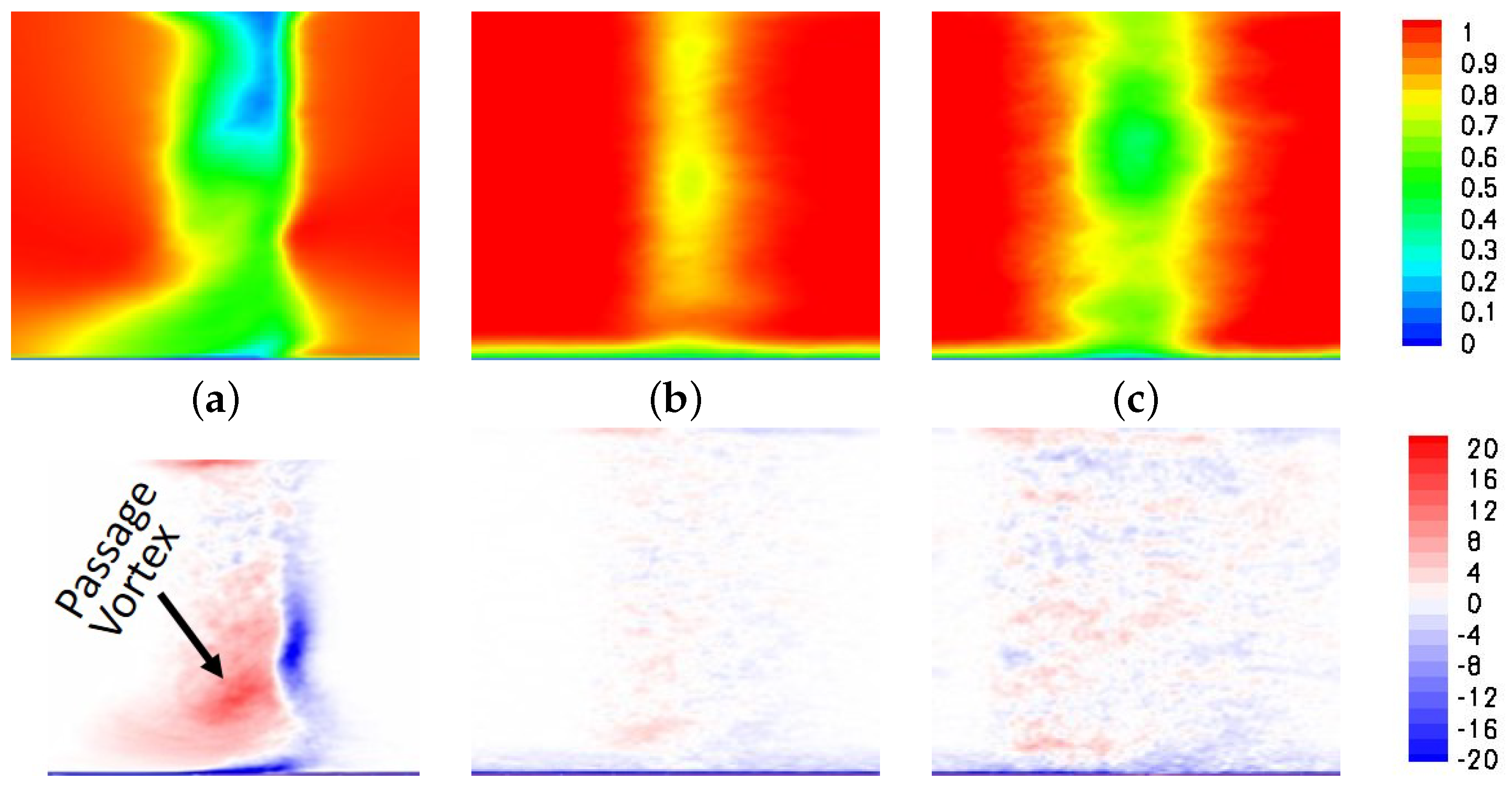
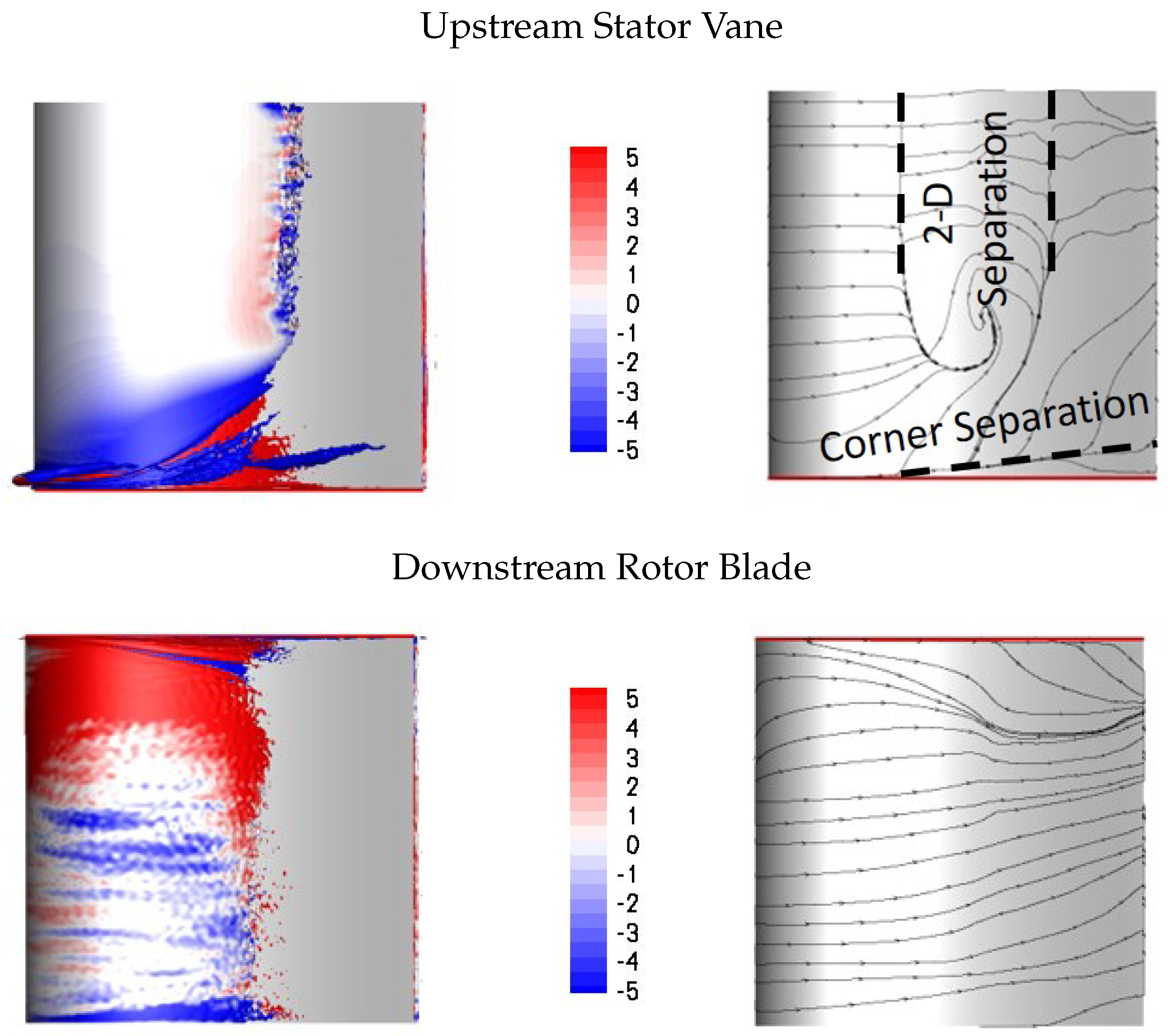
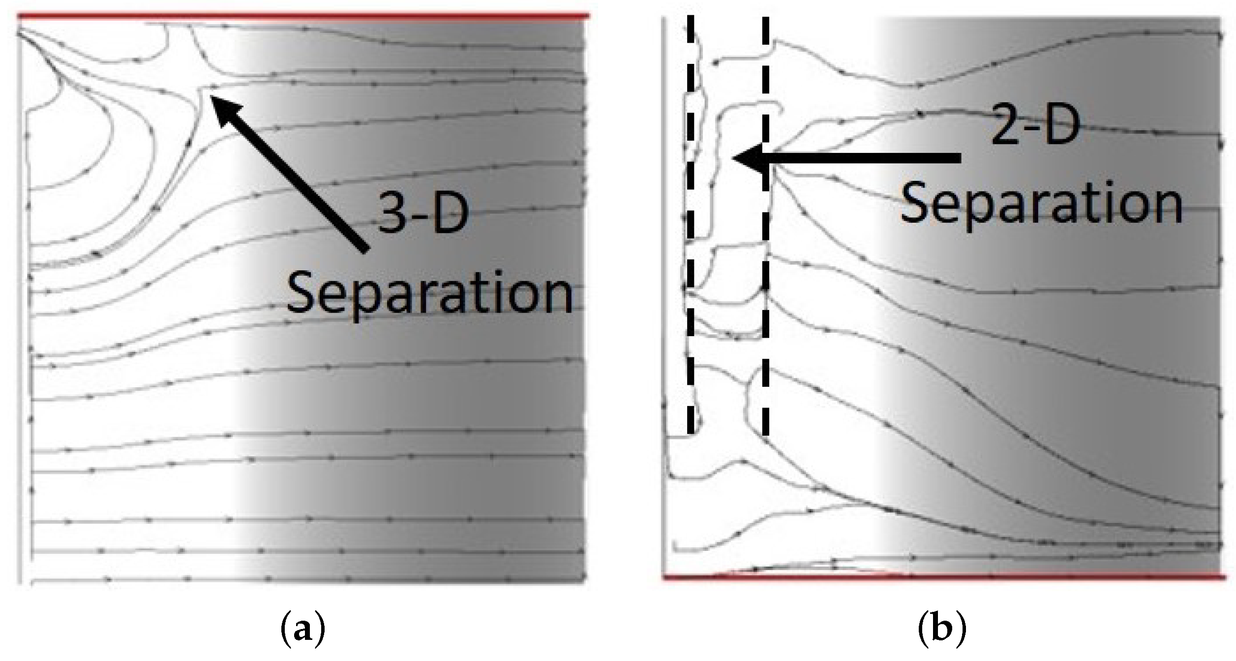
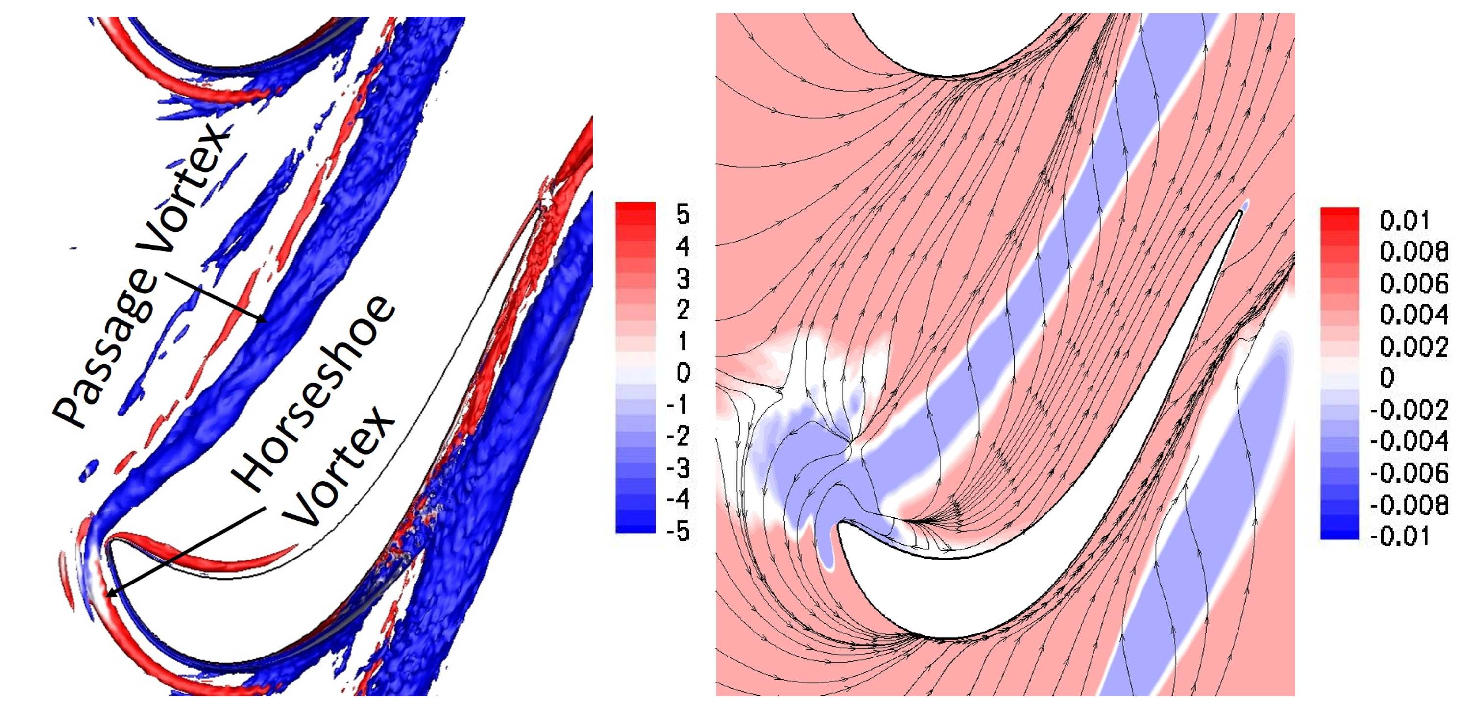
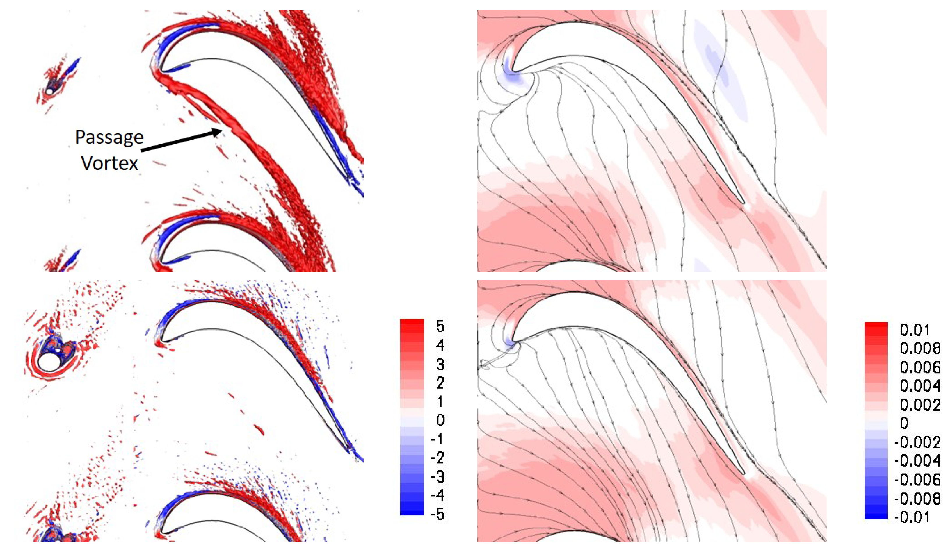
More recently, researchers discovered that the suction side corner separation and passage vortex (PV) are major contributors to the endwall losses. The PV stems from the pressure side leg of the horseshoe vortex (HV) that is a product of the interaction of the turbulent boundary layer with the leading edge of the blade [5,6]. The secondary flow, which results from an imbalance of the radial centrifugal acceleration and pressure gradient near the endwall, feeds and strengthens the PV and weakens and dissipates the suction side leg of the HV. Langsten et al. [7,8] and Sieverding [9] provided review papers on the endwall structures. Visualizations and descriptions of the full three-dimensional (3-D) flow field topology were provided by Wang et al. [10], Sieverding [9], Goldstein and Spores [11], Sharma and Butler [12], and Kang and Hirsch [13], among others. The effect of the endwall boundary layer thickness on the total pressure losses was investigated by Hodson and Dominy [14]. They found that as the endwall boundary layer thickness increases, the PV moves farther away from the suction surface and the total pressure losses increase near the endwall but remain unchanged near mid-span.

Turbulent junction flows, such as seen at the junction of the blade leading edge and the endwall, exhibit a bimodal behavior that is characterized by a more or less random switching between a zero-flow state with weak HV and a back-flow state with strong HV that is located closer to the leading edge [15]. Smoke line visualizations by Wang et al. [10] for a linear turbine cascade at a Reynolds number of 10,000 clearly displayed a bimodal behavior of the HV with a dimensionless frequency of $f{C}_{ax}/v_{in}=0.6$ where $C_{ax}$ is the axial chord and $v_{in}$ is the inlet velocity. Large-eddy simulations (LES) by Robison et al. [16] of a canonical junction flow indicated a correlation of the bimodal behavior with upstream turbulent boundary layer events. Simulations by Gross et al. [17,18] and measurements by Veley et al. [19,20] and Babcock et al. [21] for a L2F cascade revealed an intermittent loss of coherence of the PV that appeared related to the bimodal behavior. Since the PV is a large contributor to the losses, this suggests that the bimodal behavior of the HV has an impact on the overall efficiency of the LPT. Because the energy in the PV is lost, efforts are being made to develop active flow control strategies to diminish the coherence of the PV. For example, pulsed endwall jets near the leading edge of the blade were found to be moderately successful and allow for a reduction of the overall passage total pressure losses by several percentage points [21,22].

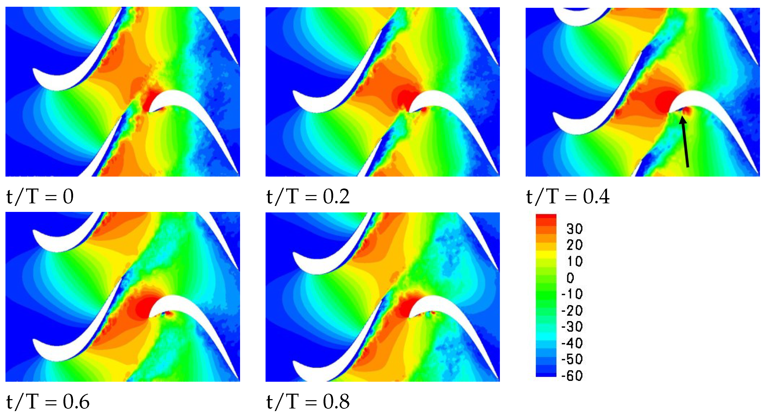
The LPT is typically comprised of more than one stage. Each LPT stage consists of stator vanes and rotor blades. The periodic passing of the rotor blades with respect to the stator vanes results in an unsteady flow field that is characterized by elevated freestream turbulence and wakes that periodically impinge on the leading edge and suction surface of the downstream airfoils. As a result, the flow through an LPT cascade with passing wakes is different from the flow through an isolated linear cascade without upstream wakes. Meyer [23] stated that wakes cause a periodic perturbation in the freestream in the form of a momentum deficit or “negative jet”. While the wake effect on the suction side boundary layer separation and associated losses has been investigated in considerable detail, the effect on the endwall flow structures and losses is less well understood. Wind tunnel experiments with unsteady wakes pose many challenges. Annular cascades more closely represent the unsteady flow in turbine engines. Such systems, however, are complicated, expensive and difficult to instrument [24]. In linear cascade experiments, two-dimensional (2-D) wakes without pronounced secondary flow can be generated with moving-bar wake generators. Although bar wake generators provide an accurate representation for the 2-D wake component, they cannot accurately represent the endwall flow structures of front-loaded high-lift airfoils. Recently developed new devices for investigating unsteady wake effects in linear cascades, such as the periodic unsteadiness device proposed by Fletcher et al. [25,26], cut down even more on the mechanical complexity and allow for a precise adjustment of the wake velocity deficit and frequency.

The vast majority of the earlier wake-effect research is for aft-loaded airfoils such as the T106 and the Pratt and Whitney Pack B. Compared to the L2F, for aft-loaded airfoils the laminar separation from the suction surface is more severe and the endwall losses are smaller. Experiments by Schulte and Hodson [27,28] and Kaszeta et al. [29] revealed that the passing wakes cause bypass-transition of the suction side boundary layer. Direct numerical simulations (DNS) and LES of a T106 cascade with periodic passing wakes by Wu and Durbin [30] and Michelassi et al. [31,32] showed that the wakes align with the principal axis of the main flow and the resulting stretching generates streamwise vortices. Stieger and Hodson performed Laser Doppler Velocimetry measurements in a linear cascade with passing wakes [33,34]. They reported that the flow was accelerated upstream and decelerated downstream of the wake impingement point. This was found to destabilize the flow and accelerate the roll-up of the separated boundary layer into spanwise vortices. It was also shown that the wakes are accelerated and stretched as they pass through the passage and that the turbulent kinetic energy of the wake increases outside of the boundary layer. In AFRL experiments with moving bar wake generator by Nessler et al. [35,36] for a Reynolds number of 25,000, laminar separation from the suction surface was almost completely suppressed. Experiments by Volino [37] revealed a complete suppression of laminar separation for high wake passing frequencies and an intermittent suppression of flow separation for low wake passing frequencies. Experiments by Schmitz et al. [24] considered a single stage rotating rig with transonic LPT blades. Observed inconsistencies of the endwall data led to the conclusion that a need exists for models that accurately capture the secondary flow effects and the endwall losses. Experiments in an annular cascade with bar wake generator by Sinkwitz et al. [38] revealed that the wakes weakened the PV and the shed vortex. Cui et al. [39,40] employed LES for investigating the effect of the endwall boundary layer state (laminar or turbulent) and upstream wakes (with secondary flow structures). With turbulent endwall boundary layer and passing wakes, the total pressure losses were increased substantially over a reference case with laminar endwall boundary layer and no wakes. More recently, Romero and Gross [41] and Robison and Gross [42] performed LES of a linear 50% reaction turbine stage with L2F blades. The passing wakes were shown to greatly diminish the coherence of the HV and PV and suppress laminar boundary layer separation from the suction surface. A new transient longitudinal flow structure was observed near the pressure side trailing edge.

In summary, front-loaded high-lift LPT airfoils were found to suffer from increased endwall losses. Prior research aimed at a better understanding of the source of the increased endwall losses has neglected the wake effect. Most of the earlier wake effect research is for aft-loaded airfoils that do not suffer from large endwall losses. The primary focus of the earlier wake effect research was on the suppression of laminar separation from the suction surface and not on the wake effect on the endwall flow. The majority of the experimental wake effect research employed bar wake generators that do not model the strong endwall structures downstream of front-loaded high-lift airfoils.

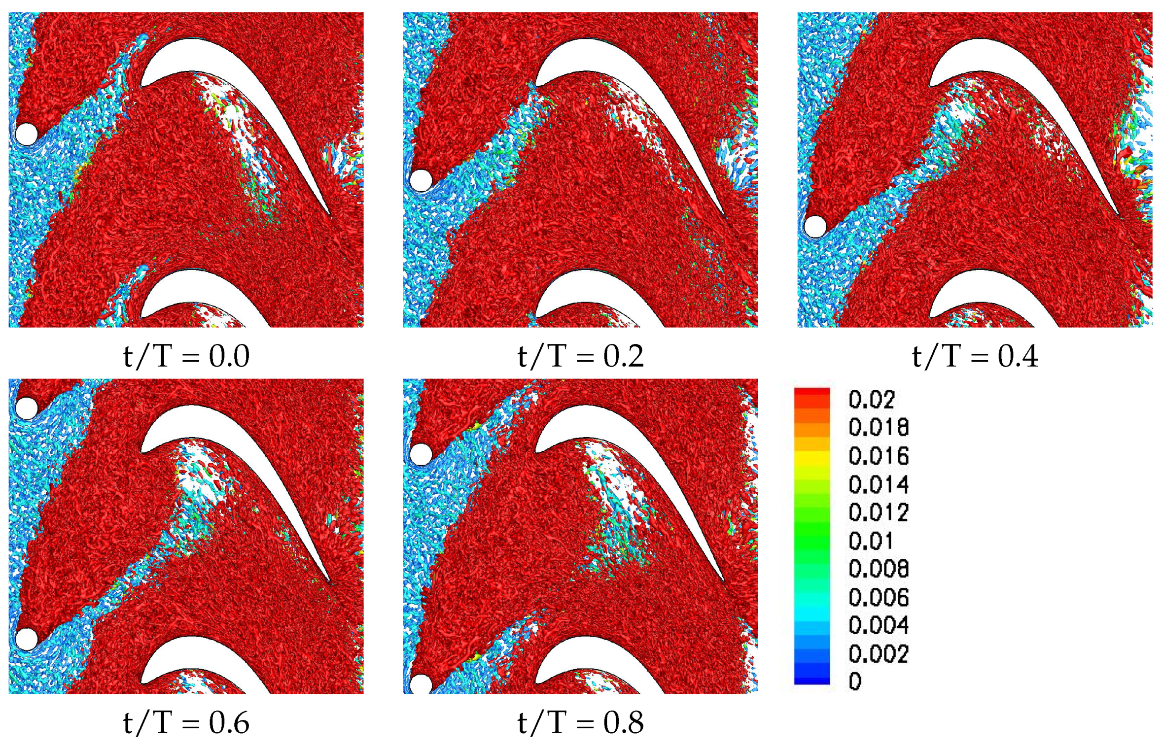
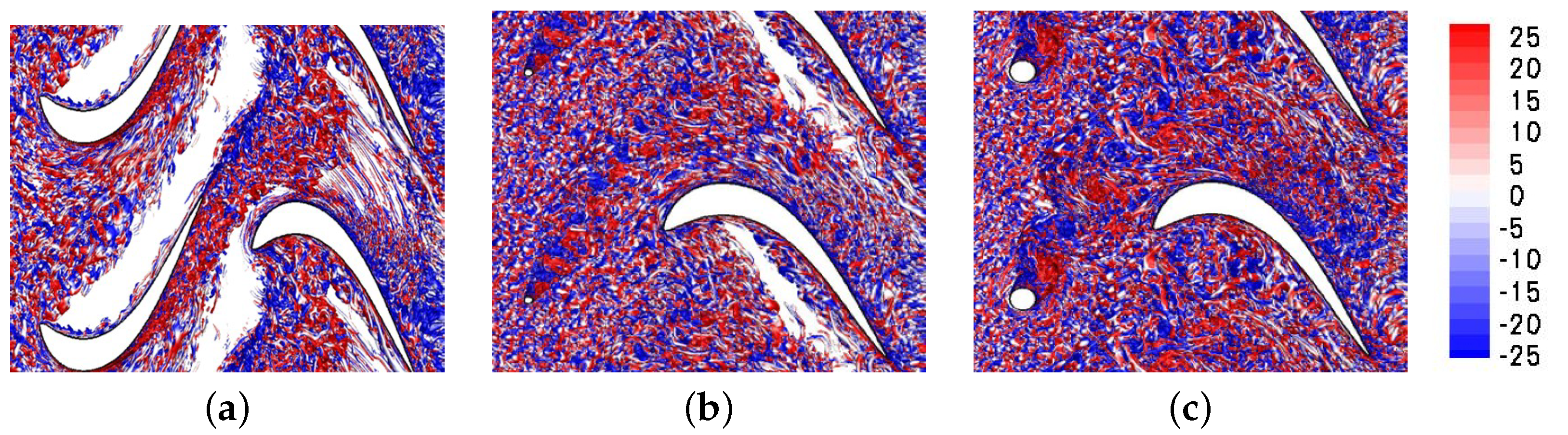
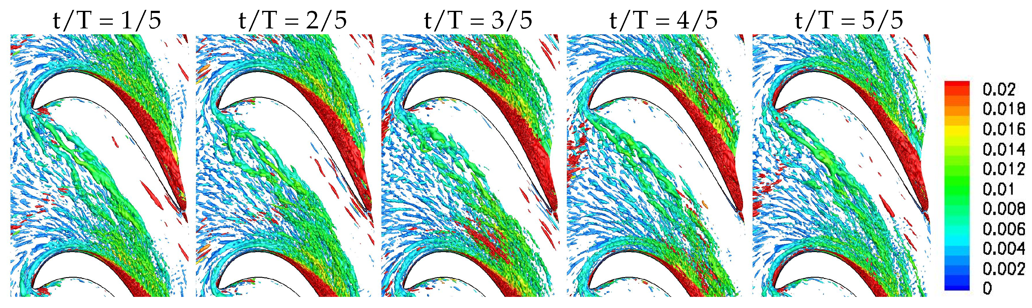
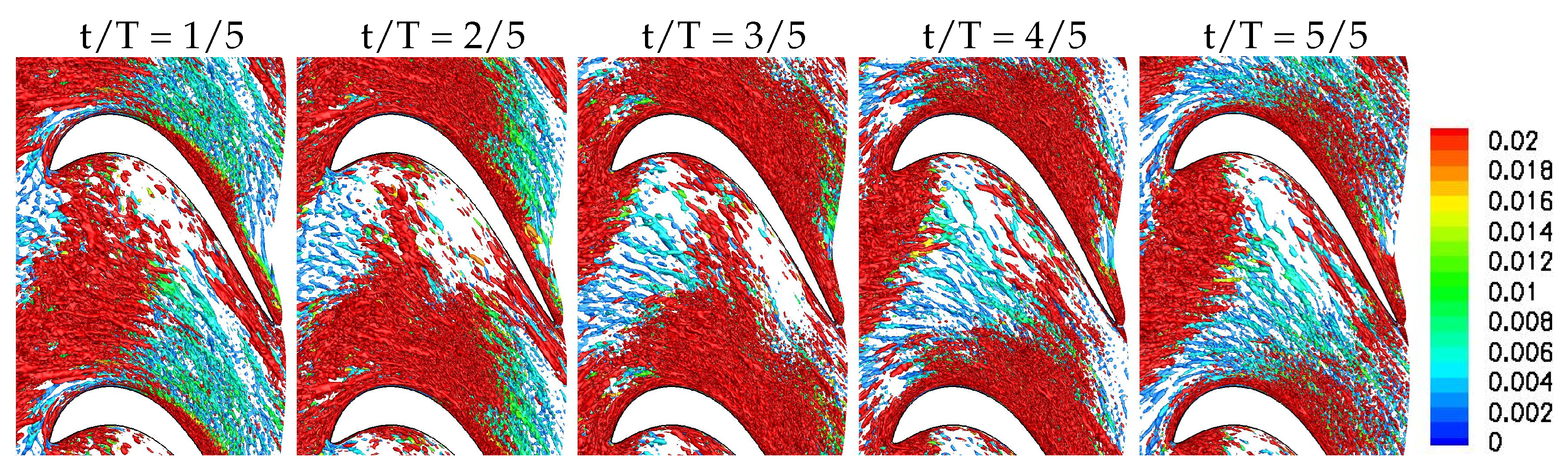
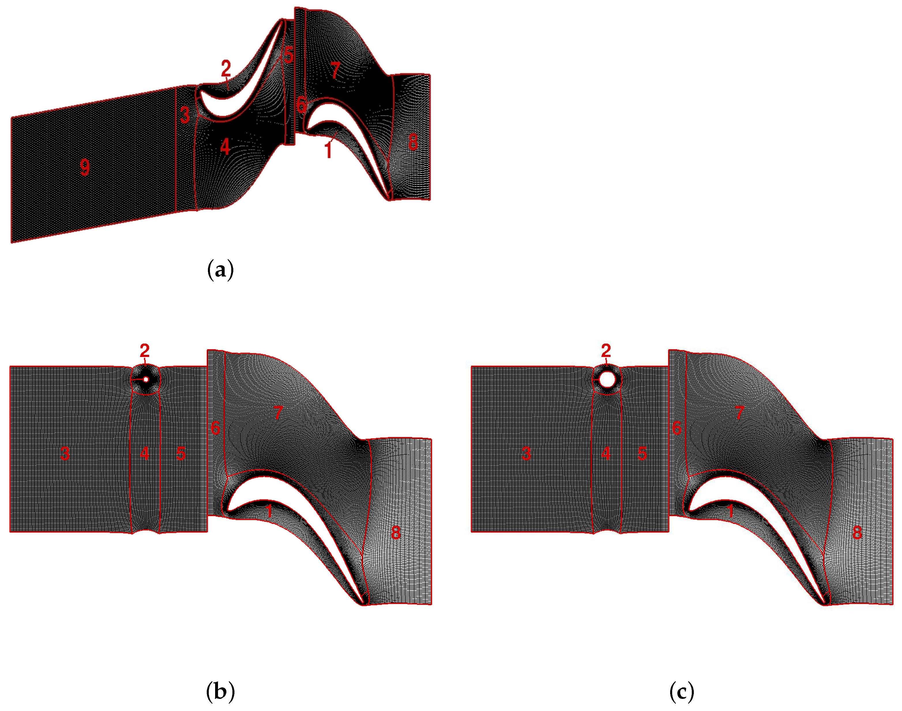
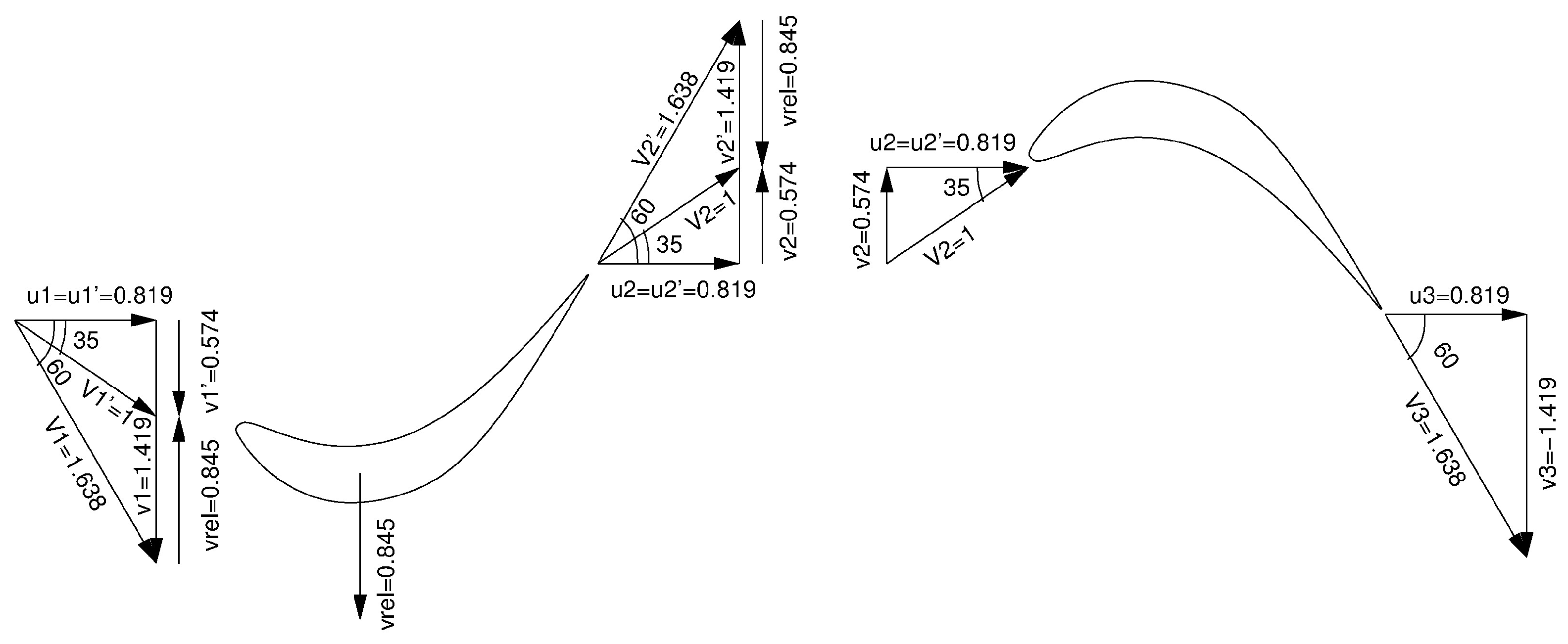
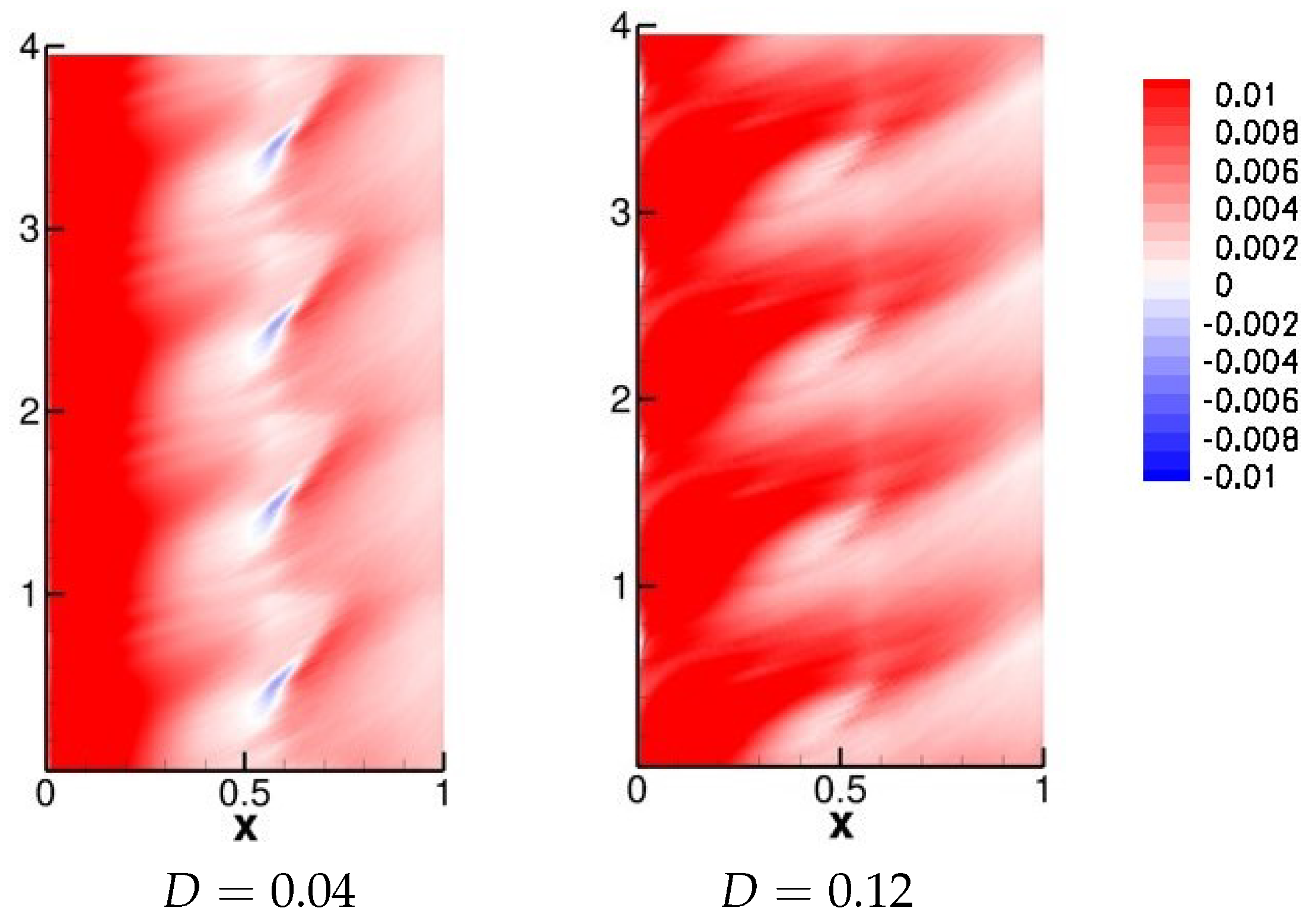
These research needs motivated the present LES for a front-loaded high-lift airfoil at a chord Reynolds number of 50,000. For the chosen Reynolds number, the laminar separation is substantial, thus allowing for a clear identification of the wake effect. Three simulations are presented. The first simulation is for a full 50% reaction stage with identical stator and rotor airfoils. For the other two simulations, the upstream L2F blade was replaced by moving circular cylinder bar wake generators with a diameter of 0.04 and 0.12 axial chord. The bar wake generators create 2-D wakes without significant secondary flow structures near the endwall. The present simulations provide novel insight into the wake effect on the endwall flow for front-loaded high-lift LPT airfoils at the low end of the Reynolds number range. By comparing the results with LPT airfoil (50% reaction stage) and bar wake generator, the contribution of the 3-D near-wall wake components is revealed. For the discussion of the unsteady flow physics, the flow fields are visualized in unprecedented detail. The results obtained from the three simulations are presented side by side and compared with respect to the mean flow topology and the phase-averaged unsteady flow fields.

2. Methodology

2.1. Numerical Method

The compressible Navier–Stokes equations in the finite-volume formulation were solved with a research computational fluid dynamics code by Gross and Fasel [43,44]. The convective terms were discretized with a ninth-order-accurate weighted essentially non-oscillatory scheme. A fourth-order-accurate discretization was employed for the viscous terms and the time derivatives were computed with the second-order-accurate implicit trapezoidal rule. Since no explicit subgrid stress model was employed for the present simulations, they are here referred to as implicit large-eddy simulations (ILES). For ILES, the numerical scheme removes the proper amount of energy at the smallest grid scales. The dynamic viscosity, $\mu$, was obtained from Sutherland’s law.

2.2. Sliding Mesh

The sliding mesh technique proposed in Romero and Gross [45] is based on the assumption that both grid and data are periodic in the pitchwise direction at the interface where the relative motion occurs. This situation is characteristic of turbomachinery stages where stator vanes and rotor blades are spaced at a constant pitch (azimuthal interval). Close to the interface, the grid is assumed to be perfectly equidistant and rectangular such that the flow field in the pitchwise direction can be expressed as a function of the pitchwise cell index, i. The total number of cells at the interface in the pitchwise direction, counted from 0, is $ix$. The shift is accomplished using Fourier transforms (which are by nature periodic). The forward Fourier transforms are

$$\begin{array}{ccc}\hfill {\widehat{u}}_{c,j}& =& \sum _{i=0}^{ix}{u}_{i}cos\frac{2\pi ij}{ix+1}\hfill \end{array}$$

(1)

$$\begin{array}{ccc}\hfill {\widehat{u}}_{s,j}& =& \sum _{i=0}^{ix}-u_{i}sin\frac{2\pi ij}{ix+1},\hfill \end{array}$$

(2)

where $1<j<(ix+1)/2$ is the Fourier mode number. Fourier mode $j=0$ is computed from,

$${\widehat{u}}_{c,0}=\sum _{i=0}^{ix}{u}_i.$$

(3)

The backward transformation is

$$u_i=\frac{1}{ix+1}\left\{{\widehat{u}}_{c,0}+2\sum _{j=1}^{(jx+1)/2}\left[{\widehat{u}}_{c,j}cos\frac{2\pi (i+s)j}{ix+1}-{\widehat{u}}_{s,j}sin\frac{2\pi (i+s)j}{ix+1}\right]\right\},$$

(4)

where $s=v_{rel}t/S\times ix$ is the relative pitchwise shift along the interface, $v_{rel}$ is the velocity of the relative motion, S is the blade pitch, and t is time.

2.3. Synthetic Eddy Method

The divergence-free isotropic synthetic eddy model (SEM, Jarrin et al. [46], Poletto et al. [47]) was employed for initiating (or seeding) the turbulent endwall boundary layer. Because this model is driven by a random number generator, it does not favor certain frequencies (or wavelengths). Mankbadi et al. [48] compared the SEM with digital filtering (Klein et al. [49]) and found that both models require an adjustment length of six boundary layer thicknesses.

A box with volume $V_b$ is initialized with a random distribution of $N=5000$ eddies. The box has the dimensions of the inflow boundary layer thickness, $\delta$, and pitch, and a streamwise extent of

$$2{\sigma }_{max}=2\underset{N}{max}\left({\sigma }_k\right).$$

(5)

The size of each eddy, k,

$${\sigma }_k=max(min[\ell ,0.41\delta ],{\Delta }_{max})$$

(6)

is defined based on the turbulent length scale at the wall-normal location of the eddy,

$$\ell =\frac{k^{\frac{3}{2}}}{,}\prime$$

(7)

with turbulence kinetic energy (TKE), k, and dissipation rate, $\epsilon$. The grid length scale,

$${\Delta }_{max}=max(\Delta x,\Delta y,\Delta z),$$

(8)

is taken as the maximum of the cell dimensions, $\Delta x$, $\Delta y$, and $\Delta z$, at the location of the eddies. Boundary layer profiles obtained from a precursor Reynolds-averaged Navier–Stokes (RANS) calculations with k-$\omega$ model (Figure 1) served as basis for the SEM and provided the mean quantities, $\overline{\mathbf{u}}\left(y\right)$, $k\left(y\right)$, $\epsilon \left(y\right)$, and $\delta$, where y is the wall distance.

In the ILES, the eddies induce velocities at the inflow boundary of the computational domain. The velocity fluctuations are computed as the sum over all N eddies,

$${\mathbf{v}}^{\prime }=\sqrt{\frac{1}{N}}\sum _N\frac{{\mathbf{r}}_k\times {\mathbf{e}}_k}{{\mathbf{r}}_k^3}f({\sigma }_k,{\mathbf{r}}_k)\times \sqrt{\frac{2}{3}k},$$

(9)

and added to the mean flow profile, $\overline{\mathbf{u}}\left(y\right)$. Here,

$${\mathbf{r}}_k=\frac{\mathbf{x}-{\mathbf{x}}_k}{{\sigma }_k}$$

(10)

is the location vector from an eddy to a point on the inflow boundary normalized by the eddy size. The TKE, k, is taken at the wall-normal location of the individual eddies. The orientation vectors for each eddy, k, are randomized with either plus or minus one,

$${\mathbf{e}}_k=\left[\begin{array}{c}random(\pm 1)\\ random(\pm 1)\\ random(\pm 1)\end{array}\right].$$

(11)

The shape function is given by

$$f({\sigma }_k,{\mathbf{r}}_k)=\left\{\begin{array}{cc}\sqrt{\frac{16V_b}{15\pi {\sigma }_k^3}}{sin}^2\left(\pi \right|{\mathbf{r}}_k\left|\right)|{\mathbf{r}}_k|\hfill & |{\mathbf{r}}_k|<1\hfill \\ 0\hfill & otherwise\hfill \end{array}\right.$$

(12)

The pressure and temperature are obtained from the approach flow stagnation values assuming an isentropic state change. After each timestep, the vortices are convected in the streamwise direction by the freestream velocity. Vortices that leave the box are regenerated at random locations and with random orientations on the inflow plane of the box.

2.4. Non-Dimensionalization

All quantities were made dimensionless with the axial chord length, $C_{ax}$, and the inlet velocity, density, temperature, and dynamic viscosity. The Reynolds number based on relative inlet velocity and axial chord length for the vane and blade was 50,000. The reference Mach number for the simulation was $M_{ref}=0.1$ and low enough to satisfy the incompressible flow assumption. Based on the isentropic flow relationships, for a Mach number of 0.1, the stagnation density is 0.5% above the freestream density. Compared to the changes in the other flow quantities, for the chosen reference Mach number the changes in density are insignificant. The Prandtl number was $Pr=0.72$ and the inlet temperature was 300 K.

2.5. Computational Grid

Three computational grids were generated. The first grid is for a 50% reaction stage with two L2F airfoils with an axial separation (stator trailing edge to rotor leading edge) of $0.3$. The second and third grids are for an L2F airfoil with upstream cylinder bar wake generator. The cylinders have diameters of $D=0.04$ and $0.12$ and the axial distance of the cylinder center to the leading edge of the blade is 0.6. The Reynolds number based on cylinder diameter is 2000 for $D=0.04$ and 6000 for $D=0.12$. A Poisson grid generator [50] was employed to generate two-dimensional (2-D) grids with nine and eight blocks (Figure 2 and

Table 1. Block grid resolutions.

Block	Number of Cells
	50% Reaction	Bar Wake Generator
	Stage	$\mathit{D}=0.04$	$\mathit{D}=0.12$
1	512 × 48	512 × 48	512 × 48
2	512 × 48	138 × 96	138 × 96
3	34 × 176	159 × 176	159 × 176
4	208 × 128	41 × 148	41 × 148
5	18 × 176	60 × 176	60 × 176
6	18 × 176	18 × 176	18 × 176
7	208 × 128	208 × 128	208 × 128
8	24 × 176	24 × 176	24 × 176
9	283 × 176	-	-

). The x-coordinate points in the axial direction and the y-coordinate points in the pitchwise direction. The z-coordinate is normal to the endwall. Grid line stretching was used at the block 8 outflow boundary to dissipate flow structures. Cells were clustered near the stator vane, rotor blade, and cylinder to resolve the boundary layers. Near the sliding mesh interface, the grids were modified to be perfectly equidistant in the axial and pitchwise direction. Blocks 9 and 3 were added at the inflow boundary for accommodating the approach endwall boundary layer. For the 50% reaction stage grid, block 9 is equidistant in the axial and pitchwise direction and has an axial extent of roughly two axial chord lengths. Block 3 for the simulation with bar wake generator has an axial extent of only $0.9$ as the endwall boundary layer was found to grow faster than for the 50% reaction stage.

The two-dimensional (2-D) grids were extruded over a distance of one axial chord length in the spanwise direction. Towards that end, a grid line distribution that provides grid line clustering near the endwall to resolve the endwall flow structures and boundary layer was employed. The grid line distribution blends towards an equidistant spacing away from the wall,

$$\begin{array}{lll}{z}_0\hfill & =& 0\hfill \end{array}$$

(13)

$$\begin{array}{lll}{z}_1\hfill & =& \Delta z\hfill \end{array}$$

(14)

$$\begin{array}{lll}{z}_k\hfill & =& z_{k-1}+\left[0.1{\left(\frac{k-kx}{2-kx}\right)}^c+1\right](z_{k-1}-z_{k-2})\mathrm{for} k\ge 2.\hfill \end{array}$$

(15)

Here, k is the spanwise grid line index and $kx=256$ is the number of grid lines in the spanwise direction. The wall-normal grid line spacing at the endwall is $\Delta z={10}^{-4}$. The total number of cells is 43,200,512 for the 50% reaction stage and 22,996,560 for the bar wake generator cases.

The near-wall grid resolution in wall units for the approach boundary layer is $\Delta x^{+}\approx 16$, $\Delta y^{+}\approx 16$, and $\Delta z^{+}\approx 0.1$ upstream of the stator and $\Delta x^{+}\approx 16$, $\Delta y^{+}\approx 20$, and $\Delta z^{+}\approx 0.15$ upstream of the bar wake generators and thus close to those employed by Nicoud and Ducros [51] for their LES test problem (28, 8.8, and 2.1, respectively). Contours of the near-wall grid line spacing in wall units for the endwall of blocks 1 and 7 are provided in Figure 3. Above the blade, the streamwise, pitchwise, and wall-normal grid line spacing in wall units are roughly 25, 25, and 0.3 which is acceptable for wall-resolved LES. The present grid resolution in wall units is comparable to that of an earlier LES of a linear LPT cascade for a Reynolds number of $\mathrm{100,000}$ [18]. For this earlier LES, a detailed validation with wind tunnel data was carried out in lieu of a grid convergence study. The good agreement of these earlier LES results with the experimental data supports the choice of the grid resolution for the present simulations.

The number of cells in the boundary layer ($z\le \delta$) and viscous sublayer ($z^{+}\le 10$) for the approach boundary layer of the 50% reaction stage simulation (block 9) is plotted in Figure 4. Because the wall-normal grid line distribution is constant, as the boundary layer grows in the streamwise direction, the number of cells across the boundary layer is increasing. At the passage inflow, the number of cells across the laminar sublayer is ≈20 and the number of cells across the boundary layer is ≈90, which is sufficient for LES of LPT flows [52].

2.6. Boundary Conditions

All walls were considered as adiabatic. Flow periodicity was enforced in the pitchwise direction. Non-reflecting boundary conditions [53] were applied at the inflow and outflow boundaries. Symmetry conditions (slip wall) were enforced at the open spanwise boundary.

2.7. Case Description

The L2F airfoil was chosen for both the rotor blade and the stator vane. The L2F design inlet and outlet angle are ${\alpha }_{in}=35deg$ and ${\alpha }_{out}=-60deg$, respectively, and the blade pitch is $S=1.221$. Since the Reynolds number was computed with the inlet velocity, in the simulation, the rotor blade inflow velocity was set to $V_2=1$. Based on mass conservation, an estimate for the rotor exit velocity can be obtained,

$$V_3=\frac{cos35deg}{cos60deg}{V}_2=1.63830.$$

(16)

The axial and pitchwise components of the rotor blade inlet velocity are $u_2=V_{2}cos35deg=cos35deg$ and $v_2=V_{2}sin35deg=sin35deg$. The axial velocity at the vane outlet, $u_2^{\prime }$, has to match the axial velocity at the rotor inlet $u_2^{\prime }=u_2$. Dashes are here used to indicate velocity components in the moving reference frame of the vane (relative motion: in actual turbines, the blades are moving and the vanes are stationary; in the simulation the vanes are moving and the blades are stationary). For a relative vane inlet velocity of $V_1^{\prime }=1$, the relative vane outlet velocity becomes

$$V_2^{\prime }=\frac{cos35deg}{cos60deg}{V}_1^{\prime }.$$

(17)

The pitchwise velocities in the stationary frame have to match at the vane–blade interface,

$$V_2^{\prime }sin60deg-v_{rel}=sin35deg.$$

(18)

From this, the relative velocity of the vane is obtained,

$$v_{rel}=cos35degtan60deg-sin35deg=0.845237.$$

(19)

The time taken for the vane to travel one pitch length (wake passing period) is

$$T=\frac{S}{v_{rel}}=1.44457.$$

(20)

The vane inlet axial velocity is the same in the stationary and moving frame, $u_1=u_1^{\prime }=cos35deg$. The pitchwise velocity in the stationary frame is

$$v_1=v_1^{\prime }-v_{rel}=-sin35deg-v_{rel}=-cos35degtan60deg.$$

(21)

The vane inlet velocity magnitude in the stationary frame then becomes

$$V_1=\sqrt{u_1^2+v_1^2}=\frac{cos35deg}{cos60deg}=1.63830,$$

(22)

and the vane inlet flow angle in the stationary frame is

$${\alpha }_1={tan}^{-1}\frac{v_1}{u_1}=-60deg.$$

(23)

For the bar wake generator simulations, the velocity magnitude and direction at the block 6 inflow boundary are $V_2=1$ and ${\alpha }_{in}=35deg$. The inflow velocities are $u_2=0.819$ and $v_2=0.574$. The cylinders have the same relative pitchwise velocity as the rotor blade. Because blocks 2–5 move with the cylinder, for the bar wake generator simulations the endwall moves relative to the fresstream. This results in a cross-flow velocity component near the endwall that leads to a faster growth of the endwall boundary layer compared to the 50% reaction stage simulation. Figure 5 summarizes the velocities for the 50% reaction stage.

The computational time step for all simulations was $\Delta t=0.00481522$ (300 timesteps per wake passing period). The number of periods for the phase averaging and the time intervals for the time averaging are provided in

Table 2. Number of periods for phase averaging and time interval for time averaging.

	Number of Periods	Time Interval
L2F	8	11.56
Small Cylinder, D = 0.04	9	13.01
Large Cylinder, D = 0.12	7	10.11

.

2.8. Proper Orthogonal Decomposition

The proper orthogonal decomposition (POD) [54] decomposes a time-dependent velocity field into a sum of products of time-coefficients, $a_i\left(t\right)$, and modes, ${\mathbf{q}}_i\left(\mathbf{x}\right)$,

$$\mathbf{v}(\mathbf{x},t)=\sum _i{a}_i\left(t\right){\mathbf{q}}_i\left(\mathbf{x}\right).$$

(24)

The magnitudes of the associated eigenvalues, ${\lambda }_i$, are identical to two times the kinetic energy content of the respective modes. The POD modes form an orthogonal basis and are here sorted according to their energy content. The present POD results were obtained with the “snapshot” method by Sirovich [55].

3. Results

3.1. Approach Flow Analysis

Iso-surfaces of the Q-criterion by Hunt [56] flooded by the streamwise velocity for the approach flow endwall boundary layer are provided in Figure 6. For all cases, the boundary layer grows in the streamwise direction and is fully turbulent when it reaches the stator vane or cylinder leading edge. Near-wall streaky structures, likely resulting from cross-flow instability, can be observed for the bar wake generator cases (e.g., red circle in Figure 6).

Velocity profiles $1/2C_x$ upstream of the stator vane and bar wake generator leading edge are provided in Figure 7. The subscripts 35 and 60 refer to velocity components relative to the 35 and 60 deg incidence angle. For the 50% reaction stage case, $v_{35}$ is zero and $u_{35}$ is almost 1 in the freestream. For the bar wake generator cases, because the endwall is moving relative to the freestream, $u_{35}$ and $v_{35}$ are non-zero at the endwall which is typical for actual turbines. The $v_{60}^{\prime }$ component has a small non-zero region just above the endwall and $u_{60}^{\prime }$ approaches $1.6$ in the freestream.

3.2. Wake Analysis

Iso-surfaces of the Q vortex identification criterion flooded by the wall-normal distance for the phase-averaged flow fields are displayed in Figure 8, Figure 9 and Figure 10. Since the iso-surfaces are flooded by the distance to the endwall, near-wall structures can be differentiated from flow features farther away from the endwall. The upstream L2F and the bar wake generators shed unsteady wakes as they travel in the pitchwise (transverse) direction. The iso-surfaces suggest that the wake width for the upstream L2F and smaller bar wake generator is similar shortly upstream of the downstream rotor blades. As the wakes pass through the downstream passage they stretch to form a $\mathsf{\Lambda }$ shape. This can be explained by the faster flow in the center of the passage compared to the slower flow near the blades. The wake appears much wider for the larger diameter case. For the 50% reaction stage simulation, a transient longitudinal flow structure appears intermittently near the trailing edge of the pressure side.

Instantaneous iso-surfaces of Q flooded by the wall-normal vorticity, ${\omega }_z$, are presented in Figure 11. The bar wake generator cases exhibit a von Kármán vortex street. For the smaller diameter cylinder, the vortices are spaced more closely. No distinct spanwise coherent structures are visible for the 50% reaction stage simulation.

The streamwise velocity and streamwise vorticity at the stator inflow plane were computed from the time-averaged flow field as $u_{in}=ucos\left(35deg\right)+vsin\left(35deg\right)$ and ${\omega }_{in}={\omega }_{x}cos\left(35deg\right)+{\omega }_{y}sin\left(35deg\right)$, respectively. Iso-contours of both quantities for the upstream face of block 6 ($x=-0.149$) are provided in Figure 12. These visualizations allow for a comparison of the wake shape and velocity deficit. The wake for the upstream L2F has a considerably larger velocity deficit than the wake for the small-diameter cylinder. The wake for the former is also wider. For the large-diameter cylinder, the wake width is about the same as for the 50% reaction stage but the velocity deficit is smaller. As a result of the moving wall, the endwall boundary layer for the bar wake generator cases is thicker, as explained earlier. The ${\omega }_{in}$ contours reveal strong secondary flow structures for the 50% reaction stage that can be related to the PV and SV (the PV is marked in Figure 12). For the bar wake generator cases, the wakes are more 2-D and no pronounced endwall structures can be discerned.

To further quantify the difference between the wakes, the streamwise velocity was averaged in the z-direction over the spanwise interval $0.198<z<0.791$ (see Figure 13). The maximum wake velocity deficit is almost $0.8$ for the upstream L2F and about $0.25$ and $0.45$ for the small and large bar wake generators respectively. The wake half width is roughly $0.2$ for the upstream L2F and the small bar wake generator and about $0.3$ for the large bar wake generator.

The integral wake momentum deficit was calculated as

$$\vartheta ={\int }_S\frac{u}{U}\left(1-\frac{u}{U}\right)dy$$

(25)

for the data averaged over $0.65<z<1$ where S is the blade pitch. In addition, $\vartheta$ was also computed by integration over the entire inflow area,

$$\vartheta =\frac{1}{z}{\int }_A\frac{u}{U}\left(1-\frac{u}{U}\right)dA,$$

(26)

where $z=1$ is the spanwise extent of the computational domain. The results for each case are provided in

Table 3. Two- and three-dimensional wake momentum deficit.

	2-D	3-D
	$\mathbf{0.65}<\mathbf{z}<\mathbf{1}$	$\mathbf{0}<\mathbf{z}<\mathbf{1}$
L2F	$0.1158$	$0.1101$
$D=0.04$	$0.0410$	$0.0341$
$D=0.12$	$0.0809$	$0.0790$

. The 2-D and 3-D wake momentum deficits for the large bar wake generator are similar to those for the 50% reaction stage and about four times larger than for the small bar wake generator.

3.3. Mean Flow Analysis

Iso-contours of the axial skin-friction coefficient, $-0.01<c_{f,x}<0.01$, with skin-friction lines and iso-surfaces of Q flooded by the streamwise vorticity, $w_x$, for the 50% reaction stage are displayed in Figure 14 and Figure 15. The flow visualizations reveal a distinguished HV and PV for the upstream airfoil and no evidence of the PV for the downstream airfoil in the time-average. Longitudinal near-wall structures in the vicinity of the pressure side of the downstream airfoil (marked by circle in Figure 15) may be a product of cross-flow instability [57].

Iso-surfaces of Q and skin-friction lines for the suction surface of the stator vane and rotor blade are provided in Figure 16. The skin-friction lines for the upstream vane reveal a 2-D laminar separation bubble that terminates near the endwall and a corner separation. The visualizations for the downstream blade manifest a complete suppression of the laminar separation. The unsteady nature of the suction side boundary layer separation was further investigated. Towards that end, the axial skin-friction coefficient averaged over $0.60<z<1$ was plotted versus time (Figure 17). The passing wakes intermittently transition the laminar suction side boundary layer and suppress flow separation in agreement with the literature [28]. High skin-friction turbulent patches are followed by laminar or “calmed” regions. This mechanism is exploited for the design of ultra-high-lift airfoils [58].

Skin-friction lines were also generated for the pressure side surfaces of the airfoils (Figure 18). The skin-friction lines indicate a 3-D leading edge corner separation for the upstream airfoil and a 2-D laminar separation slightly downstream from the leading edge for the downstream L2F. The flow angle contours in Figure 19, reveal that the wakes cause an intermittent reduction of the angle of attack which may explain the pressure side flow separation (marked by arrow in Figure 19). Separation from the upstream stator vane is also reduced when it passes by the rotor blade, likely as a result of an interference effect.

Iso-surfaces of Q flooded by the axial vorticity as well as iso-contours of the axial skin-friction coefficient with skin-friction lines for the cases with bar wake generator are shown in Figure 20. Unlike for the 50% reaction stage, a PV is visible for the small bar wake generator. Underneath the PV, the endwall skin-friction lines are slightly deflected. For the large bar wake generator, the PV appears to be missing.

In Figure 21 iso-surfaces of Q flooded by the axial vorticity and skin-friction lines for the suction surface as well as skin-friction lines for the pressure surface are provided for both bar wake generators. The laminar separation from the suction surface is entirely suppressed for both bar wake generator diameters. For the larger bar wake generator, the suction side corner separation is weakened considerably and an incipient separation from the pressure side surface near the leading edge is visible.

Space–time diagrams of the spanwise-averaged skin-friction coefficient similar to those for the 50% reaction stage in Figure 17 were also created for both bar wake generators and are shown in Figure 21. The smaller bar wake generator facilitates an intermittent suppression of the laminar separation from the suction surface (Figure 22 left). With the larger bar wake generator, the laminar separation from the suction surface is entirely suppressed over the entire wake passing period (Figure 22 right). Iso-contours of the flow angle in Figure 23 for the larger bar wake generator provide no evidence for a noticeable pressure side separation as a result of the wake velocity deficit.

The mass-averaged total pressure loss coefficient,

$$Y_{tot}=c_{p,0,in}^{″}-c_{p,0,out}^{″},$$

(27)

is equal to the difference of the inlet and outlet mass-averaged total pressure coefficient,

$$c_{p,0}^{″}=\frac{1}{\dot{m}}{\int }_H{\int }_S\rho {\nu }_n{c}_{p,0}dydz,$$

(28)

with total pressure coefficient,

$$c_{p,0}=\frac{p_0-p_{0,in}}{q_{in}},$$

(29)

where $q_{in}$ is the inlet dynamic pressure.

Table 4. Observed wake effect on downstream L2F and total pressure loss coefficient.

	Laminar Separation Suction Surface	Passage Vortex	Laminar Separation Pressure Surface	${\mathit{Y}}_{\mathbf{tot}}$
Reference (Upstream L2F)	x	x		0.223
Upstream L2F			x	0.105
Small Cylinder, $D=0.04$		x		0.155
Large Cylinder, $D=0.12$			x	0.0303

provides the mass-averaged total pressure loss coefficients as well as a summary of the observed wake effects. For all three cases, suppression of the 2-D laminar separation from the suction surface results in a dramatic reduction of the total pressure losses.

3.4. Proper Orthogonal Decomposition of Phase-Averaged Flow

The POD was utilized as a filter to remove high-frequency “noise” and thus improve the quality of the phase-averaged data. Towards that end, the phase-averaged flow field was reconstructed from the leading POD modes based on Equation (24). For all cases, only the downstream blocks 1, 6, 7, and 8 were processed. The eigenvalues, ${\lambda }_i$, and time coefficients, $a_i$, for the 50% reaction stage are provided in Figure 24. The mode magnitude is identical to twice the kinetic energy content. Many of the modes appear in pairs that capture traveling waves. The unsteady flow field for the 50% reaction stage was reconstructed from the leading 5, 10, and 15 modes.

Table 5. Cumulative kinetic energy content retained by reconstructed flow field for the 50% reaction stage.

Modes Retained	% Total Energy	% Kinetic Energy
		(0 Mode Omitted)
5	99.61%	87.47%
10	99.83%	94.65%
15	99.89%	96.36%

provides the percentage of the total kinetic energy of the flow (including and excluding mode 0, which is the time average) that is captured by the reconstructed flow field.

Reconstructions of the phase-averaged flow field using 5, 10, and 15 POD modes are shown in Figure 25. For all reconstructions, the endwall structures are revealed with much greater clarity compared to the visualizations for the raw phase-averaged data (e.g., Figure 8). When less modes are included in the reconstruction, the endwall structures become more visible and the wake becomes less pronounced. For instance, for the 5 mode reconstruction, the HV is visible and a small transient separation from the pressure side can be observed near the leading edge. For all reconstructions, cross-flow vortices are observable in the passage. Since the reconstruction with 15 modes reveals endwall structures but retains some portion of the wake, this reconstruction was used to further investigate the unsteady wake effects.

Reconstructions from 15 POD modes of the phase-averaged flow field for the 50% reaction stage are provided in Figure 26. Shown are $Q=25$ iso-surfaces that are flooded by the endwall distance. Towards the beginning of the period at $t=1/15$, part of the wake develops into a longitudinal structure that moves towards the pressure surface (marked by letter “A” in Figure 26). The structure appears most coherent at $t/T=5/15$. As time progresses, this longitudinal structure is then convected downstream. Iso-surfaces of Q flooded by the axial vorticity in Figure 27 reveal a strengthening and movement of the shed vortex (see $t/T=15/15$) towards the wall. The shed vortex is “shadowed” by another vortex closer to the wall. For $t/T\ge 3/15$, the two vortices are combining into the longitudinal trailing edge structure.

Instantaneous visualizations of $Q=10$ flooded by the axial vorticity for the suction surface reveal that the corner separation is “robust” and not affected much by the PV (Figure 28). The pressure side flow visualizations in Figure 28 illustrate the intermittent laminar separation from the pressure surface.

The bar wake generator cases were also analyzed with the POD. Eigenvalues and time coefficients for both cases are provided in Figure 29. Similar to the 50% reaction stage, the modes appear in pairs and capture traveling waves. The modes retained for the reconstruction and their relative energy content are provided in

Table 6. Cumulative kinetic energy content retained by reconstructed flow field for both bar wake generators.

	$\mathit{D}=0.04$		$\mathit{D}=0.12$
	% Total Energy	% Kinetic Energy	% Total Energy	% Kinetic Energy
Modes Retained		(0 Mode Omitted)		(0 Mode Omitted)
5	99.39%	79.22%	99.83%	82.98%
10	99.61%	86.96%	99.89%	88.99%
15	99.71%	90.06%	99.91%	91.84%

. More energy is retained for the larger bar wake generator.

Iso-surfaces of Q for the small and large bar wake generator (reconstructions from the leading 15 POD modes) are provided in Figure 30 and Figure 31. For the chosen contour level, the wakes are not visible for the smaller bar wake generator due to the low amount of kinetic energy contained in the wake. The PV is, however, clearly visible. For the larger bar wake generator, the exclusion of the high-frequency low-energy modes from the reconstructions makes the wake appear more narrow. A PV is momentarily visible for $t/T=3/5$ but then suppressed by the passing wake. Additionally, evidence of a weak longitudinal trailing edge structure is present.

This weak longitudinal structure was further investigated based on the flow visualizations in Figure 32. These images reveal that the longitudinal structure is too close to the wall to be of the same origin as for the 50% reaction stage. Possibly, the longitudinal structure is related to the bar wake generator induced vortex proposed by Ciorciari et al. [59].

4. Conclusions

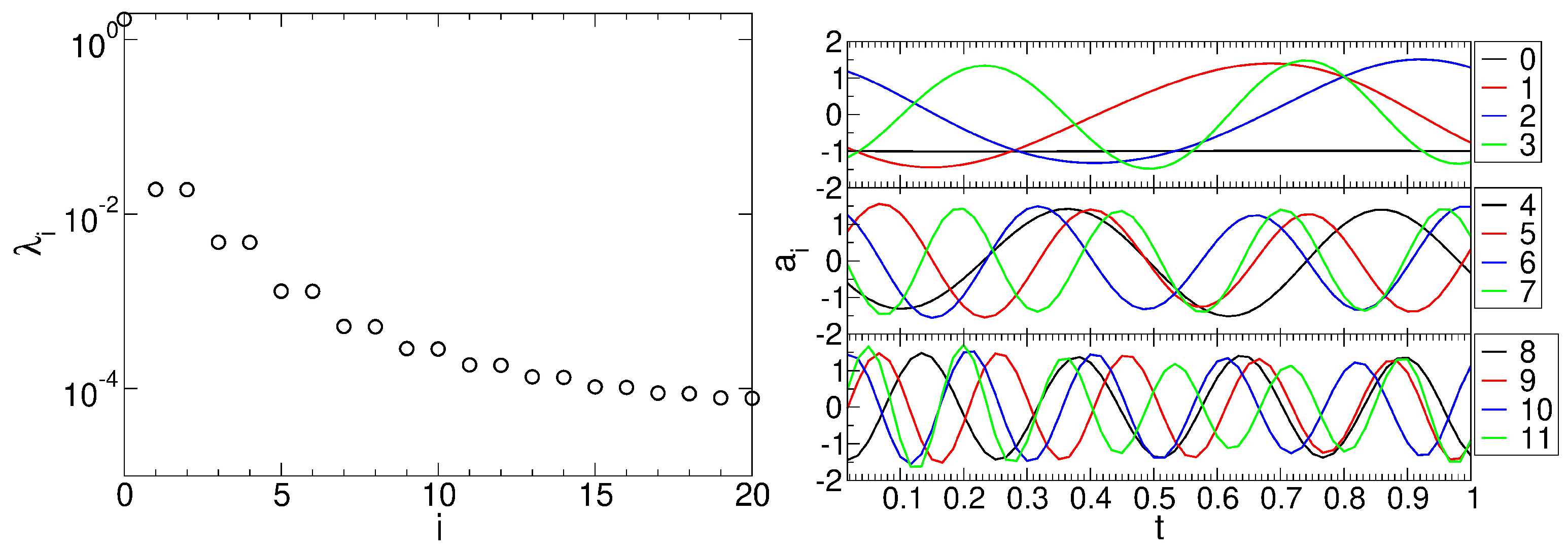
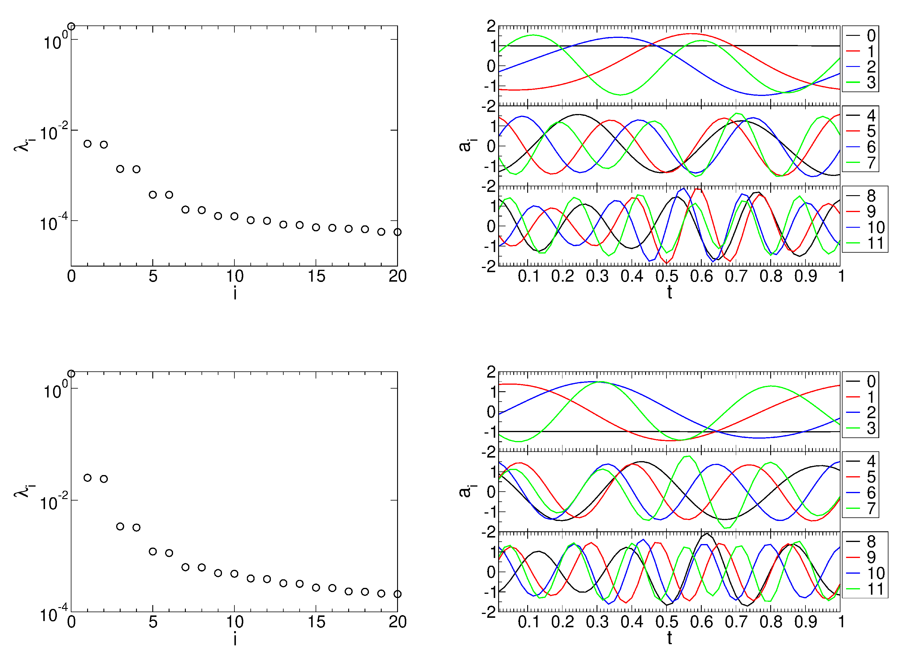
To conclude, large-eddy simulations of a 50% reaction stage and a linear cascade with circular cylinder bar wake generators with two different diameters were carried out for a Reynolds number based on inlet velocity and axial chord length of 50,000. For the this Reynolds number, which is on the low end of what is seen on actual engines, considerable laminar separation from the suction surface and a passage vortex and corner separation lead to high total pressure losses. Because of the large size of the simulations, only a limited number of wake passing periods were simulated and the quality of the phase-averaged data was improved by using the proper orthogonal decomposition as a filter to remove the small-scale high-frequency content.

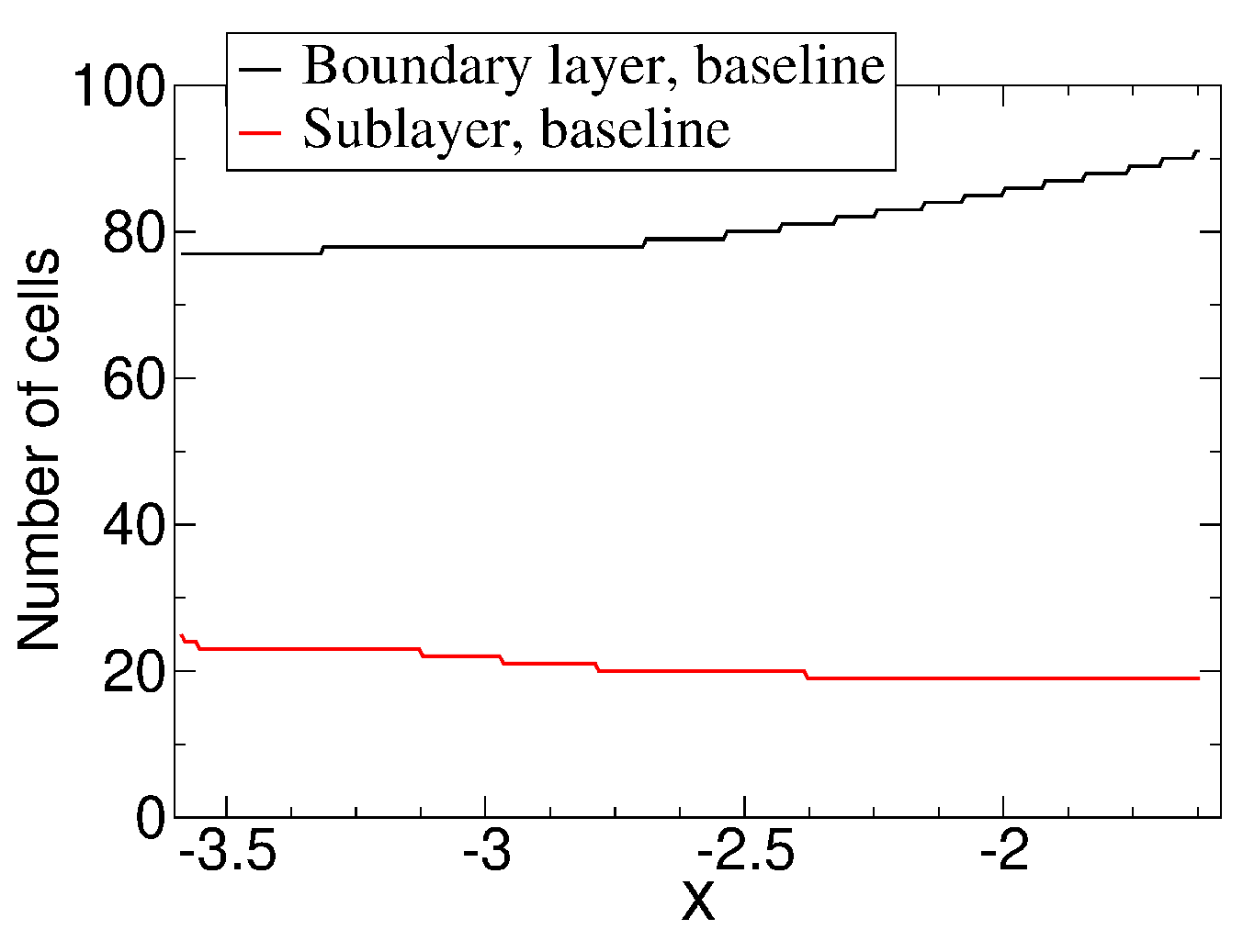
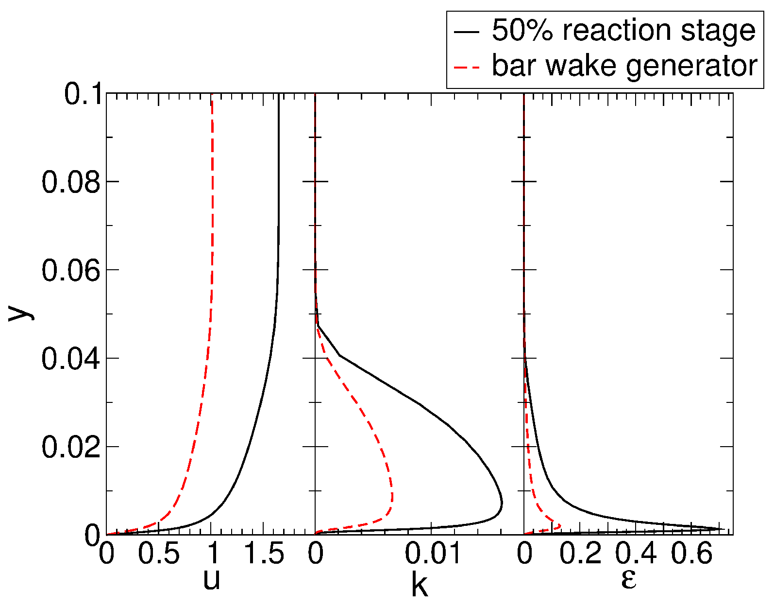
An approach flow analysis revealed that the boundary layer grows much faster for the cases with bar wake generator as a result of the relative motion of the endwall with respect to the freestream. This effect can be avoided by having the bar wake generator extent through a slit in the endwall as is often done in experiments. Because of the low-Reynolds number conditions, the laminar separation from the suction surface of the upstream vane for the 50% reaction stage is substantial, leading to a large wake with considerable velocity deficit.

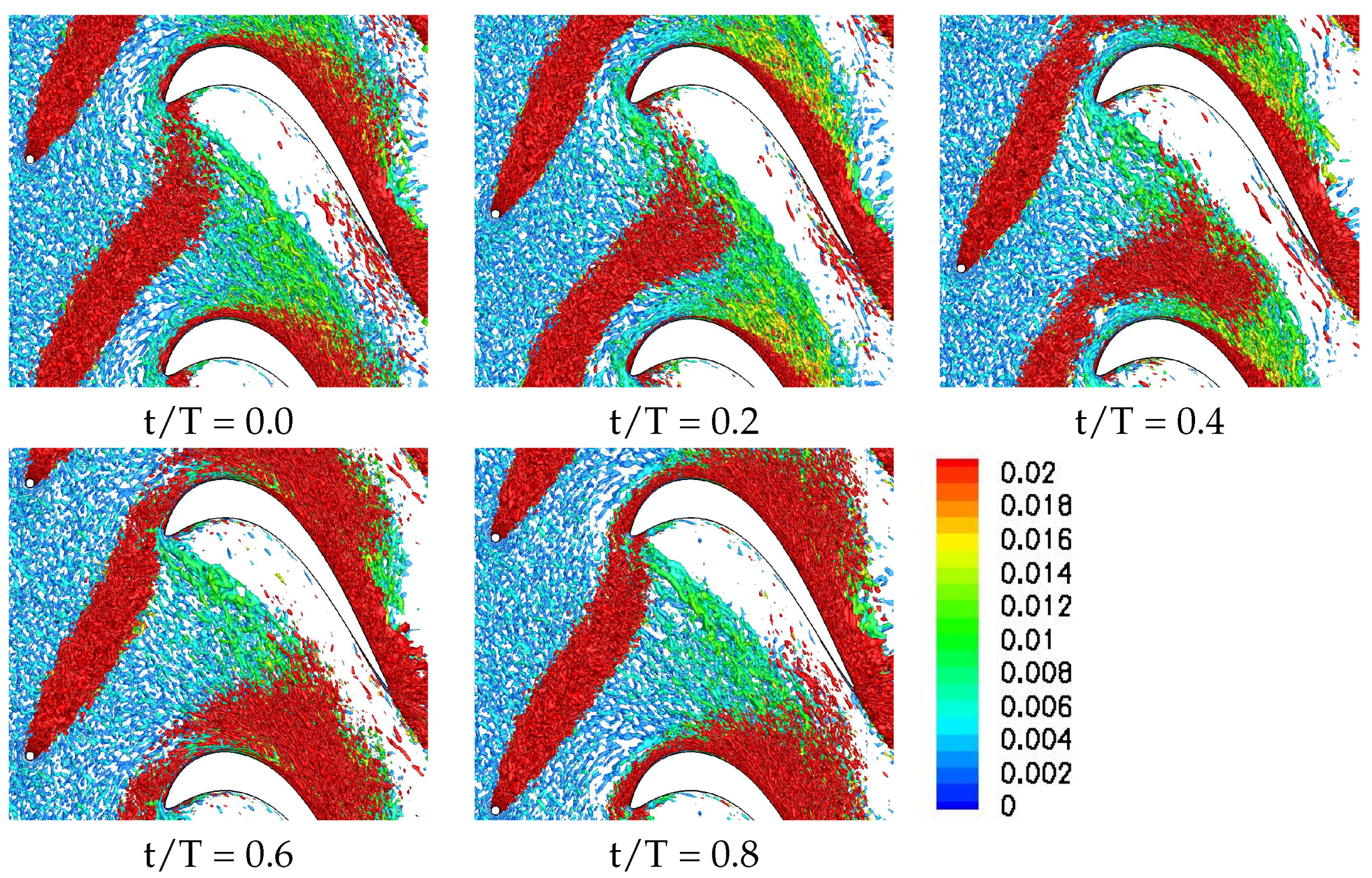
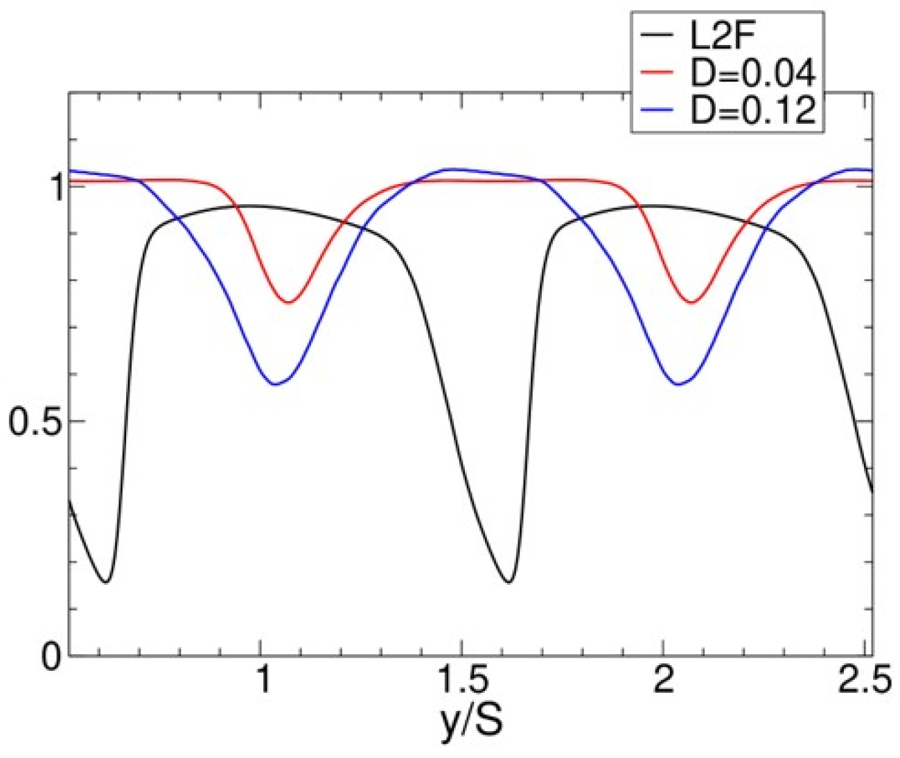
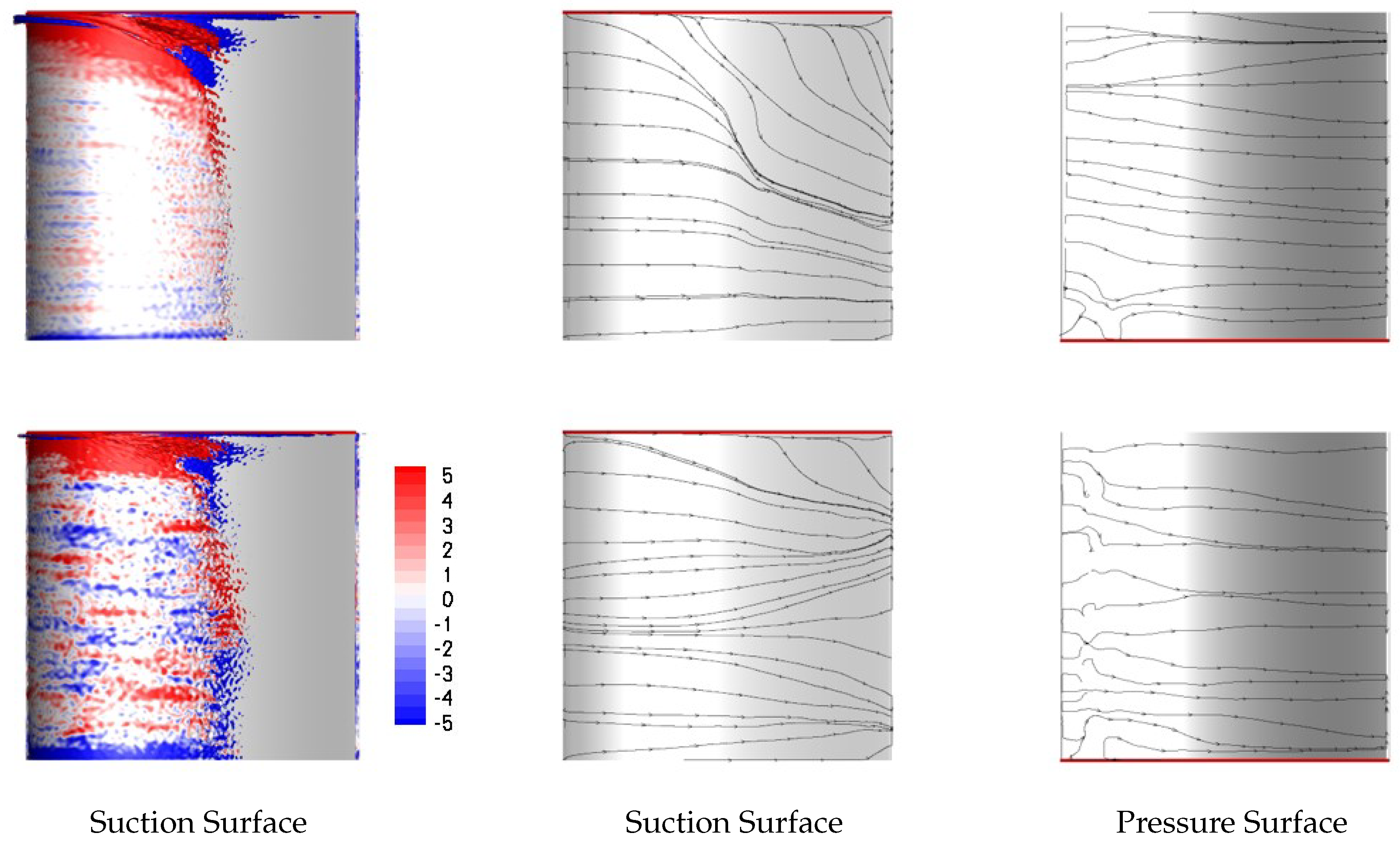
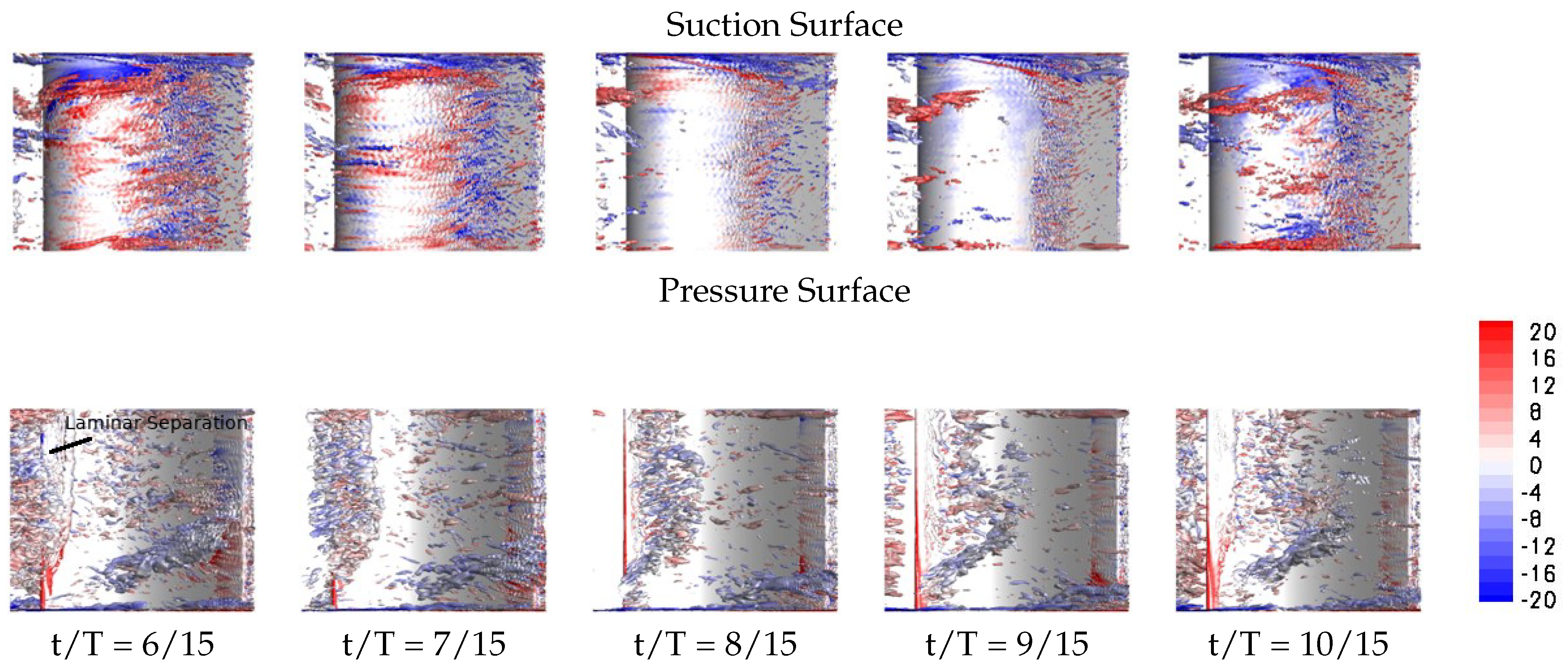
In bar wake generator experiments, the wake generator radius is often of the same order of magnitude as the trailing edge radius of the stator vane. The present simulations indicate that a much larger diameter bar wake generator is needed at Re = 50,000 to match the wake width and integral momentum deficit of the upstream stator vane. Nevertheless, even for the smaller one of the two bar wake generators considered in this paper, the laminar suction side separation is entirely suppressed. The passage vortex, on the other hand is not affected much by the small bar wake generator and only intermittently suppressed by the larger bar wake generator while it is entirely suppressed for the upstream stator vane. In addition, the present results suggest that the elevated endwall losses for front-loaded high-lift airfoils in linear cascade experiments maybe less of a factor in a real turbine environment. Also of interest, for both the large bar wake generator and, even more so, for the upstream stator vane, a laminar separation bubble is generated on the pressure surface near the leading edge.

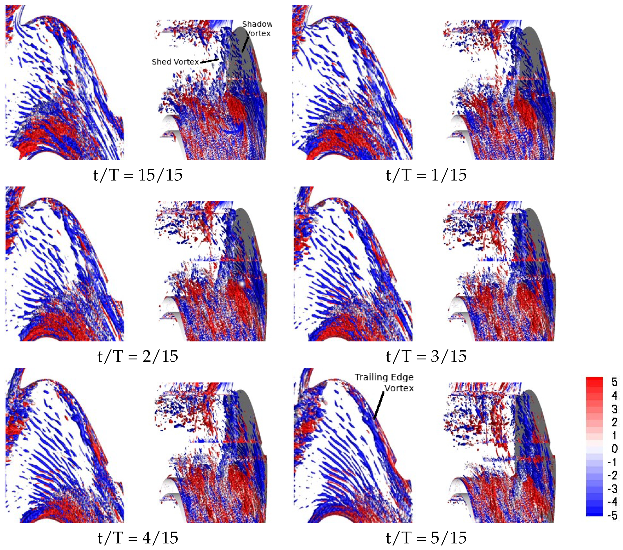
Another major difference between the stator vane wake and the bar wake generator wakes are the strong wake three-dimensionality and pronounced endwall structures for the former. For the stator vane, a new longitudinal structure was observed near the trailing edge of the rotor blade that could be traced back to the near-wall vorticity of the stator vane wake. This structure, which likely also has implications for the endwall losses, is missing for the cases with bar wake generator. The present simulations suggest that the bar wake generator diameter has to be chosen carefully when the effect on the suction side flow separation is investigated. Since bar wake generators do not accurately capture the near-wall wake vorticity of the stator vanes, they are likely not a good choice for investigations aimed at understanding the wake effect on the endwall flow.

References

1. McQuilling, M.W. Design and Validation of a High Lift Low-Pressure Turbine Blade. Ph.D. Dissertation, Wright State University, Dayton, OH, USA, 2007. [Google Scholar]
2. Weiss, A.; Fottner, L. The Influence of Load Distribution on Secondary Flow in Straight Turbine Cascades. J. Turbomach. 1995, 117, 133–141. [Google Scholar] [CrossRef]
3. Zoric, T.; Popovic, I.; Sjolander, S.A.; Praisner, T.; Grover, E. Comparative Investigation of Three Highly Loaded LP Turbine Airfoils–Part I: Measured Profile and Secondary Losses at Design Incidence. In Proceedings of the ASME Turbo Expo: Power for Land, Sea and Air, GT2007-2753, Montreal, QC, Canada, 14–17 May 2007. [Google Scholar]
4. Lyall, M.E.; King, P.I.; Clark, J.P.; Sondergaard, R. Endwall Loss Reduction of High Lift Low Pressure Turbine Airfoils Using Profile Contouring—Part I: Airfoil Design. J. Turbomach. 2014, 136, 081005. [Google Scholar] [CrossRef]
5. Bear, P.; Wolff, M.; Gross, A.; Marks, C.; Sondergaard, R. Secondary Loss Production Mechanisms in a Low Pressure Turbine Cascade. In Proceedings of the 52nd AIAA/SAE/ASEE Joint Propulsion Conference, Salt Lake City, UT, USA, 25–27 July 2016. [Google Scholar]
6. Bear, P.; Wolff, M.; Gross, A.; Marks, C.; Sondergaard, R. Experimental Investigation of Total Pressure Loss Development in a Highly Loaded Low Pressure Turbine Cascade. J. Turbomach. 2017, 140, 031003. [Google Scholar] [CrossRef]
7. Langston, L.S.; Nice, M.L.; Hooper, R.M. Three-Dimensional Flow Within a Turbine Blade Passage. ASME J. Eng. Power 1977, 99, 21–28. [Google Scholar] [CrossRef]
8. Langston, L. Secondary flows in axial turbines—A review. Ann. N. Y. Acad. Sci. Heat Transf. Gas Turbine Syst. 2001, 934, 11–26. [Google Scholar] [CrossRef] [PubMed]
9. Sieverding, C.H. Recent Progress in the Understanding of Basic Aspects of Secondary Flows in Turbine Blade Passages. J. Eng. Gas Turbines Power 1985, 107, 248–257. [Google Scholar] [CrossRef]
10. Wang, H.-P.; Olson, S.J.; Goldstein, R.J.; Eckert, E.R.G. Flow Visualization in a Linear Turbine Cascade of High Performance Turbine Blades. J. Turbomach. 1997, 119, 1–8. [Google Scholar] [CrossRef]
11. Goldstein, R.J.; Spores, R.A. Turbulent Transport on the Endwall in the Region Between Adjacent Turbine Blades. J. Heat Transf. 1988, 110, 862–869. [Google Scholar] [CrossRef]
12. Sharma, O.P.; Butler, T.L. Predictions of Endwall Losses and Secondary Flows in Axial Flow Turbine Cascades. J. Turbomach. 1987, 109, 229–236. [Google Scholar] [CrossRef]
13. Kang, S.; Hirsch, C. Three Dimensional Flow in a Linear Compressor Cascade at Design Conditions. In Proceedings of the ASME International Gas Turbine and Aeroengine Congress and Exposition, ASME-91-GT-114, Orlando, FL, USA, 3–6 June 1991. [Google Scholar]
14. Hodson, H.P.; Dominy, R.G. The Off-Design Performance of a Low-Pressure Turbine Cascade. J. Turbomach. 1987, 109, 201–209. [Google Scholar] [CrossRef]
15. Devenport, W.J.; Simpson, R.L. Time-Dependent and Time-Averaged Turbulence Structure Near the Nose of a Wing-Body Junction. J. Fluid Mech. 1990, 210, 23–55. [Google Scholar] [CrossRef]
16. Robison, Z.; Mosele, J.-P.; Gross, A. Numerical investigation of Turbulent Junction Flow Horseshoe Vortex Dynamics. AIAA J. 2021, 59, 1–16. [Google Scholar] [CrossRef]
17. Gross, A.; Marks, C.; Sondergaard, R. Numerical Investigation of Low-Pressure Turbine Junction Flow. AIAA J. 2016, 55, 3617–3621. [Google Scholar] [CrossRef]
18. Gross, A.; Marks, C.; Sondergaard, R.; Bear, P.; Wolff, J. Experimental and Numerical Characterization of Flow through Highly Loaded Low-Pressure Turbine Cascade. J. Propuls. Power 2018, 34, 27–39. [Google Scholar] [CrossRef]
19. Veley, E.; Marks, C.; Anthony, R.; Sondergaard, R.; Fletcher, N.; Wolff, M. Unsteady Flow Measurements in a Low Pressure Turbine Passage using Surface Mounted Thin Film Sensors. In Proceedings of the 53rd AIAA/SAE/ASEE Joint Propulsion Conference, Atlanta, GA, USA, 10–12 July 2017. [Google Scholar]
20. Veley, E.; Marks, C.; Anthony, R.; Sondergaard, R.; Wolff, M. Unsteady Flow Measurements in a Front Loaded Low Pressure Turbine Passage. In Proceedings of the 2018 AIAA Aerospace Sciences Meeting, Kissimmee, FL, USA, 8–12 January 2018. [Google Scholar]
21. Babcock, H.J.; Reeder, M.; Thomas, L.M.; Marks, C.R. Investigation of Loss Reduction in a High Lift Turbine by Localized Endwall Jets. In Proceedings of the AIAA Propulsion and Energy 2019 Forum, Indianapolis, IN, USA, 19–22 August 2019. [Google Scholar]
22. Romero, S.; Gross, A. Numerical Investigation of Active Flow Control of Low-Pressure Turbine Endwall Flow. J. Propuls. Power 2019, 35, 883–895. [Google Scholar] [CrossRef]
23. Meyer, R.X. The Effect of Wakes on the Transient Pressure and Velocity Distributions in Turbomachines. J. Basic Eng. 1958, 80, 1544–1552. [Google Scholar]
24. Schmitz, J.T.; Perez, E.; Morris, S.C.; Corke, T.C.; Clark, J.P.; Koch, P.J.; Puterbaugh, S.L. Highly Loaded Low-Pressure Turbine: Design, Numerical, and Experimental Analysis. J. Propuls. Power 2016, 32, 142–152. [Google Scholar] [CrossRef]
25. Fletcher, N.; Marks, C.; Sondergaard, R. Characterization of Periodic Unsteadiness Generator for Secondary Flow Studies. In Proceedings of the AIAA Scitech 2019 Forum, San Diego, CA, USA, 7–11 January 2019. [Google Scholar]
26. Fletcher, N.; Wolff, M.; Marks, C.R. Turbine Secondary Flow Response to Upstream Periodic Unsteadiness. In Proceedings of the AIAA Scitech 2020 Forum, Orlando, FL, USA, 6–10 January 2020. [Google Scholar]
27. Schulte, V.; Hodson, H.P. Unsteady Wake-Induced Boundary Layer Transition in High Lift LP Turbines. In Turbo Expo: Power for Land, Sea, and Air, ASME-96-GT-486, Proceedings of the ASME 1996 International Gas Turbine and Aeroengine Congress and Exhibition, Birmingham, UK, 10–13 June 1996; ASME: New York, NY, USA, 1996. [Google Scholar]
28. Schulte, V.; Hodson, H.P. Unsteady Wake-Induced Boundary Layer Transition in High Lift LP Turbines. J. Turbomach. 1998, 120, 28–35. [Google Scholar] [CrossRef]
29. Kaszeta, R.W.; Simon, T.W.; Ashpis, D.E. Experimental Investigation of Transition to Turbulence as Affected by Passing Wakes. In Proceedings of the ASME Turbo Expo: Power for Land, Sea and Air, ASME-GT2001-0195, New Orleans, LA, USA, 4–7 June 2001. [Google Scholar]
30. Wu, X.; Durbin, P.A. Evidence of longitudinal vortices evolved from distorted wakes in a turbine passage. J. Fluid Mech. 2001, 446, 199–228. [Google Scholar] [CrossRef]
31. Michelassi, V.; Wissink, J.; Rodi, W. Analysis of DNS and LES of Flow in a Low Pressure Turbine Cascade with Incoming Wakes and Comparison with Experiments. Flow Turbul. Combust. 2002, 69, 295–330. [Google Scholar] [CrossRef]
32. Michelassi, V.; Wissink, J.G.; Fröhlich, J.; Rodi, W. Large-Eddy Simulation of Flow Around Low-Pressure Turbine Blade with Incoming Wakes. AIAA J. 2003, 41, 2143–2156. [Google Scholar] [CrossRef]
33. Stieger, R.D.; Hodson, H.P. The Transition Mechanism of Highly Loaded Low-Pressure Turbine Blades. J. Turbomach. 2004, 126, 536–543. [Google Scholar] [CrossRef]
34. Stieger, R.D.; Hodson, H.P. The Unsteady Development of a Turbulent Wake through a Downstream Low-Pressure Turbine Blade Passage. J. Turbomach. 2005, 127, 388–394. [Google Scholar] [CrossRef]
35. Nessler, C.; Marks, C.; Sondergaard, R.; Wolff, M. PIV Investigation of Periodic Unsteady Wakes over a Highly Loaded LPT Blade. In Proceedings of the 45th AIAA/ASME/SAE/ASEE Joint Propulsion Conference & Exhibit, Denver, CO, USA, 2–5 August 2009. [Google Scholar]
36. Nessler, C.A. Characterization of Internal Wake Generator at Low Reynolds Number with a Linear Cascade of Low Pressure Turbine Blades. Master’s Thesis, Wright State University, Dayton, OH, USA, 2010. [Google Scholar]
37. Volino, R.J. Effect of Unsteady Wakes on Boundary Layer Separation on a Very High Lift Low Pressure Turbine Airfoil. J. Turbomach. 2011, 134, 011011. [Google Scholar] [CrossRef]
38. Sinkwitz, M.; Winhart, B.; Engelmann, D.; di Mare, F.; Mailach, R. Experimental and Numerical Investigation of Secondary Flow Structures in an Annular LPT Cascade under Periodical Wake Impact—Part 1: Experimental Results. In Proceedings of the International Symposium on Transport Phenomena and Dynamics of Rotating Machinery, Maui, HI, USA, 16–21 December 2017. [Google Scholar]
39. Cui, J.; Rao, V.N.; Tucker, P. Numerical Investigation of Contrasting Flow Physics in Different Zones of a High-Lift Low-Pressure Turbine Blade. J. Turbomach. 2016, 138, 011003. [Google Scholar] [CrossRef]
40. Cui, J.; Rao, V.N.; Tucker, P.G. Numerical investigation of secondary flows in a high-lift low pressure turbine. Int. J. Heat Fluid Flow 2017, 63, 149–157. [Google Scholar] [CrossRef] [Green Version]
41. Romero, S.; Gross, A. Numerical Investigation of Low-Pressure Turbine Stage with Unsteady Wakes. In Proceedings of the AIAA Scitech 2020 Forum, Orlando, FL, USA, 6–10 January 2020. [Google Scholar]
42. Robison, Z.; Gross, A. Numerical Investigation of Low-Pressure Turbine Cascade with Unsteady Wakes. In Proceedings of the AIAA Scitech 2021 Forum, Virtual, online, 11–15 and 19–21 January 2021. [Google Scholar]
43. Gross, A.; Fasel, H.F. High-Order WENO Schemes Based on the Roe Approximate Riemann Solver. In Proceedings of the 32nd AIAA Fluid Dynamics Conference and Exhibit, St. Louis, MO, USA, 24–26 June 2002. [Google Scholar]
44. Gross, A.; Fasel, H.F. High-Order-Accurate Numerical Method for Complex Flows. AIAA J. 2008, 46, 204–214. [Google Scholar] [CrossRef]
45. Romero Martinez, S.R.; Gross, A. Numerical Investigation of Strategies Aimed at Reduction of Low-Pressure Turbine Endwall Losses. In Proceedings of the AIAA Scitech 2019 Forum, San Diego, CA, USA, 7–11 January 2019. [Google Scholar]
46. Jarrin, N.; Benhamadouche, S.; Laurence, D.; Prosser, R. A synthetic-eddy-method for generating inflow conditions for large-eddy simulations. Int. J. Heat Fluid Flow 2006, 27, 585–593. [Google Scholar] [CrossRef] [Green Version]
47. Poletto, R.; Craft, T.; Revell, A. A New Divergence Free Synthetic Eddy Method for the Reproduction of Inlet Flow Conditions for LES. Flow Turbul. Combust. 2013, 91, 519–539. [Google Scholar] [CrossRef]
48. Mankbadi, M.R.; Vyas, M.A.; DeBonis, J.R.; Georgiadis, N.J. Evaluation of Inflow Turbulence Methods in Large-Eddy Simulations of a Supersonic Boundary Layer. In Proceedings of the 2018 Fluid Dynamics Conference, Atlanta, GA, USA, 25–29 June 2018. [Google Scholar]
49. Klein, M.; Sadiki, A.; Janicka, J. A digital filter based generation of inflow data for spatially developing direct numerical or large eddy simulations. J. Comput. Phys. 2003, 186, 652–665. [Google Scholar] [CrossRef]
50. Gross, A.; Fasel, H.F. Multi-block Poisson grid generator for cascade simulations. Math. Comput. Simul. 2008, 79, 416–428. [Google Scholar] [CrossRef]
51. Nicoud, F.; Ducros, F. Subgrid-Scale Stress Modelling Based on the Square of the Velocity Gradient Tensor. Flow Turbul. Combust. 1999, 62, 183–200. [Google Scholar] [CrossRef]
52. Raverdy, B.; Mary, I.; Sagaut, P.; Liamis, N. Large-Eddy Simulation of the Flow around a Low Pressure Turbine Blade. In Direct and Large-Eddy Simulation IV; Geurts, B.J., Friedrich, R., Mt́ais, O., Eds.; ERCOFTAC Series; Springer: Dordrecht, The Netherlands, 2001; Volume 8. [Google Scholar]
53. Gross, A.; Fasel, H.F. Characteristic Ghost-Cell Boundary Conditions. AIAA J. 2007, 45, 302–306. [Google Scholar] [CrossRef]
54. Lumley, J.L. The Structure of Inhomogeneous Turbulent Flows. In Atmospheric Turbulence and Radio Wave Propagation; National Institute of Informatics: Tokyo, Japan, 1967; pp. 166–178. [Google Scholar]
55. Sirovich, L. Turbulence and the dynamics of coherent structures, Part I–III. Q. Appl. Math. 1987, 45, 561–590. [Google Scholar] [CrossRef] [Green Version]
56. Hunt, J.C.R.; Wray, A.A.; Moin, P. Eddies, Stream, and Convergence Zones in Turbulent Flows; Report CTR-S88; Center for Turbulence Research: Stanford, CA, USA, 1988. [Google Scholar]
57. Gross, A.; Marks, C.; Sondergaard, R. Local Spatial Linear Stability Analysis of Low-Pressure Turbine Endwall Boundary Layer. AIAA J. 2018, 56, 2166–2177. [Google Scholar] [CrossRef]
58. Howell, R.J.; Hodson, H.P.; Schulte, V.; Stieger, R.D.; Schiffer, H.; Haselbach, F.; Harvey, N.W. Boundary Layer Development in the BR710 and BR715 LP Turbines-The Implementation of High-Lift Concepts. J. Turbomach. 2002, 124, 385–392. [Google Scholar] [CrossRef]
59. Ciorciari, R.; Kirik, I.; Nielhuis, R. Effects of Unsteady Wakes on the Secondary Flows in the Linear T106 Turbine Cascade. J. Turbomach. 2014, 136, 091010. [Google Scholar] [CrossRef]
Figure 1. RANS profiles.
Aerospace 08 00184 g001
Figure 2. Computational grids for the 50% reaction stage (a) and cascade with bar wake generator with small diameter (b) and large diameter (c). (Reprinted from [42].)
Aerospace 08 00184 g002
Figure 3. Near−wall grid resolutions in wall units.
Aerospace 08 00184 g003
Figure 4. Number of cells within boundary layer ( z δ ) and viscous sublayer ( z + 10 ).
Aerospace 08 00184 g004
Figure 5. Stage velocities for the 50% reaction stage. (Reprinted from [42].)
Aerospace 08 00184 g005
Figure 6. Instantaneous iso−surfaces of Q = 5 colored by streamwise velocity for the 50% reaction stage (top), small bar wake generator (bottom left) and large bar wake generator (bottom right). Red circle highlights streaky structures. (Reprinted from [42].)
Aerospace 08 00184 g006
Figure 7. Time−averaged velocity profiles 1 / 2 C x upstream of stator vane (left) and bar wake generators (right). (Reprinted from [42].)
Aerospace 08 00184 g007
Figure 8. Iso−surfaces of Q = 25 flooded by wall distance ( z > 0.02 is red) for the 50% reaction stage (phase−averaged flow). (Reprinted from [42].)
Aerospace 08 00184 g008
Figure 9. Iso−surfaces of Q = 25 flooded by wall distance ( z > 0.02 is red) for small bar wake generator (phase−averaged flow). (Reprinted from [42].)
Aerospace 08 00184 g009
Figure 10. Iso−surfaces of Q = 25 flooded by wall distance ( z > 0.02 is red) for large bar wake generator (phase−averaged flow). The wakes are considerably wider than for the smaller wake generator (Figure 9). (Reprinted from [42].)
Aerospace 08 00184 g010
Figure 11. Instantaneous iso−surfaces of Q = 25 colored by wall−normal vorticity for the 50% reaction stage (a), small bar wake generator (b), and large bar wake generator (c). The wakes for the bar wake generators exhibit a von Kármán vortex street. (Reprinted from [42].)
Aerospace 08 00184 g011
Figure 12. Iso−contours of streamwise velocity, 0 < u i n < 1 , (top) and streamwise vorticity, 20 < ω i n < 20 , (bottom) for the 50% reaction stage (a), small bar wake generator (b), and large bar wake generator (c) (time-averaged flow). The wake width for the large bar wake generator matches the wake width for the L2F. A strong endwall structure is present for the L2F but not for the bar wake generators. (Reprinted from [42].)
Aerospace 08 00184 g012
Figure 13. Wake profiles of u i n for x = 0.149 averaged over 0.198 < z < 0.791 . (Reprinted from [42].)
Aerospace 08 00184 g013
Figure 14. Iso−surfaces of Q = 25 flooded by 5 < w x < 5 (left) and and iso−contours of 0.01 < c f , x < 0.01 (right) for upstream stator vane of 50% reaction stage (time−averaged flow).
Aerospace 08 00184 g014
Figure 15. Iso−surfaces of Q = 25 flooded by 5 < w x < 5 (left) and skin−friction lines and iso−contours of 0.01 < c f , x < 0.01 (right) for downstream rotor blade of 50% reaction stage (time−averaged flow). Circle marks longitudinal near-wall structures. (Reprinted from [42].)
Aerospace 08 00184 g015
Figure 16. Iso−surfaces of Q = 25 flooded by 5 < w x < 5 (left) and skin−friction lines (right) for the 50% reaction stage. Endwall marked by red line (time−averaged flow). (Reprinted from [42].)
Aerospace 08 00184 g016
Figure 17. Iso−contours of 0.01 < c f , x < 0.01 for suction surface of downstream blade averaged over 0.60 < z < 1 for instantaneous flow for the 50% reaction stage. (Reprinted from [42].)
Aerospace 08 00184 g017
Figure 18. Skin−friction lines on pressure surfaces for the 50% reaction stage for upstream stator vane (a) and downstream rotor blade (b). Endwall marked by red line (time−averaged flow). (Reprinted from [42].)
Aerospace 08 00184 g018
Figure 19. Iso−contours of flow angle at z = 1 for the 50% reaction stage (phase−averaged flow). Arrow marks pressure side flow separation. (Reprinted from [42].)
Aerospace 08 00184 g019
Figure 20. Iso−surfaces of Q = 25 flooded by 5 < w x < 5 (left) and skin−friction lines and iso−contours of 0.01 < c f , x < 0.01 (right) for small bar wake generator (top) and large bar wake generator (bottom) (time−averaged flow). (Reprinted from [42].)
Aerospace 08 00184 g020
Figure 21. Iso−surfaces of Q = 25 flooded by 5 < w x < 5 (left) and skin−friction lines for D = 0.04 (top) and D = 0.12 (bottom) bar wake generators. Endwall marked by red line (time−averaged flow). The bar wake generator wakes suppress the suction surface laminar separation. For the larger bar wake generator, the suction side corner separation is weakened. (Reprinted from [42].)
Aerospace 08 00184 g021
Figure 22. Iso−contours of 0.01 < c f , x < 0.01 for suction surface of downstream blade averaged over 0.60 < z < 1 (phase−averages). For the larger bar wake generator, flow separation is suppressed over the entire period. (Reprinted from [42].)
Aerospace 08 00184 g022
Figure 23. Iso−contours of flow angle at z = 1 for large bar wake generator (phase−averaged flow). Different from the 50% reaction stage, the bar wake generators do not induce flow separation from the pressure side. (Reprinted from [42].)
Aerospace 08 00184 g023
Figure 24. POD eigenvalues and time-coefficients for the 50% reaction stage. (Reprinted from [42].)
Aerospace 08 00184 g024
Figure 25. Reconstructions of phase−averaged flow at t / T = 0 from 5 (left), 10 (center), and 15 (right) POD modes for the 50% reaction stage. Iso−surfaces of Q = 25 flooded by wall distance ( z > 0.02 is red). By including additional modes in the reconstruction, the endwall flow structures are revealed more clearly. (Reprinted from [42].)
Aerospace 08 00184 g025
Figure 26. Iso−surfaces of Q = 25 flooded by wall distance ( z > 0.02 is red) for the 50% reaction stage (phase−averaged flow). POD reconstructions from 15 modes. Longitudinal structure is marked by letter “A”. (Reprinted from [42].)
Aerospace 08 00184 g026
Figure 27. Iso−surfaces of Q = 20 flooded by 5 < w x < 5 for the 50% reaction stage (phase−averaged flow). POD reconstructions from 15 modes. (Reprinted from [42].)
Aerospace 08 00184 g027aAerospace 08 00184 g027b
Figure 28. Iso−surfaces of Q = 10 flooded by 20 < w x < 20 for the 50% reaction stage (phase−averaged flow). POD reconstructions from 15 modes. (Reprinted from [42].)
Aerospace 08 00184 g028
Figure 29. POD eigenvalues and time−coefficients for bar wake generator with D = 0.04 (top) and D = 0.12 (bottom). (Reprinted from [42].)
Aerospace 08 00184 g029
Figure 30. Reconstructions of phase-averaged flow for small bar wake generator. Iso−surfaces of Q = 25 flooded by wall distance ( z > 0.02 is red). POD reconstructions from 15 modes. (Reprinted from [42].)
Aerospace 08 00184 g030
Figure 31. Reconstructions of phase−averaged flow for large bar wake generator. Iso−surfaces of Q = 25 flooded by wall distance ( z > 0.02 is red). POD reconstructions from 15 modes. (Reprinted from [42].)
Aerospace 08 00184 g031
Figure 32. Iso−surfaces of Q = 25 flooded by wall distance, 5 < w x < 5 , for large bar wake generator (phase−averaged flow). POD reconstructions from 15 modes. (Reprinted from [42].)
Aerospace 08 00184 g032