1. Introduction
The study of shock wave attenuation and mitigation is motivated by the serious damage that can be caused by blast waves, both intentional and accidental. This includes explosives as a weapon that can potentially harm soldiers during a war or civilians during a terror attack. Explosives are also used for mining, excavation and demolition. Further, explosions may occur unintentionally, resulting in industrial accidents that damage property and cost lives. With so much at stake, an understanding of how to reduce the energy contained in a blast wave is motivated by more than academic curiosity.
Numerous methods have been investigated to attenuate shock waves. These methods can generally be classified into four groups based on the underlying mechanisms used to reduce the shock strength: (1) the incident shock wave may be diffracted to produce multiple weaker shocks; by distributing the energy of the shock over multiple shocks offset in time, structures impacted by the shock waves experience lower peak pressure; (2) the energy of the shock wave is lost through viscous dissipation of flow kinetic energy; this can be accomplished by creating regions with large velocity gradients, such as boundary layers, jets and wakes; (3) the kinetic energy of the gas may be transferred to barriers and obstacles made of solids or liquids; because the difference in density between a gas and a condensed phase is typically three orders of magnitude, large volumes of gas can be decelerated by a smaller volume of condensed phase mass; and (4) energy can be transferred to the deformation of a condensed phase mass. Examples include deformable and destructible barriers intended to absorb energy, as well as the shearing or vaporization of liquid obstacles. Many shock mitigation techniques feature a combination of one or more of these mechanisms.
A review of the shock wave literature reveals many studies investigating various methods of mitigation. Some methods that have proven effective for this purpose include the introduction of bends inside a duct [
1,
2], the addition of rigid or semi-rigid structures in the path of the shock wave and baffles, orifices, perforated plates with holes or slits, grids and obstacles of varying geometries placed in different patterns [
3,
4,
5,
6,
7,
8,
9,
10,
11].
These methods have proven successful to various degrees and have demonstrated the complex behavior associated with different mechanisms of shock wave mitigation. Of these methods, porous structures featuring pores several orders of magnitude smaller than the diameter of the duct have demonstrated a great deal of promise. The most common examples of such structures are rigid or flexible granular filters [
12,
13,
14] or foams made of solid materials or liquids [
15,
16,
17,
18,
19,
20,
21,
22]. A three-part article series with reviews on the current standing on aqueous foams and experimental observations is presented by Britan
et al. [
15,
16,
17].
Polymer foams, such as polystyrene (one variety of which is sold under the brand name Styrofoam) and polyurethane are widely available and posses properties well suited for use in shock wave experiments. Responses to shock wave loading are dependent on several attributes of the foam, such as the cell structure and foam density, as well as environmental attributes, such as the ambient temperature and humidity. The properties of these foams have been quantified for a range of conditions using experimental methods, such as drop weights, impact sleds, split Hopkinson pressure bars and shock tubes [
23,
24,
25,
26]. The results of these investigations have shown that polymeric foams subjected to high dynamic loads respond first with linear-elastic behavior for small strains. This involves linear bending of the cell walls. Next, the foams displayed elastic buckling and plastic yielding as the strain increases. Finally, the cell walls are crushed, and the collapsed cell matrix starts to deform.
Despite these investigations, a comprehensive understanding of foam properties and how they are coupled to peak pressure and impulse reduction under shock loading is still lacking. Results from shock tube experiments show that foams can be successfully used to mitigate shock waves when placed in front of a surface that it is supposed to protect. One of the more recent experimental works, and perhaps one of the most extensive to date, is that by Seitz and Skews [
22]. In this study, seven different types of foams (with varying foam density, permeability, tortuosity and cell properties) were impacted by shock waves at different strength. The work resulted in a large dataset valuable for the computational simulation community.
In addition to experimental investigations of shock wave attenuation with foam, numerical studies of this method have also been performed. In the work of Ball and East [
27], pressure histories ahead of the exit duct of a shock tube were examined using Lagrangian CFD simulations, for cases in which the duct was obstructed by foam of varying macroscopic geometries. These included semi-infinite and finite length foam sheets and cylindrical foam caps covering the exit duct. There was no significant difference in the attenuation properties of the various geometries. The authors concluded that varying the density of the foams, and therefore, the impedance mismatch of the foam/air interface, had a larger effect on attenuation of blast waves than varying the geometry of the foam or the dimensions of each type of geometry. In 2013, the work of Ram and Sadot [
28] resulted in a constitutive model to predict the pressure history at a shock tube wall behind a foam obstacle. The authors used a single experiment to quantify the foam behavior and were then able to predict its attenuation properties for a wide range of conditions. Ram and Sadot concluded that the pressure history recorded at the wall depended on the incident shock Mach number, the stand-off distance to the wall behind the foam obstacle, the length of the foam obstacle and a lump coefficient that accounts for foam properties. The model was also applied to previous foam attenuation experiments by other research groups (e.g., [
9]), and with success, the new model could predict the results accurately. Ram and Sadot concluded that the geometric shape of the foam obstacle did not influence the pressure history results at the rear wall after experimenting with triangular and cylindrical cross-sectional grids.
In this work, an obstacle made of polymeric foam was inserted in a shock tube to block the path of an incident shock wave. Five differently-shaped obstacles made from two types of foam were used in this study. The geometries consisted of blocks with one, two, three or four convergent shapes, as well as a rectangular block with a flat front face. The types of foam used include Styrofoam brand polystyrene and polyurethane. Data were acquired in the form of pressure traces collected ahead of and behind the obstacles, as well as high-speed schlieren visualization of the shock waves encountering the obstacles. This yielded useful insight into how geometrical properties of the front face of the foam influence the attenuation capabilities. Of particular interest is how the large-scale curvatures of the front face of the foam samples affect the flow.
2. Experimental Setup
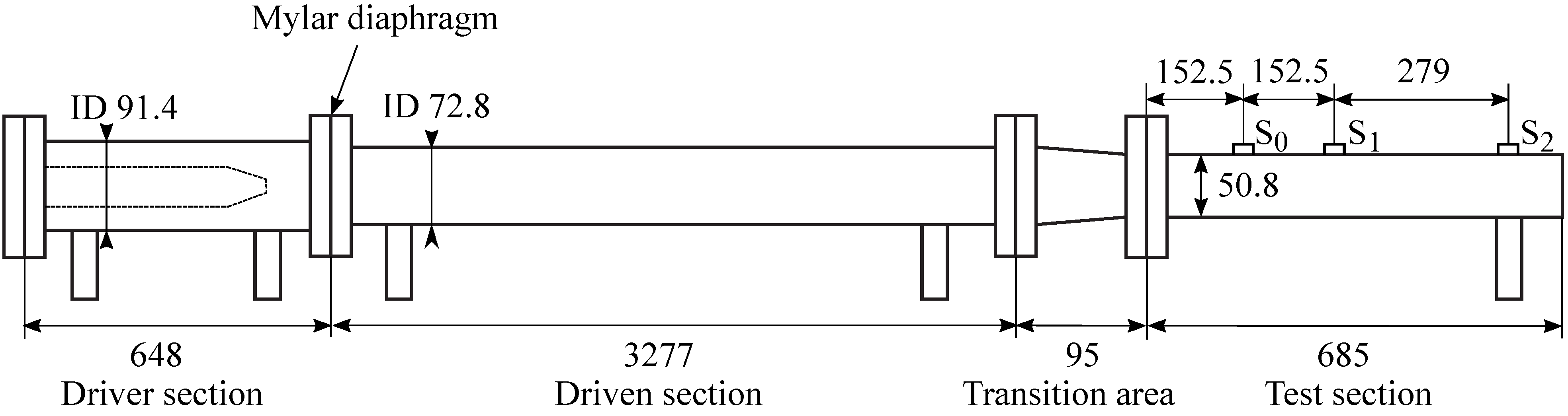
The experiments were performed using a horizontal shock tube; see
Figure 1. The total length of the shock tube setup is 4.7 m with a 0.65 m-long driver section followed by a 3.30 m-long driven section. The inner diameters of the driver and the driven sections are 91.4 and 72.8 mm, respectively, thus leading to a reduction in cross-section area of 37%. The larger size of the driver section produces stronger shocks, and it can also delay the time it takes the reflected expansion wave to reach the driven section [
29,
30]. At the end of the driven section is a transition section, 95 mm long, that transforms the cross-section area from circular to square, while simultaneously also reducing the cross-section area by 38%. A cross-section area reduction increases the shock Mach number. Previous research has shown that a distance of 5–40 diameters is sufficient to produce a planar shock wave front downstream of the membrane location [
31], and hence, it is even shorter for a transition section where a shock wave is already formed. The test section, 685 mm long, is located downstream of the transition section. It is equipped with two sets of windows, one outer polycarbonate pair of windows, 6.4 mm (1/4") thick, and an inner acrylic pair, 3.2 mm (1/8") thick. The inner windows are replaceable to avoid the accumulation of scratches, as samples are pushed through the test section due to the pressure increase of the reflection of the incident shock wave.
Figure 1.
Schematic description of the shock tube. Both the driver and driven sections have circular cross-sections, and the test section has a rectangular cross-section. Three pressure sensors denoted , and are used to measure pressure before and after the foam obstacle. Dimensions in mm; not to scale.
Compressed air was used to fill the driver section while the driven section was left open to atmospheric conditions. Inside the driver section, a device to help break the membrane is placed. It consists of a blade mechanism that is loaded by holding an electromagnet against a permanent magnet with a spring in between with 20 V DC power. This electromagnet insert can reduce non-ideal transient pressure effects inside the shock tube, but it can also decrease the time between incident shock waves and reflected expansion waves reaching the test section [
32]. The electromagnet is covered by a conical head aluminum cover (outer diameter 41.5 mm) to reduce the reflection of the expansion wave. Once the magnet was locked in place, the driver and driven sections were clamped together and separated only by a 50.8 μm-thick Mylar membrane (a polyester film). After the desired pressure differential, 202,016 Pa in the high-pressure section and 101,325 Pa in the low-pressure section, was reached, the power source to the blade mechanism was disconnected, allowing the spring to release the blade, which then pierced the membrane. Pressure was measured by using piezoelectric pressure transducers (PCB 113B21 and 113B31, flush mounted) placed at 152.5, 305 and 584 mm from the beginning of the test section; see
Figure 1. Sensors
and
will be referred to as the upstream and the downstream sensor, respectively, through the rest of this paper.
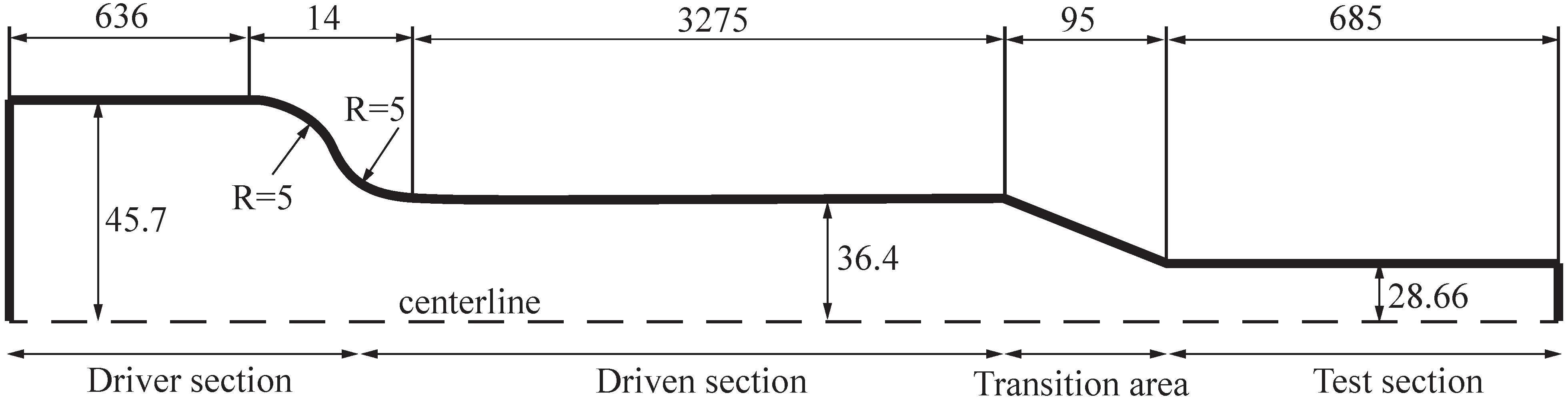
A 3D numerical simulation was used to determine the wave propagation through the shock tube and to produce an
x–
t-diagram. The simulated shock tube has an axisymmetric cylindrical geometry with inner diameters chosen to generate the same cross-section area as in the experimental setup; see
Figure 2. The initial conditions are for a gas at rest with 202,016 Pa in the driver section and 101,325 Pa in the driven, transition and test section. The lengths of the shock tube sections are matched with the experiment. The 3D simulation was conducted using Overture, which is an open-source object-oriented code framework to solve partial differential equations using finite differences on composite grids. More information regarding the solver and the method can be found at
http://www.overtureframework.org/ or in our previous work [
11].
Figure 2.
Schematic of the axisymmetric shock tube used in the simulation. Dimensions in mm; not to scale.
Figure 2.
Schematic of the axisymmetric shock tube used in the simulation. Dimensions in mm; not to scale.
In the simulation, cuboid elements are used to mesh the shock tube. The mesh size of the cuboid elements is 4.7 × 1.5 × 1.5
. The sharp change between the driver and driven sections is rounded using two arcs with a radius of 5 mm. The simulation is solved with the Euler equations of gas dynamics given below.
where
t is the time and
x,
y and
z are the coordinates. The vector of conserved variables
Q is:
where ρ is the fluid density,
u,
v and
w denote the flow velocity in the
x,
y and
z directions and
e is the total energy per unit volume. The flux vectors,
E,
F and
G, are expressed as follows:
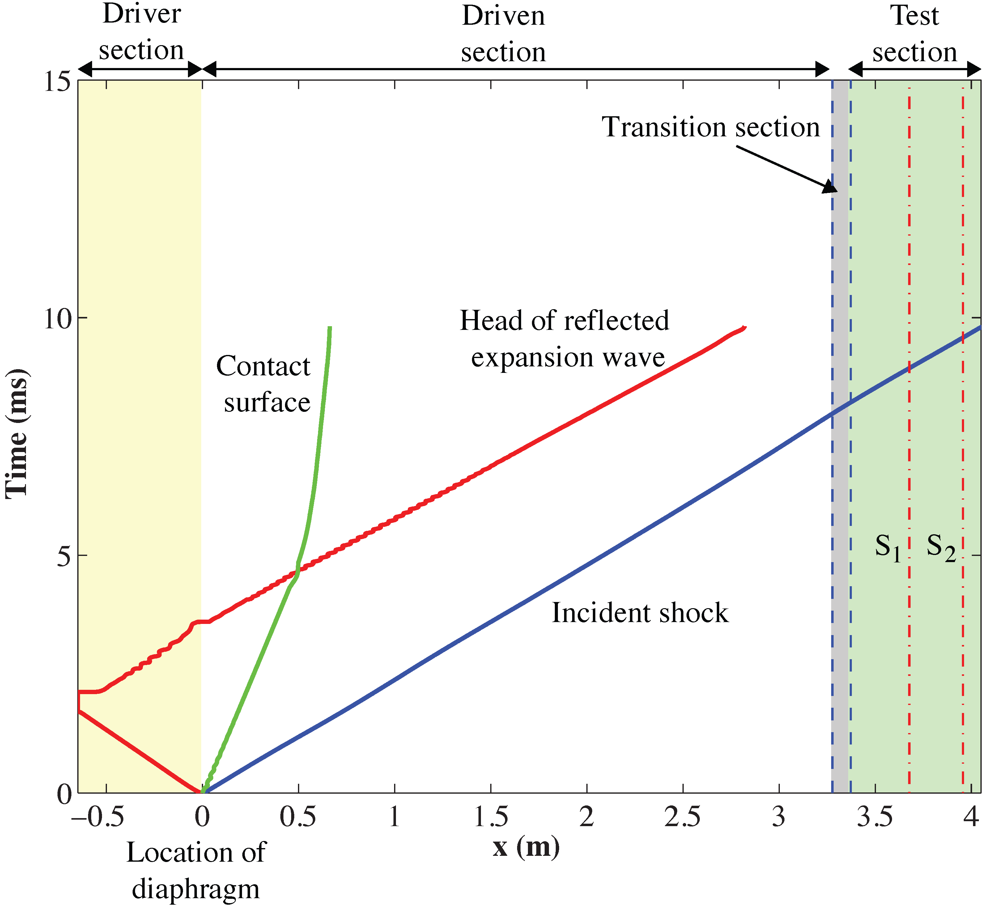
The x–t-diagram shows that the head of the reflected expansion wave arrives at the upstream pressure sensor location (sensor ) after the incident shock wave.
Figure 3.
An x–t diagram showing the incident shock wave, the reflected head of the expansion wave and the contact surface. The driver section is colored yellow, the transition section grey and the test section green. Locations of sensors and are shown with the dashed red lines. The diaphragm is located at m.
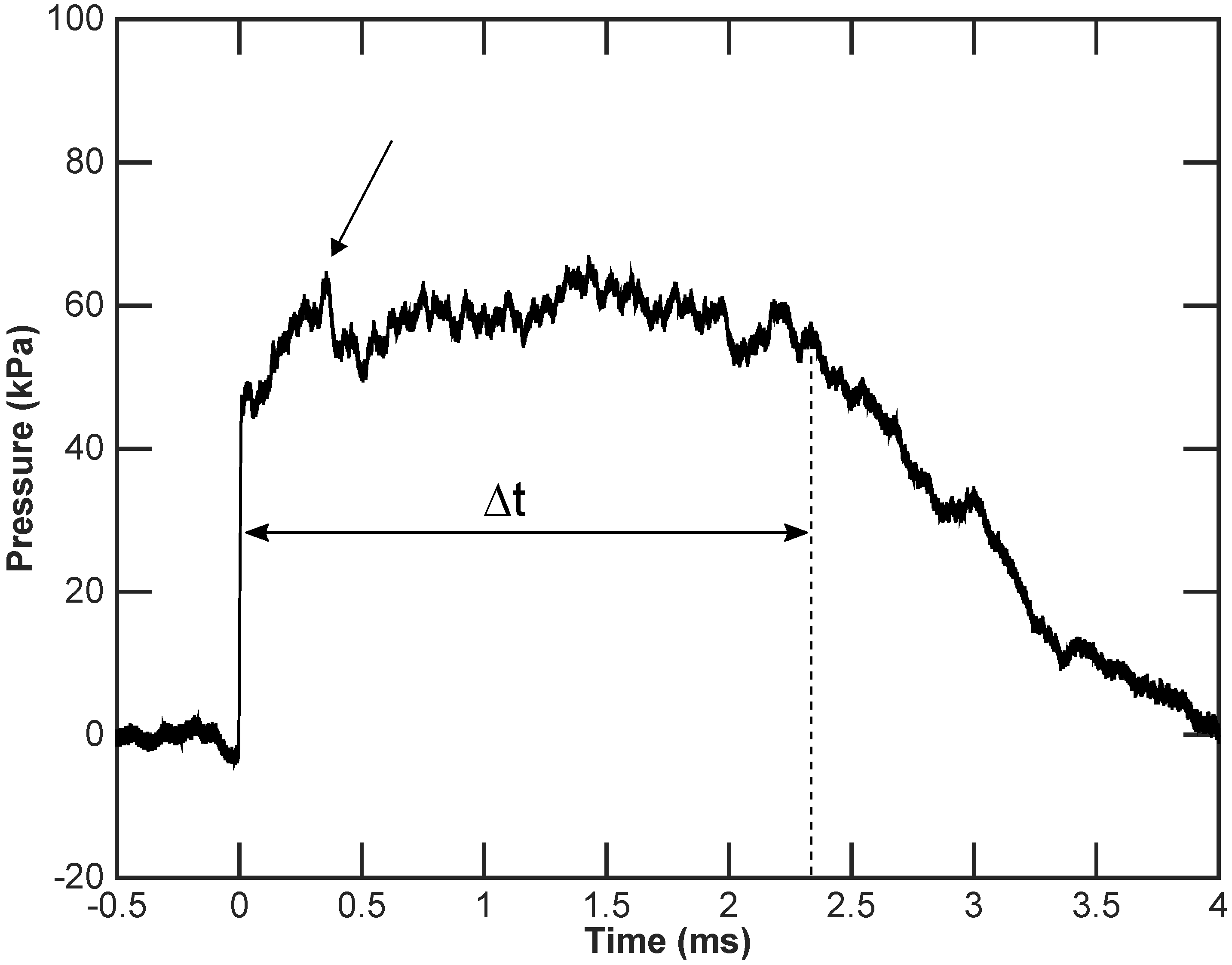
Figure 4 shows a pressure plot obtained from the upstream sensor
mounted in an empty test section. This pressure trace shows a
-ms time interval between the incident shock and the head of the reflected expansion wave. The pressure peak near 0.4 ms in
Figure 4, indicated by the arrow, is caused by weak reflections of a removable panel inside the test section; see the detailed view in
Figure 5. This removable panel is designed to change the samples without causing any deformation of the samples. However, when the samples are inserted into the test section, this panel is covered by the sample, so that this pressure peak does not occur.
Figure 4.
Pressure plot from the upstream sensor with no obstacle in the test section. Time interval ms represents the time between the shock wave and the head of the reflected expansion wave. The arrow points at a reflection caused by a removable panel of the shock tube.
Figure 4.
Pressure plot from the upstream sensor with no obstacle in the test section. Time interval ms represents the time between the shock wave and the head of the reflected expansion wave. The arrow points at a reflection caused by a removable panel of the shock tube.
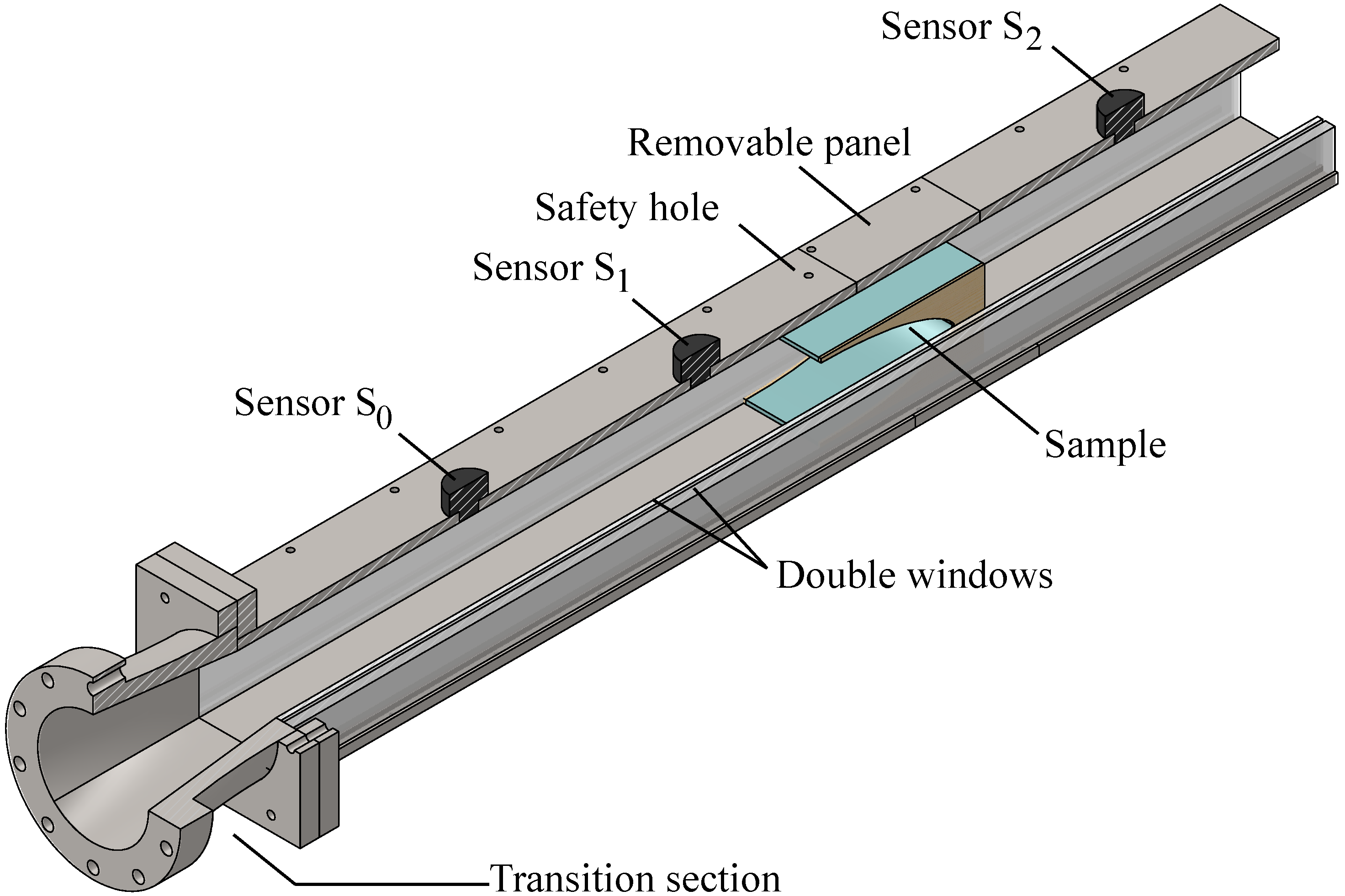
Figure 5.
Sectional view of shock tube test section with transition section, sensor and sample placements.
Figure 5.
Sectional view of shock tube test section with transition section, sensor and sample placements.
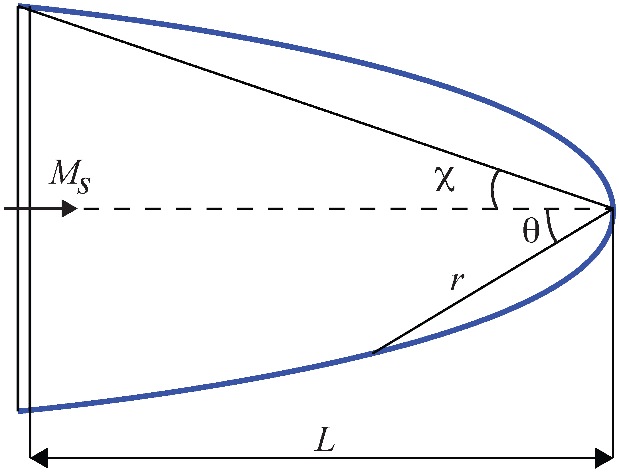
The shapes of the various foam geometries include a logarithmic spiral curve; see
Figure 6. This particular shape was chosen for its previously shown ability to focus a planar incident shock wave towards its focal point using air, as well as water as the shock propagation medium [
34,
35,
36,
37,
38]. The logarithmic spiral curve is given by:
where
L is the characteristic length of the logarithmic spiral,
χ is the characteristic angle and
θ and
r are polar coordinates. The characteristic angle is a function of the incident shock Mach number, and a detailed derivation can be found in, e.g., [
39]. Therefore, given
L,
and the type of gas, the expression for the logarithmic spiral curve can be calculated.
Figure 6.
Logarithmic spiral description. The shock wave propagates from left to right.
Figure 6.
Logarithmic spiral description. The shock wave propagates from left to right.
A Z-folded schlieren system was used to capture photographs of the shock interacting with the foam samples, further described in [
40]. All photographs in this study were obtained using a Phantom V711 camera with a continuous white light source (Cree XLamp, XP-G2 LEDs, Cool White). The camera settings for the various cases are summarized in
Table 1.
Table 1.
Camera settings. Note: the same settings were used for all open cell foam schlieren photographs.
Table 1.
Camera settings. Note: the same settings were used for all open cell foam schlieren photographs.
| Case | Exposure Time | Frame Rate | Resolution |
|---|
| (μs) | (Frames/s) | (mm/pix) |
|---|
| Open cell | 0.38 | 86,075 | 0.387 |
| NC (closed cell) | 0.94 | 210,526 | 0.414 |
| 1C (closed cell) | 0.38 | 150,110 | 0.414 |
| 2C (closed cell) | 0.38 | 210,526 | 0.414 |
| 3C (closed cell) | 0.38 | 210,526 | 0.414 |
| 4C (closed cell) | 0.38 | 210,526 | 0.414 |
2.1. Sample Preparation
Two different types of foams were used: (1) a closed cell polystyrene foam (ASTM C578 Type IV) with a density of 24.8 kg/m
3; and (2) an open cell polyurethane foam with a density of 28.83 kg/m
3 (also known as Aquazone). The densities were obtained from the manufacturer data.
Figure 7 shows a micrograph of the polyurethane foam taken at 40× magnification using a JEOL-JSM 7001 scanning electron microscope (JEOL Ltd., Tokyo, Japan). The top surface of the foam sample was sputtered with platinum coating, and the edges were painted with colloidal graphite to make it conductive. The micrograph shows the foam’s open cell structure, as evidenced by the pores in each cell leading to other cells. Each cell opening is roughly 0.4 mm wide.
Figure 7.
Scanning electron microscope image of the open-celled structure of polyurethane foam.
Figure 7.
Scanning electron microscope image of the open-celled structure of polyurethane foam.
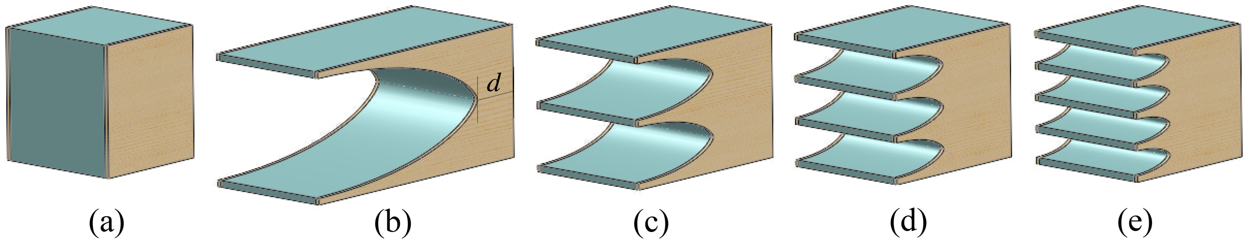
The five different foam samples are shown in
Figure 8. Each sample was constructed using a foam core sandwiched between two 2.54 mm-thick plywood sheets. Each plywood sheet was cut with a laser, and the plywood grains were oriented in the direction of the incident shock wave. The front face of the foam sample,
i.e., the side facing the incident shock wave, was cut into different convergent shapes using a hot wire, and the samples were cut in the same directions from the original foam sheets. Small variations in the front surface occurred due to varying hot wire temperatures and cutting speeds. The plywood was used to prevent the foam from deforming as it was inserted into the test section of the shock tube.
In these experiments, the logarithmic spiral shape was chosen for an incident shock Mach number of
, and depending on the case, the characteristic length was varied to accommodate one, two, three or four curves. To keep the total mass of the foam samples constant, the distance from the focal point of the logarithmic spiral curve to the rear end of the sample,
d, defined in
Figure 8b, was different for all cases. The mass of the Styrofoam samples (without the wood panels) was 3.9 ± 0.2 g, and for the polyurethane samples, it was 3.7 ± 0.1 g. A summary of sample configurations is shown in
Table 2.
Figure 8.
Foam samples: (a) NC; (b) 1C; (c) 2C; (d) 3C; (e) 4C.
Figure 8.
Foam samples: (a) NC; (b) 1C; (c) 2C; (d) 3C; (e) 4C.
Table 2.
Overview of experimental sample configurations.
Table 2.
Overview of experimental sample configurations.
| Case | # of LS | L | d |
|---|
| (–) | (mm) | (mm) |
|---|
| NC | – | – | 47 |
| 1C | 1 | 87 | 20 |
| 2C | 2 | 46 | 33 |
| 3C | 3 | 29 | 37 |
| 4C | 4 | 19 | 39 |
The samples were designed to fill the entire test section with a slight interference fit to not leave any open air gaps for the shock to propagate through, following the experiments presented in [
19]. No visible deformation was found in the samples after insertion in the test section. A sketch of a sample inserted in the test section is shown in
Figure 5 together with the transition section.
3. Results and Discussion
To begin, the shock wave speed was measured using three pressure sensors inserted in the test section. A shock Mach number of
was measured for the experimental conditions used in all cases. Based on the pressure ratio between the driver and the driven section, an analytical shock Mach number of 1.16 can be calculated assuming no losses, which is smaller than the measured Mach number. The reasons are the two cross-section area reductions; the first one between the driver and the driven section and the second one between the driven section and the test section. Through repeated experiments, the shock wave speed was shown to decrease no more than 1.8% between the first and the last sensor placed 279 mm apart. This decrease is caused by two open holes in the test section, placed ahead of the foam sample for safety reasons (see the location in
Figure 5).
Figure 9,
Figure 10,
Figure 11,
Figure 12 and
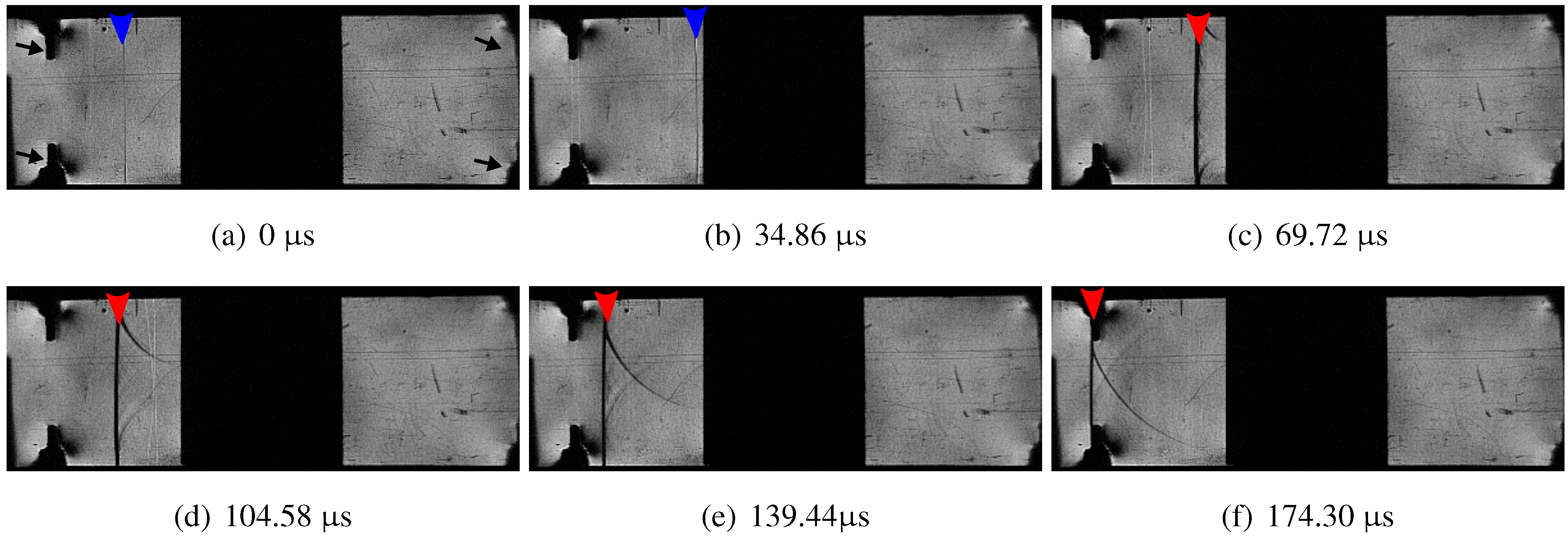
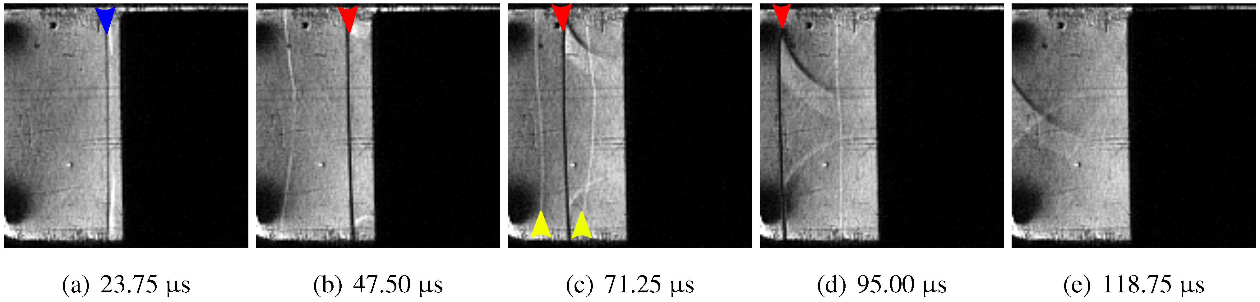
Figure 13 show schlieren photographs for the open cell foam experiments. In these plots, the incident and reflected shock wave fronts are annotated with blue and red arrows, respectively. Case NC is shown in
Figure 9. The incident shock is close to planar with only a two-pixel difference (0.387 mm/pix) between the middle section and the top and bottom sections. This is also true for the reflected shock, which has a slight convex shape with only a two-pixel deviation from a straight line. Additionally, reflections from the upper and lower sides are visible in the photographs.
The deflection of the inner pair of acrylic windows of the test section was estimated and turned out to result in a minimal cross-section area change. Using an approximation of a distributed pressure loading of a simple beam, the bending of the inner acrylic window of the test section has been estimated using the maximum pressure behind the reflected shock. Using these methods, the maximum window deflection under the reflected wave pressure was calculated as 1.37 mm (0.054"). A trapezoidal approximation was then made to calculate the new cross-section area given this deflection. Under the maximum pressure from the reflected wave, the change of the cross-sectional area was found to be approximately 3.6%. This effect could result in a convex reflected shock wave.
However, it is of importance to note that since all samples were tested using the same experimental setup and approach, a comparison of results is valid because all samples encountered the same testing conditions.
The black arrows marking dark regions in
Figure 9a show locations where screws are drilled into the outer windows of the shock tube. Recall that the flow is only in contact with the inner windows, so while minute deformation of the outer windows affects the image captured by the camera, it does not affect the flow.
Figure 9.
Open cell foam, Case NC.
Figure 9.
Open cell foam, Case NC.
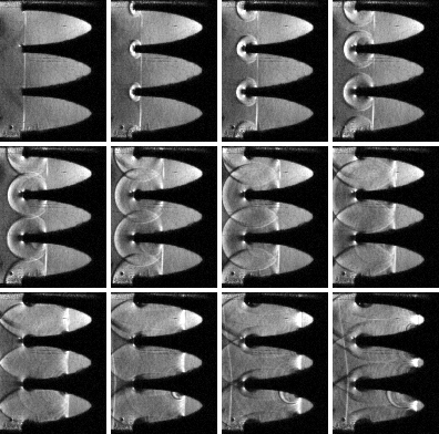
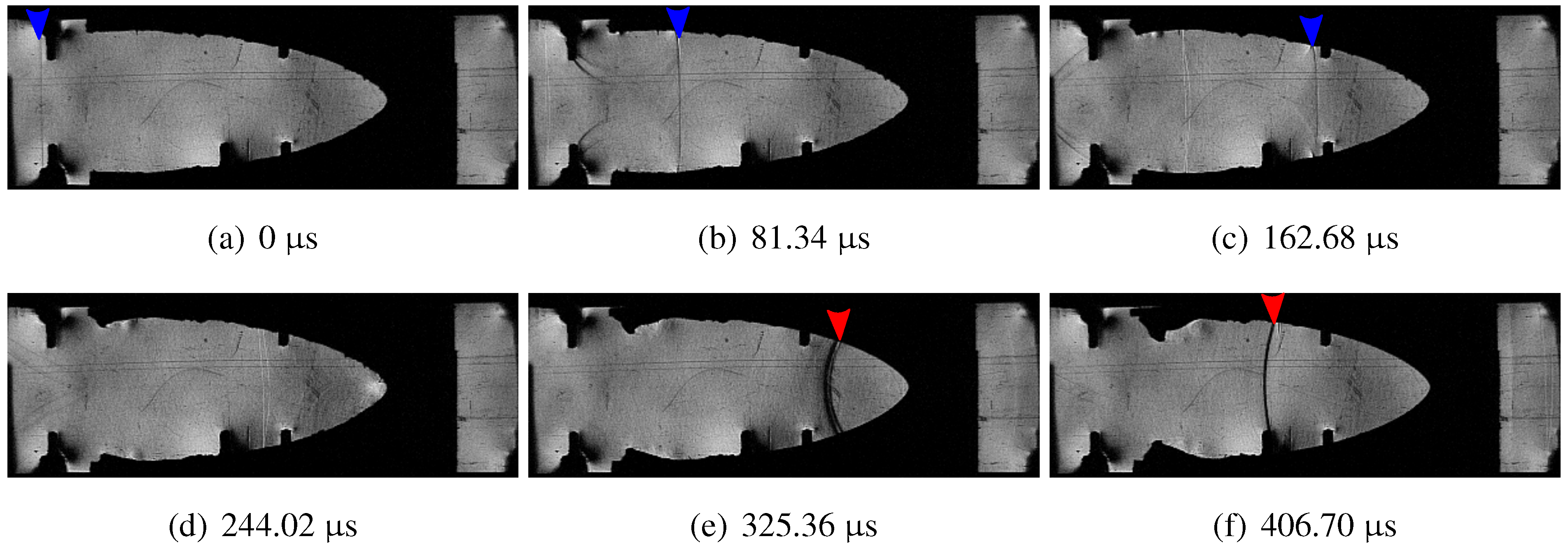
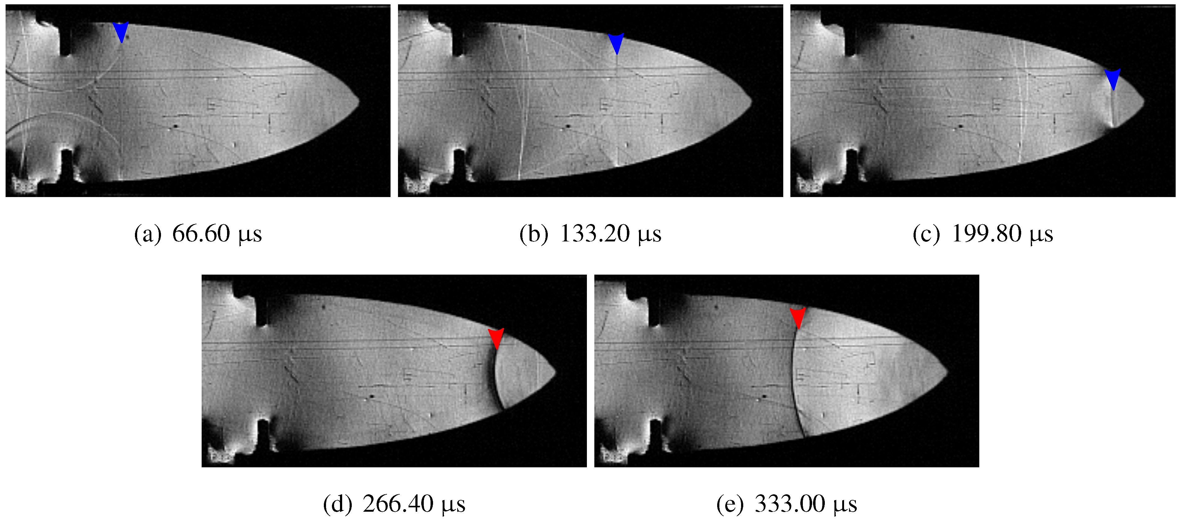
Schlieren photographs of the case with a single logarithmic spiral, Case 1C, is shown in
Figure 10. The front edges of the foam start to deform, clearly visible in
Figure 10c–f. The foam is pulled along with the flow behind the shock wave.
Schlieren photographs of the case with two logarithmic spirals, Case 2C, is shown in
Figure 11. A similar behavior is observed as in the 1C case: the upper and lower edges of the foam are pulled inwards by the flow behind the shock wave. The center piece remains close to its original shape initially and generates a cylindrical shock wave centered on the tip of the center piece. At later times,
Figure 11e–f, the front of the center piece is compressed and becomes blunt.
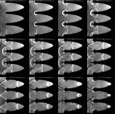
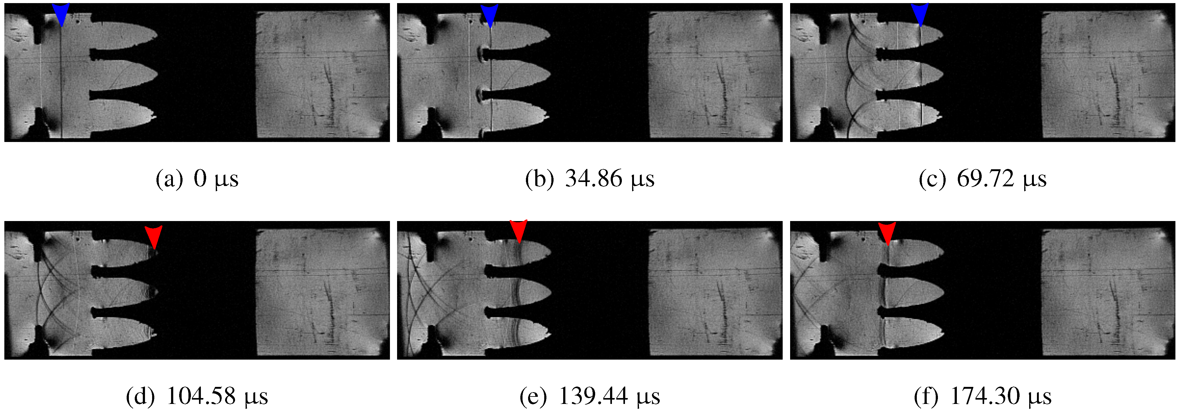
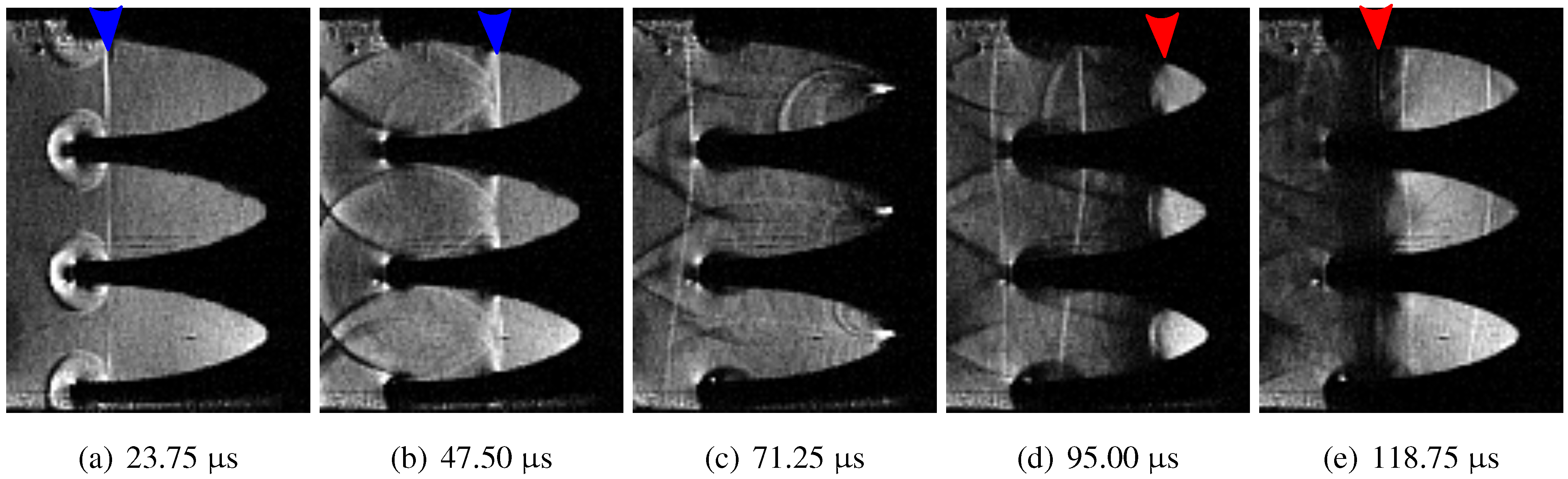
Schlieren photographs of the case with three logarithmic spirals, Case 3C, is shown in
Figure 12. The upper and lower edges, and the center sections where the logarithmic spirals meet cause cylindrical reflected shock waves.
Schlieren photographs of the case with four logarithmic spirals, Case 4C, is shown in
Figure 13. As in the previous cases, cylindrical reflected shock waves are generated. The reflected cylindrical shock waves coalesce into a shock front that becomes planar sooner than the previous cases; see
Figure 13c,d. The reflection from the shock wave that entered the logarithmic spiral curves (red arrows) also coalesces, as it exits the foam sample; see
Figure 13e.
Figure 10.
Open cell foam, Case 1C.
Figure 10.
Open cell foam, Case 1C.
Figure 11.
Open cell foam, Case 2C.
Figure 11.
Open cell foam, Case 2C.
Figure 12.
Open cell foam, Case 3C.
Figure 12.
Open cell foam, Case 3C.
Figure 13.
Open cell foam, Case 4C.
Figure 13.
Open cell foam, Case 4C.
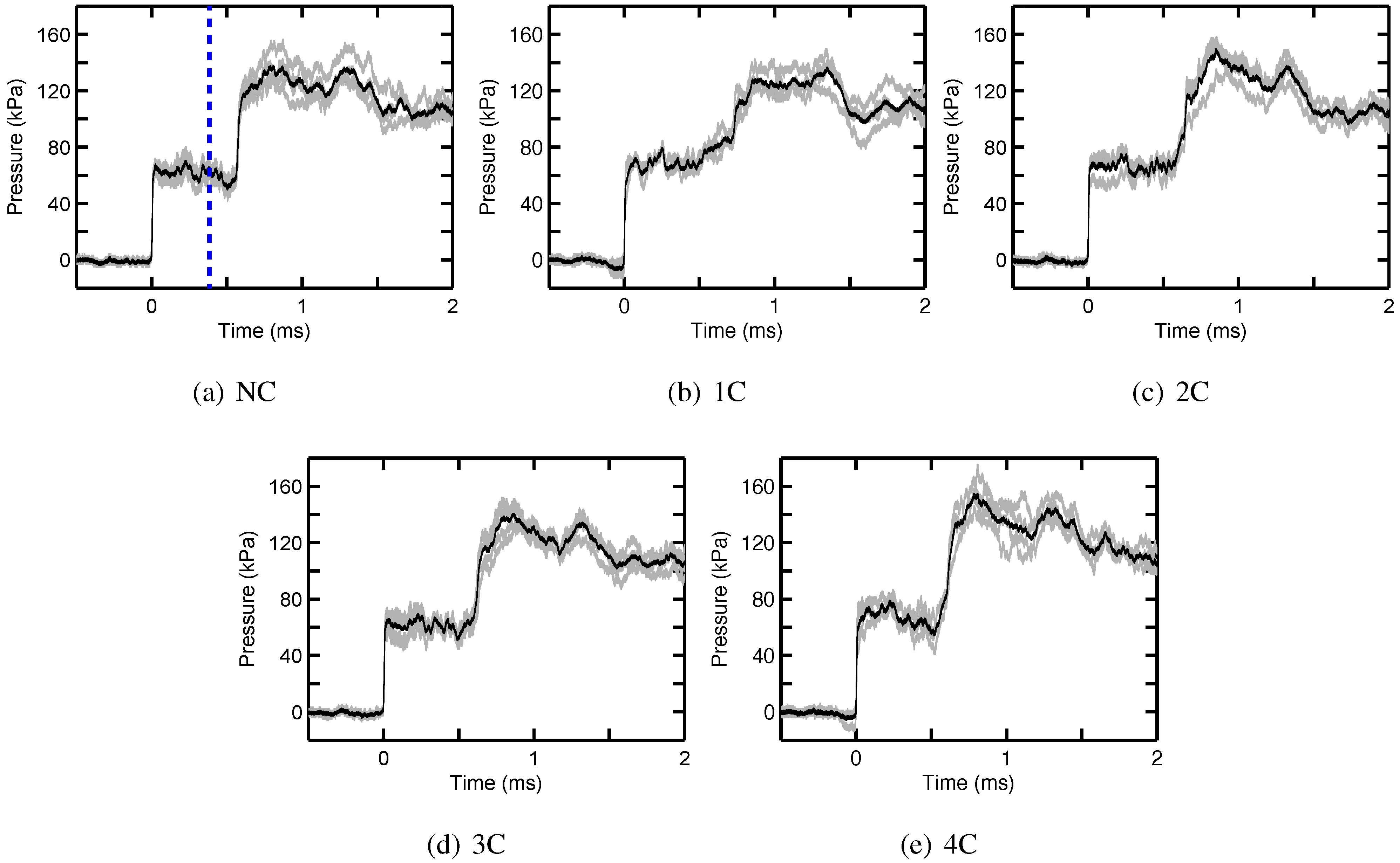
Pressure traces for the incident and reflected waves are shown in
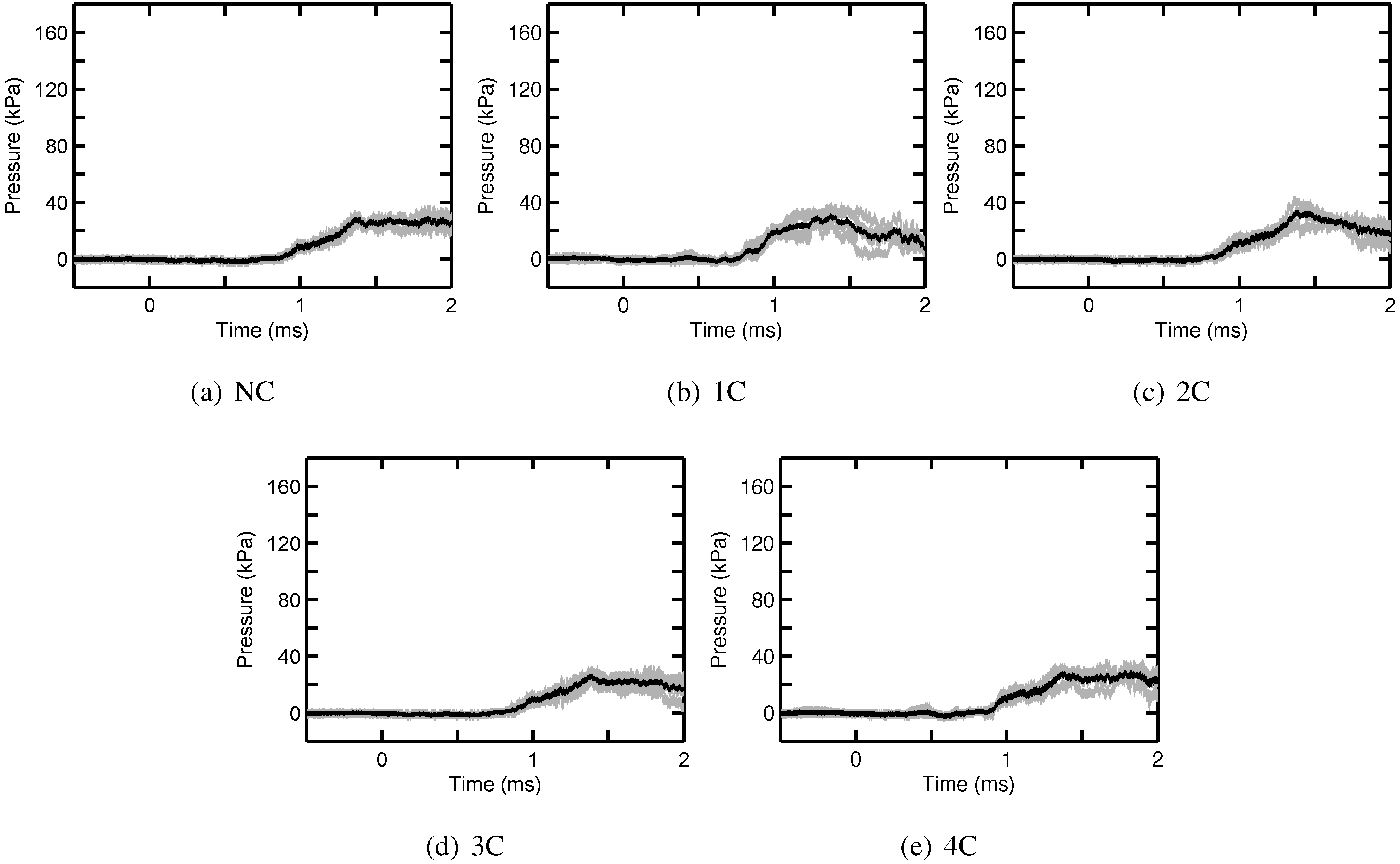
Figure 14 for the five different configurations. The transmitted pressure wave through the different foam specimens is shown in
Figure 15. In these pressure plots, raw temporal profiles of the pressure traces obtained from four or five repeated experiments are shown in gray, and the average is represented by the solid black line. The scatter in the experimental data is too large to conclude if there is a significant difference between the different cases. In
Figure 14a, the blue dotted line represents the approximate time when the foam sample starts to translate, and thus, the pressure upstream of the sample is reduced.
Figure 14.
Open cell foam pressure recordings for all cases: incident and reflected shock.
Figure 14.
Open cell foam pressure recordings for all cases: incident and reflected shock.
Figure 15.
Open cell foam pressure recordings for all cases: transmitted wave.
Figure 15.
Open cell foam pressure recordings for all cases: transmitted wave.
The transmitted wave is not a shock wave, but rather a weak compression wave due to downstream translation of the open cell foam block occurring at about 450 μs.
4. Conclusions
Both the open cell and closed cell foam samples show similar trends in the downstream pressure data, rising at approximately 1 ms. In these experiments, the closed cell and open cell samples begin to translate to downstream in the shock tube at about 350 and 450 μs, respectively. A comparison between open and closed cell foam samples is shown in
Figure 16.
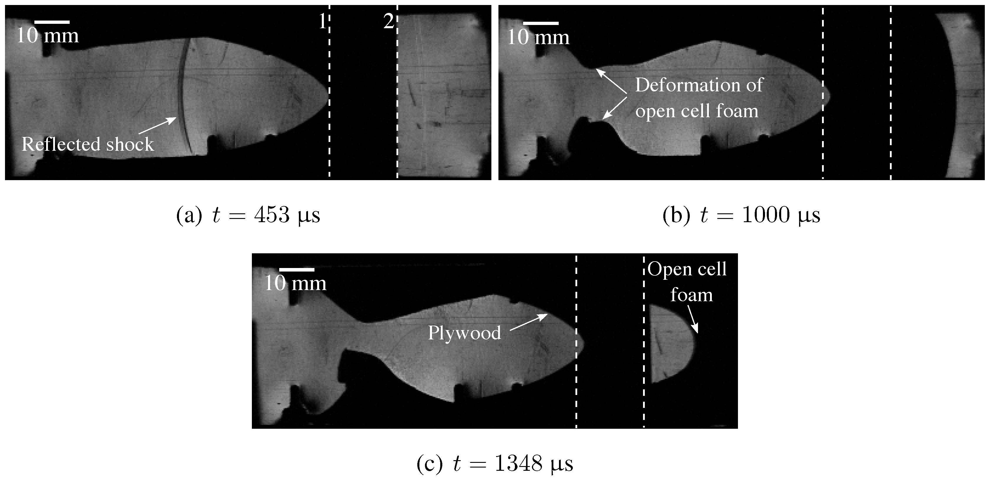
The displacement of the samples creates a compression wave that propagates downstream, thus reducing the pressure upstream of the sample. An example of the translation and deformation of the 1C open cell foam sample is shown in
Figure 17. The foam core moves faster downstream than the plywood sidewalls; see
Figure 17c.
Figure 16.
Photographs showing translation of the NC open and closed cell foam sample. The dashed Lines 1 and 2 represent the original locations of the front and the rear end of the foam block, respectively. (a) s, both samples; (b) s (closed foam), s (open foam); (c) s (closed foam), s (open foam).
Figure 17.
Photographs showing translation and deformation of the 1C open cell foam sample. The dashed Lines 1 and 2 represent the original locations of the tip of the logarithmic spiral and the end of the foam block, respectively.
Figure 17.
Photographs showing translation and deformation of the 1C open cell foam sample. The dashed Lines 1 and 2 represent the original locations of the tip of the logarithmic spiral and the end of the foam block, respectively.
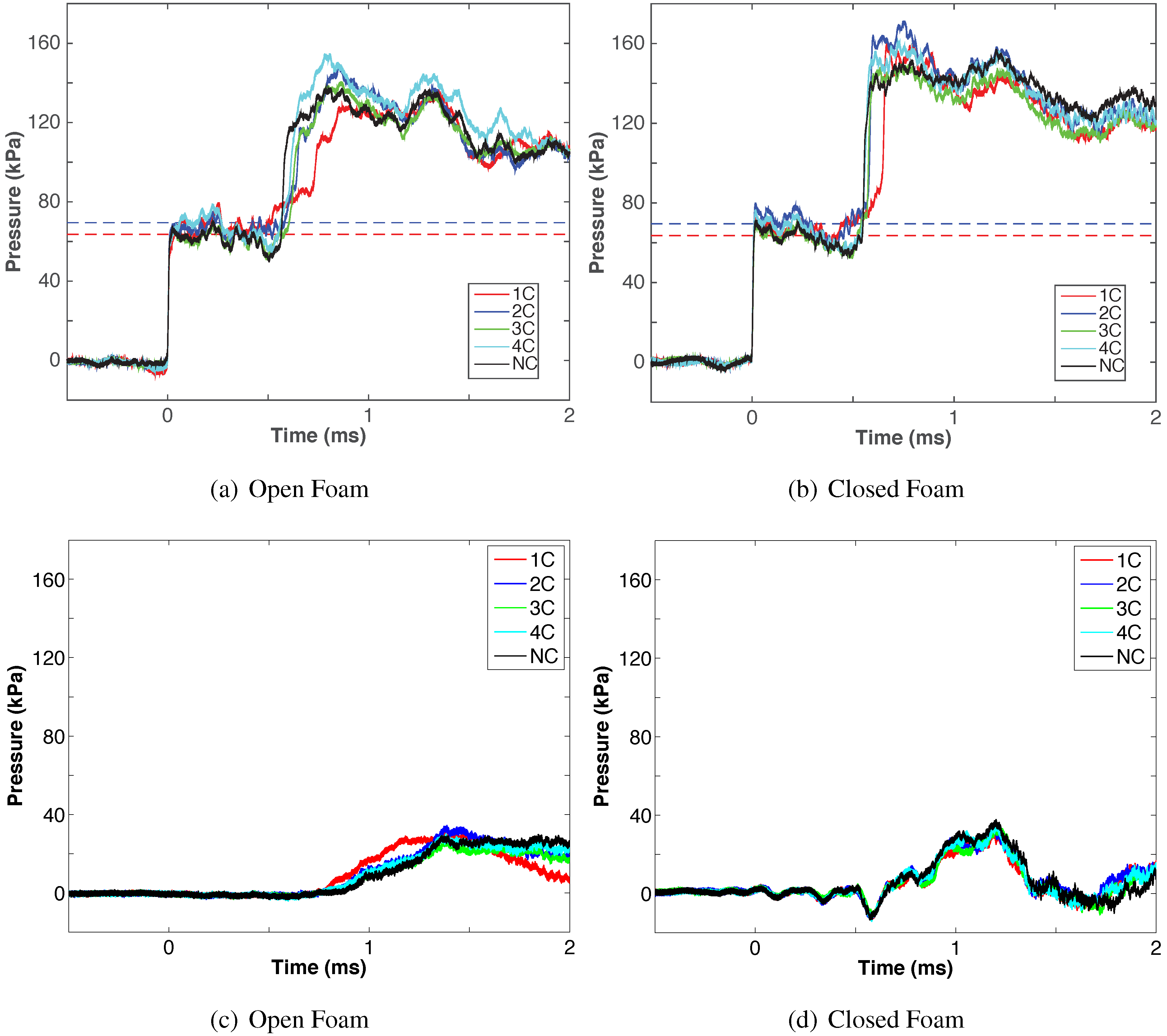
To compare the five different cases for both the open and closed foams, averaged pressure profiles from each case are plotted in
Figure 18. The top row shows the incident and reflected pressures. Dotted lines correspond to the analytical pressure for incident shock waves corresponding to the experimentally measured Mach number
. The bottom row shows the averaged pressure profiles for the downstream sensor
. As a result of the downstream translation of the samples shown in
Figure 16 and
Figure 17, the pressure behind the incident and reflected shocks decreased for all cases; see
Figure 18a,b. The pressure of the closed cell samples decreased sooner than that of the open cell samples, because the closed cell samples experienced earlier translation. A small contribution of the pressure drop is due to the safety hole upstream of the sample; see the hole location in
Figure 5. Apart from that, there are only minor differences between the various cases, or between the open and closed cell foam. Shock attenuation by the foams examined in this study seems to be nearly independent of geometry and porosity; however, the acoustic impedance of the closed cell foam is likely lower than that of the open cell foam, and yet, reflected shock strengths are nearly alike. A time lag between the time of arrival of the reflected wave for different geometries is observed. This is due to the varying lengths of the logarithmic spirals resulting in different travel times for the shock waves.
An artificial negative pressure reading was observed before the incident shock wave in
Figure 18a and also for the compression wave in
Figure 18d. The source of this negative pressure was determined to be the result of a small variation in the construction of the threaded Delrin adapter used to connect the transducers to the shock tube test section. Additional tests showed that the reading of the positive pressure was otherwise accurate and comparable with the results of the other Delrin adapters. The artificial negative pressure is also apparent in
Figure 14b,e and
Figure A7.
Figure 18.
Comparison between open cell and closed cell. Top row: (a) and (b) show the incident and reflected shock wave. The dashed lines show analytical solutions for the range of Mach numbers measured in the experiment. Bottom row: (c) transmitted compression wave; (d) “piston like” driven compression wave.
The results can be concluded as follows:
The pressure magnitudes of the incident shock wave, , were obtained by high-speed image processing and are close to the analytical results. The reflected shock waves were not compared to the analytical results, since the open and closed cell samples were not fixed inside the shock tube and moved after impact.
The experiments were repeated four to five times for each case, but no significant difference was observed within the results from the five different geometry cases, except the time lag. As was previously concluded by Ram and Sadot [
28], the geometry of the obstacles does not influence the degree of attenuation.
The type of foams explored in this study seem to influence the reflected shock wave. The rounding of the pressure pulse of the reflected shock wave in the case of the open cell foam,
Figure 18a, can be attributed to a longer time for shock coalescence, also noted in [
41]. It is noted that the strength of the reflected wave is considerably weaker than the closed cell foam.
Different types of downstream pressure trends are shown in
Figure 18c,d. In the case of the closed cell, there is only “piston like” driven compression wave and edge effects. However, the well-known transmitted compression wave phenomena [
18,
19] were found in the open cell caused by its porosity and permeability, even though it was attenuated by the complex geometry of the open cell foam. The strength of the transmitted compression waves will increase corresponding to increased incident shock wave speed.


 ,
, 
