Turbulence Modeling of Flows with Extensive Crossflow Separation

Abstract

The reasons for the difficulty in simulating accurately strong 3-D shock wave/turbulent boundary layer interactions (SBLIs) and high-alpha flows with classical turbulence models are investigated. These flows are characterized by the appearance of strong crossflow separation. In view of recent additional evidence, a previously published flow analysis, which attributes the poor performance of classical turbulence models to the observed laminarization of the separation domain, is reexamined. According to this analysis, the longitudinal vortices into which the separated boundary layer rolls up in this type of separated flow, transfer external inviscid air into the part of the separation adjacent to the wall, decreasing its turbulence. It is demonstrated that linear models based on the Boussinesq equation provide solutions of moderate accuracy, while non-linear ones and others that consider the particular structure of the flow are more efficient. Published and new Reynolds Averaged Navier–Stokes (RANS) simulations are reviewed, as well as results from a recent Large Eddy Simulation (LES) study, which indicate that in calculations characterized by sufficient accuracy the turbulent kinetic energy of the reverse flow inside the separation vortices is very low, i.e., the flow is almost laminar there.

1. Introduction

Turbulence modeling is one of the most challenging problems in numerical flow simulation. It is common experience that different turbulence models result in different predictions, when applied to a particular complex flow. It is doubtful whether a universally valid turbulence model, capable of describing all complex flows, could be devised. Most of the turbulence models are based on the Boussinesq hypothesis, according to which the apparent turbulent shear stresses are related linearly to the rate of mean strain through an apparent scalar turbulent or “eddy” viscosity coefficient, μ_t. However, in strongly separated flows, the actual dependence of the modeled turbulent shear stresses to the mean strain is non-linear. For alleviating this problem, various non-linear corrections have been devised. In general, non-linear models perform better than linear ones. Still, in many practical aerospace configurations, the accuracy of Reynolds Averaged Navier–Stokes (RANS) simulation results is not satisfactory. Higher order schemes, which do not require a turbulence model for closing the equations, have been developed. The present day computing power is sufficient for the application of Large Eddy Simulation (LES) to simple configurations, like those examined in the present study, although the simulated Reynolds numbers are still rather low. Guidance to modeling of LES is provided by the more computing power demanding Direct Numerical Simulation (DNS). Nevertheless, RANS calculations will continue for many years to support the aerospace industry. Even when LES reach the level of application in aerospace components or complete configurations, it will be more economic to apply RANS in an optimization procedure and subsequently to simulate the optimum configuration by LES.

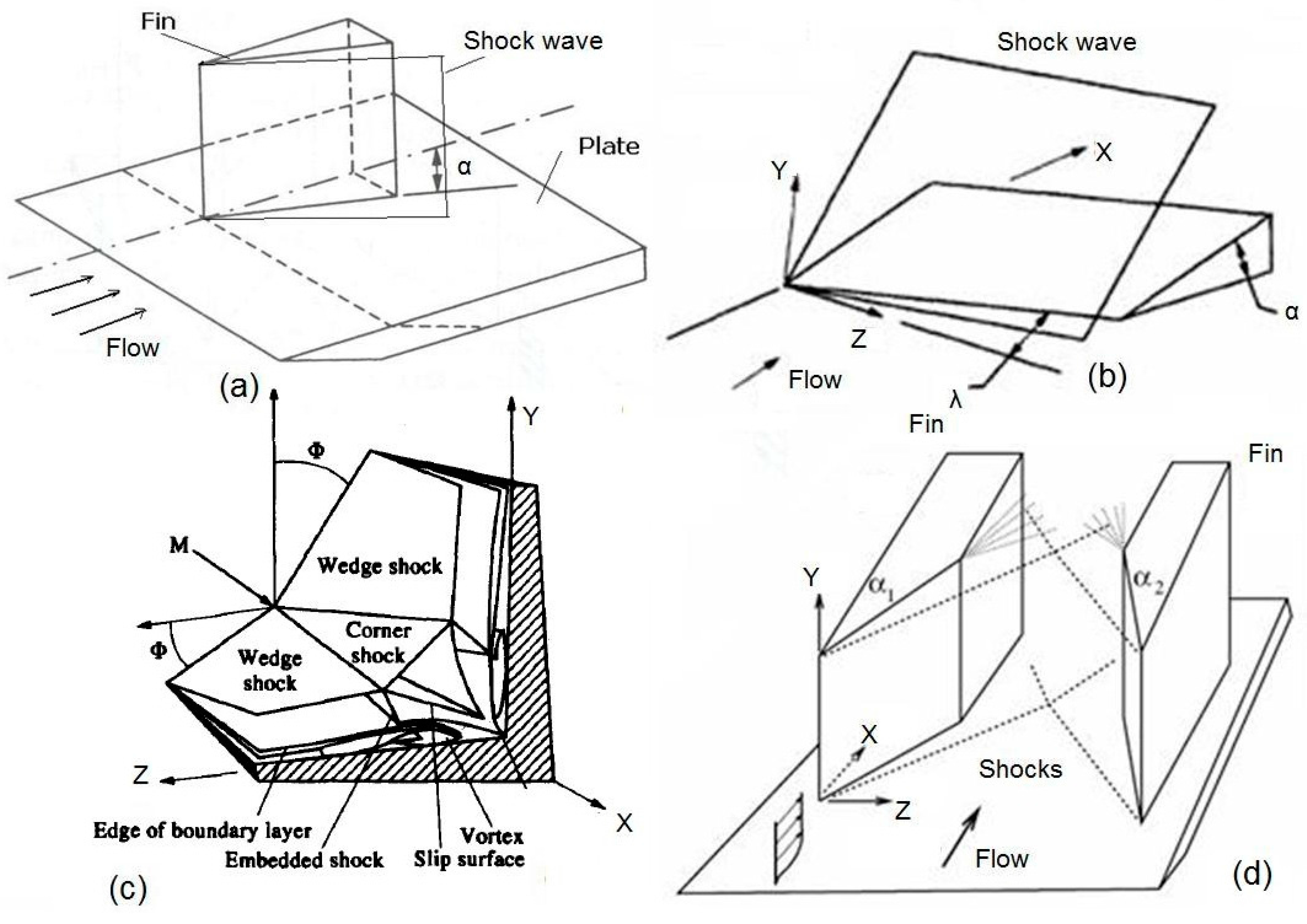
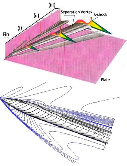
Object of the present study is the turbulence modeling of flows with extensive crossflow separation, i.e., three-dimensional flows in which the separated boundary layer rolls up into longitudinal vortices. This type of separation appears in many practical aerospace configurations; for example, subsonic/supersonic flow about slender bodies or delta wings at high incidence or in components of supersonic/hypersonic air vehicles when swept shock waves interact with boundary layers (Figure 1).

Figure 1. Formation of extensive crossflow separation: (a) Delta wing at high-incidence flow. Picture taken by H. Werle (ONERA) in a water-tank; (b) Swept shock/boundary layer interaction in a fin/plate configuration. The quasi-conical separation vortex is visualized by the contours of the eigenvalues of the velocity gradient field [1].

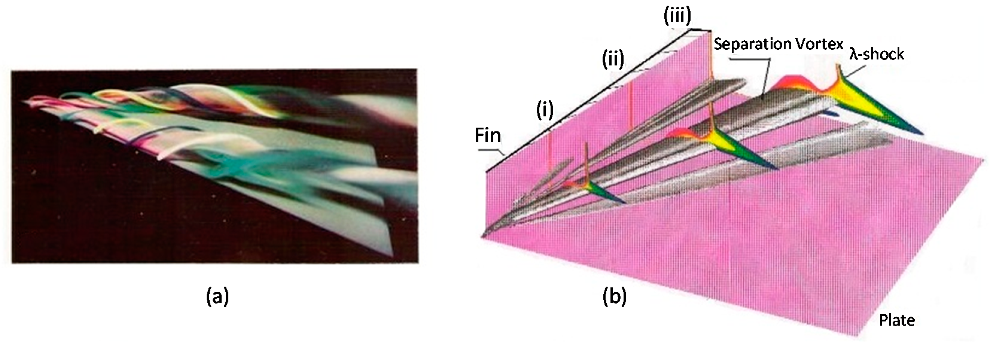
Figure 1. Formation of extensive crossflow separation: (a) Delta wing at high-incidence flow. Picture taken by H. Werle (ONERA) in a water-tank; (b) Swept shock/boundary layer interaction in a fin/plate configuration. The quasi-conical separation vortex is visualized by the contours of the eigenvalues of the velocity gradient field [1].

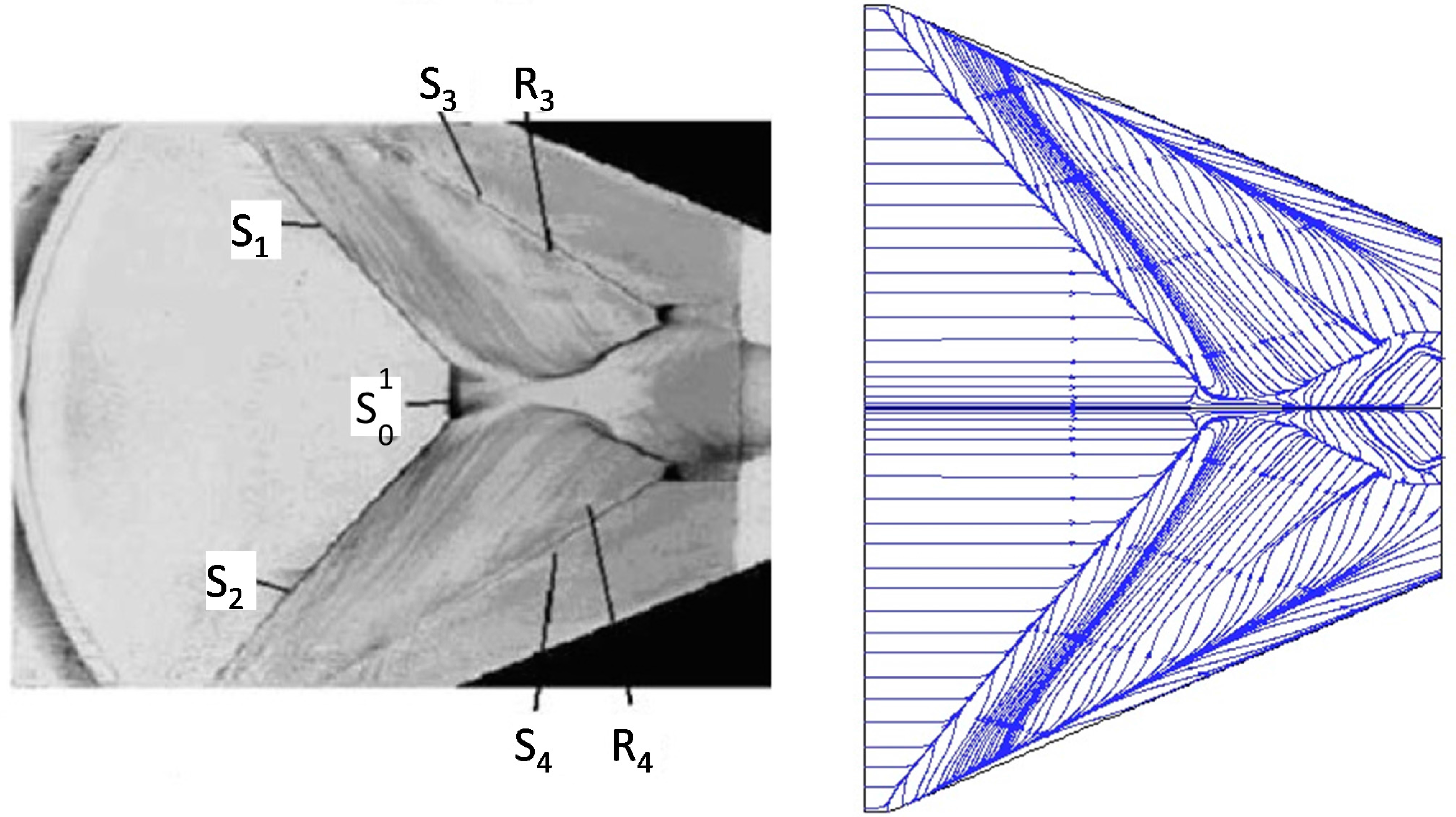
In the early 1950s, H. Werle of ONERA did pioneer work in visualizing high-angle of attack flows, like the delta wing shown in Figure 1a, by using a water tunnel and injecting colors from small holes at the expected regions of generation of the separation longitudinal vortices. The appearance of separation quasi-conical vortices of flattened shape in swept shock/boundary layer interactions, like that shown in Figure 1b for a fin/plate configuration, was hypothesized in the 1970s, but it was proved much later. Indeed, this early period oil-flow visualization revealed the existence on the surface of the plate, below the separation bubble, of a separation and an attachment line, which away from the apex of the configuration are straight and intersect upstream of the apex and close to it. The trace of the inviscid shock also passes through this intersection. It has been proposed that the separation bubble is actually a conical flat vortex. More than 20 years of experimental and computational research were required for proving these early hypotheses (see [2,3] for details).

Returning to turbulence modeling, it is mentioned that according to published evidence, the accuracy of prediction of flows with extensive crossflow separation is marginal. Particularly for shock wave/turbulent boundary layer interactions (SBLIs), Knight and Degrez [4] summarizing results of comparisons of several contributions (organized by Advisory Group for Aerospace Research and Development (AGARD)), using the RANS equations with a wide range of turbulence model from zero equations to full Reynolds Stress Equation formulations, state:

Simulation accuracy is good for mild interactions, marginal for strong ones. For wall heat transfer rate, the deviation of the calculated results from experiment ranges from 40% to 150%. Calculations predict “more turbulent” flows, compared to experiments.

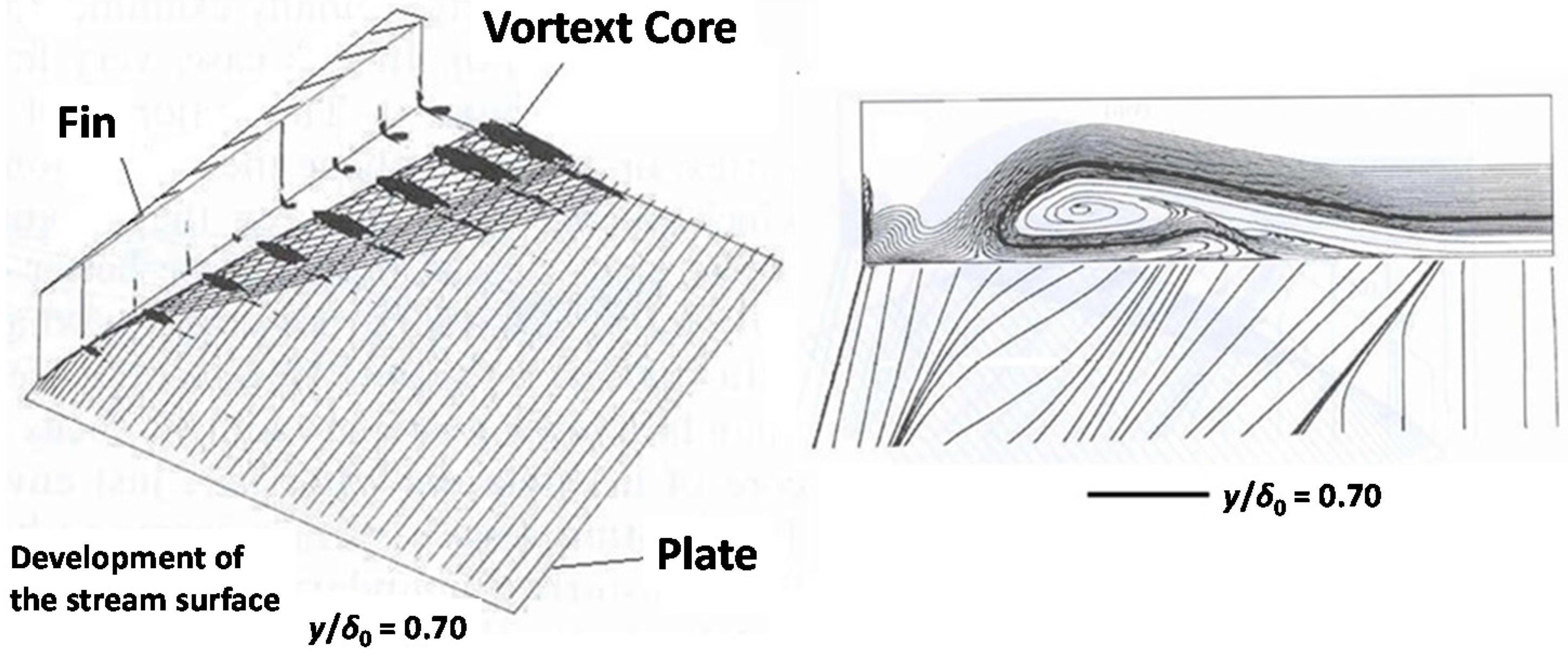
To explain this condition, the present author [5] studied the effect of the longitudinal separation vortices on the turbulence of the flow. It is reminded that a characteristic feature of vortices is their strong swirling motion, allowing them to promote large-scale mixing of fluids with possibly different momentum and energy. Panaras [5] hypothesized that the longitudinal vortices generated in the types of flows shown in Figure 1, transfer external inviscid air into the lower turbulent part of the separated flow, decreasing its turbulence. 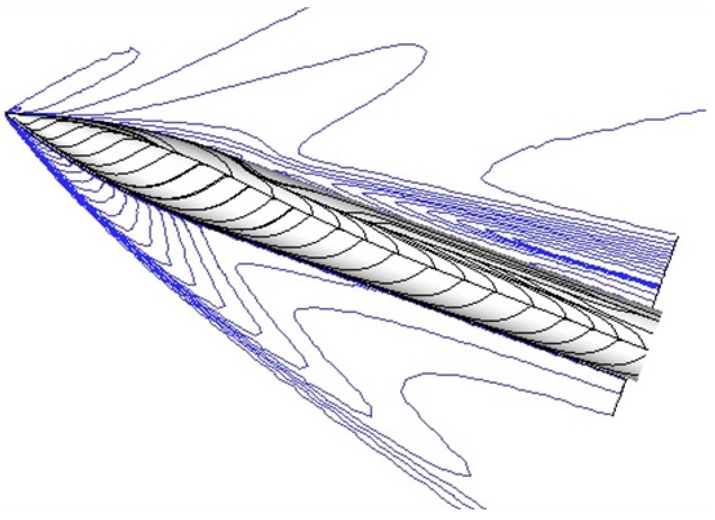To prove his hypothesis, Panaras [5] studied numerically the structure of the separation vortex, which appears in a strong swept shock wave/turbulent boundary layer interaction generated in a fin/plate configuration. He studied the flowfield by means of stream surfaces starting at the inflow plane within the undisturbed boundary layer, which is initially parallel to the plate. Each of these surfaces was represented by a number of streamlines. Calculation of the spatial evolution of selected stream surfaces revealed that the inner layers of the undisturbed boundary layer, where the eddy viscosity is high, wind around the core of the separation vortex. However, the outer layers, which have low turbulence, rotate over the separation vortex and penetrate into the separation bubble at the attachment region, forming a low-turbulence tongue, which lies along the plate, underneath the vortex (Figure 2). The intermittency of the fluid that constitutes the tongue is very small, that is, the flow is almost laminar there. At the initial stage of development, the conical separation vortex is completely composed of turbulent fluid, but as it grows linearly downstream the low-turbulence tongue is formed.

The analysis of Panaras [5] leads to the conclusion that laminarization of the initially turbulent flow appears in case of extensive crossflow separation. Hence, the Boussinesq equation is not adequate for the estimation of the Reynolds stresses. With reference to Figure 2, it is mentioned that although the mean strain is very high in the near wall reversed flow, the flow there is almost laminar. Evidently, application of Boussinesq’s equation in this region predicts higher Reynolds stresses than the actual ones. Related examples will be given in Section 3.1.

Figure 2. Structure of the separated flow in a swept-shock/turbulent boundary-layer interaction. Flow conditions: M_∞ = 4.0, α = 16° [5].

Figure 2. Structure of the separated flow in a swept-shock/turbulent boundary-layer interaction. Flow conditions: M_∞ = 4.0, α = 16° [5].

The discovery of the laminarization of the initially turbulent flow, in flows with extensive crossflow separation led to the development of new ideas in turbulence modeling for shock wave/turbulent boundary layer interactions (SBLIs). These new ideas include realizability (weak nonlinearity) and specific physical models, which incorporate known flowfield behavior [6,7]. In a short period the simulation accuracy of SBLIs was improved. This is clearly evident if the content of the critical survey of Computational Fluid Dynamics (CFD) prediction capabilities for SBLIs prepared by Knight and Degrez [4] and of the similar review of Knight et al. [3], which was published only five years later, are compared. In spite of the spectacular improvement shown by the new models, even presently, the predicted skin friction and heat transfer are marginally accurate in simulations of flows with extensive crossflow separation. The present review has been prepared in order to stimulate further research, now that LES methods enter the field. Published and new data will be presented for 3-D SBLIs and high-alpha flows. New evidence will be given regarding the almost-laminar nature of the near wall reverse flow in these types of flow, including data from the first publication of fin/plate simulation by using LES [8].

2. Description of Codes and Turbulence Models

The CFD code ISAAC, developed by Morrison [9], is used in this study. ISAAC is a second-order, upwind, finite-volume method where advection terms in the mean and turbulence equations are solved by using Roe’s approximate Riemann solver coupled with the MUSCL scheme. Viscous terms are calculated with a central difference approximation. Mean and turbulence equations are solved coupled by using an implicit spatially split, diagonalized approximate factorization solver. ISAAC has been developed to test a large range of turbulence models. Algebraic models, various k–ε and k–ω formulations, and Reynolds stress transport models are included in ISAAC.

In the present article, the examined flows are calculated with the k–ω turbulence model of Wilcox [10], the Explicit Algebraic Reynolds Stress Model (EASM) of Rumsey and Gatski [11] and a modification of the algebraic turbulence model of Baldwin and Lomax [12] done by the present author, in order to improve its accuracy in separated flows.

It is known that the functional form of the Navier–Stokes equations is the same for laminar and turbulent flows. In the latter case, however, time average has been applied to equations, since in turbulent flows, each flow or thermodynamic parameter has a mean value and a random turbulent fluctuation (for example: $u_i={\overline{u}}_i+u_i^{\prime }$). The time averaged flow equations are known as Reynolds Averaged Navier–Stokes (RANS) equations. In them, new apparent shear stresses, known as Reynolds stresses: ${\tau }_{ij}=(\overline{\rho u_i^{\prime }{u}_j^{\prime }})$, have appeared, which need to be calculated. The calculation of the Reynolds stresses is not easy; transport equation for each of them must be solved, increasing the total CPU cost. Alternatively, the Boussinesq hypothesis is applied, according to which the apparent turbulent shear stresses are related to the rate of mean strain, through an apparent scalar turbulent or “eddy” viscosity coefficient, μ_t. For the calculation of the turbulent viscosity coefficient, various turbulence models have been developed, in which the Reynolds stresses and other terms of turbulent fluctuation parameters are related to mean values of the flow: ${\overline{u}}_i,\overline{T},\overline{\rho }$. The Boussinesq equation is,

$$-\rho {\tau }_{ij}={\mu }_t(S_{ij}-\frac{1}{3}{S}_{kk}{\delta }_{ij})-\frac{2}{3}\rho k{\delta }_{ij}$$

(1)

where k is the turbulent kinetic energy and S_ij is the strain rate tensor given by,

$$S_{ij}=\frac{1}{2}(\frac{\partial {\overline{u}}_i}{\partial x_j}+\frac{\partial {\overline{u}}_j}{\partial x_i})$$

(2)

The k–ω turbulence model of Wilcox [10] is a linear eddy viscosity model, which includes Equation (1) in its formulation. The eddy viscosity, μ_t, is related to mean and turbulent quantities by,

$${\mu }_t=C_{\mu }\frac{\rho k}{\omega }$$

(3)

where ω is the specific dissipation rate.

The turbulent kinetic energy and specific dissipation rate are calculated by solving transport equations similar to those that express the flow parameters (see [10]).

The explicit algebraic stress model (EASM) of Rumsey and Gatski [11] replaces the linear Boussinesq approximation with a non-linear relationship of the strain rate and rotation rate tensors,

$$-\rho {\tau }_{ij}={\mu }_t^{*}f(S_{ij},W_{ij},k)$$

(4)

where W_ij is the rotation rate tensor,

$$W_{ij}=\frac{1}{2}(\frac{\partial {\overline{u}}_i}{\partial x_j}-\frac{\partial {\overline{u}}_j}{\partial x_i})$$

(5)

The eddy viscosity is given by,

$${\mu }_t^{*}=-\rho k{\alpha }_1$$

(6)

and α₁ is obtained by a solution of a cubic equation. The non-linear relation of Rumsey and Gatski [11] is coupled with the regular k–ω equations of Wilcox [10].

The Baldwin–Lomax [12] model is a two-layer algebraic zero-equation model. The eddy viscosity coefficient is given by algebraic equations. In the inner layer it follows the Prandlt–Van Driest formulation:

$${({\mu }_t)}_{inner}~{\eta }^2\Omega$$

(7)

where Ω is the absolute value of the vorticity and η is the distance normal to the wall.

In the outer layer the following equations are used:

$${({\mu }_t)}_{outer}~F_{wake}$$

(8)

$$F_1={\eta }_{max}{F}_{max}$$

(9)

$$F_2=\frac{c_{wk}{\eta }_{max}{u}_{dif}^2}{F_{max}}$$

(10)

$$F_{wake}=\min \left(F_{\mathit{1}},F_{\mathit{2}}\right)$$

(11)

The quantity F_max is the maximum value of the moment of vorticity:

F(η) = ηΩD

(12)

The parameter η_max is the value of η at which F(η), Equation (12), is maximum. D is the van Driest damping factor (see [12]).

The quantity u_dif is the difference between maximum and minimum velocity in the velocity profile. The thickness of the boundary layer is defined by: δ = η_max/C_kleb. The constants appearing in the previous relations are: C_wk = 0.25, C_Kleb = 0.3.

The present author [7] considered the discovered laminarization of the flow for the derivation of a new equation for the calculation of the eddy-viscosity coefficient in the region of a separation vortex. He followed the Baldwin–Lomax turbulence model. According to his equation, in regions of high transverse velocity gradients the predicted value of μ_t is smaller than the value predicted by the regular equations of the Baldwin–Lomax model. The developed model was tested both in high-angle of attack flows and shock wave turbulent boundary layer interactions (Panaras [7,13]). The agreement with the experimental evidence was very good. In its initial form, the Panaras modeling is difficult to use, since it requires a preliminary run, so that the user will define “reference conditions” for the wake function of the Baldwin–Lomax model. Also, the prediction of the line of separation for the application of the new relation is required. In this paper, a new version is presented, in which the Baldwin–Lomax model keeps its original formulation, but one of the basic equations for the estimation of the turbulent viscosity coefficient is changed, to follow the structure of turbulent separated flows. More particularly, the η_max in Equation (10) is replaced by a reference value, η_ref. The value of η_ref differs from flow to flow and it is based on existing semi-empirical relations that define the boundary layer parameters of an equivalent flat plate flow of the same Reynolds number.

For the estimation of η_ref along a flat-plate flow, the semi-empirical analysis of Falkner [14] is used, which is valid for a Reynolds number between 10⁵ and 10¹⁰. According to Falkner [14], the boundary layer growth along a flat plate is,

$$\delta =\frac{0.1285x}{R{e}_x^{1/7}}$$

(13)

If this equation is combined with the relation: δ = η_max/C_Kleb, then,

$$\frac{{\eta }_{\max }}{x}=\frac{0.1285\times C_{Kleb}}{R{e}_x^{1/7}}=\frac{0.03855}{R{e}_x^{1/7}}$$

(14)

Defining η_ref at a characteristic separation length of each examined configuration, L_sep, the final calculation scheme is,

$${\eta }_{ref}=\frac{L_{sep}}{L}\frac{0.03855}{R{e}_{L_{sep}}^{1/7}}$$

(15)

where η_ref has been non-dimensionalized by the length of the body, L.

Then Equation (10) is replaced by,

$$F_{\mathit{2}}=\frac{c_{wk}{\eta }_{ref}{u}_{dif}^2}{F_{max}}$$

(16)

For aerospace configurations we propose the equality: L_sep = L. But if there is extensive crossflow separation, as in the case of slender bodies at incidence, more accurate results are obtained if the characteristic length is equal to a crossflow length (L_sep = d, for axisymmetric bodies). This assumption is reasonable, since in high-alpha flows, the flowfield is dominated by the separated crossflow.

3. Results

3.1. Swept-Shock Boundary Layer Interactions

Swept-shock boundary layer interactions occur in the axial supersonic or hypersonic flow between two intersecting surfaces, for example in junctions between wing/body and fin/body, intake ducts of engines, as well as in the transonic flow over a sweptback wing. Many investigations of the phenomenon, both experimentally and computationally more recently, have been undertaken in the last 50 years. Most of these research studies involved configurations that are simplified shapes of various elements of high-speed vehicles. The configurations can be classified as having either one or two surfaces producing a compression in the flow field. The simplest example of the former type of configuration consists of a sharp fin (or wedge) attached normally to a flat plate at a certain distance behind its leading edge as shown in Figure 3a. The swept compression corner is another simple example (Figure 3b). The corner formed by the intersection of two wedges (Figure 3c) is the basic configuration of flows with two surfaces providing compression. This configuration is usually called an axial corner. Relatively recently, interest has been shown in an extension of the single fin geometry, consisting of two fins or wedges attached normally to a flat plate (Figure 4d). This is called a crossing shock configuration.

If the aforementioned interactions are strong, undesirable effects can be present such as local high heat transfer rates and static pressures. In both types of interactions, with one or with two compression surfaces, the conditions close to the surface are similar: the oblique shock wave generated at the compression surface, intersects the boundary layer on the plate and an interaction field is generated. Thus, we would expect that the major features of the viscous–inviscid interaction part of the flow field are the same in both configurations. As regards the flow conditions emphasis has been given to supersonic speeds and turbulent boundary layers in the fin/plate configuration. Although there are early experimental results on flows with turbulent supersonic conditions in the case of the axial corner, the majority of the studies are related to laminar hypersonic flows. A general overview of the structure of the flows in the configurations shown in Figure 3 is given by Panaras [2]. In a more recent review, Knight et al. [3] concentrate on the CFD prediction capability of the flow in single and double fin/plate configurations.

Figure 3. Generic configurations of SBLI used for experimental and computational studies.

Figure 3. Generic configurations of SBLI used for experimental and computational studies.

Figure 4. Wall pressure and skin friction variation: (a,b) SF4 test case and (c,d) SF6 test case [13].

Figure 4. Wall pressure and skin friction variation: (a,b) SF4 test case and (c,d) SF6 test case [13].

3.1.1. Fin/Plate Configuration

As regards the fin/plate configuration, data from the critical survey of Knight and Degrez [4] are presented in Figure 4. The flow conditions for the SF4 test case are: M_∞ = 4.0, α = 16°, Re_δo = 2.1 × 10⁵. The test case SF6 differs in the fin angle (α) relative to the freestream (stronger interaction): M_∞ = 4.0, α = 20°, Re_δo = 2.1 × 10⁵. These two test cases were simulated by various contributors using the baseline Baldwin–Lomax, Panaras [7] B–L modification, k–ε and Spalart–Allmaras–Edwards turbulence models. The surface pressure along an arc across the flowfield is shown in Figure 4a,c. According to Knight and Degrez [4]:

The Baldwin–Lomax–Panaras and Spalart–Allmaras–Edwards models are the most accurate. Both models predict the surface pressure in the plateau region within 5% to 10%. Also, both models display a pressure trough at the region of appearance of secondary separation, in agreement with the experiment. Both models overestimate the peak pressure in the vicinity of the corner. The predictions of the Baldwin–Lomax and k–ε models exhibit the general trends of the experiment but are less accurate.

The skin friction coefficient is displayed in Figure 4b,d.

In the stronger interaction (Figure 4d) the Baldwin–Lomax–Panaras and Spalart–Allmaras–Edwards models predict a peak in the vicinity of the corner which is not evident in the experiment; in particular, their computed values at the experimental location β = 26.5° are substantially above the experiment. Additional measurements in the region 22° < β < 26° would be helpful in determining whether a peak appears. Elsewhere, all four models provide generally good agreement with the experiment.

It is reminded that the Spalart–Allmaras turbulence model solves a modeled transport equation for the kinematic eddy viscosity. The model was designed specifically for aerospace applications involving wall-bounded flows and has been shown to give good results for boundary layers subjected to adverse pressure gradients. Edwards and Chandra [15] developed a form, which improves the near-wall numerical behavior of the model (i.e., the goal was to improve the convergence behavior).

The success of the modified Baldwin–Lomax model [7] to describe rather accurately 3-D SBLIs motivated Thivet et al. [6] to construct a weakly nonlinear version of the k–ω model. More particularly, they implemented into the k–ω model an extension to compressible flows of the nonlinear correction of Durbin [16]. Application of this modification to a very strong sharp fin/plate flow (M_∞ = 4, α = 30.6°, Re_δo = 1.6 × 10⁵) resulted in a remarkably accurate simulation. Herein, we present in Figure 5 the results of Thivet et al. [6], as they have been given by Zheltovodov [17], who is co-author of the basic paper and provided the experimental data. As seen in Figure 5b, the nonlinear model (WI-DU, line 4) shows a significant improvement relative to the linear k–ω model (line 3) and standard Baldwin–Lomax model (B–L, line 2) and correctly predicts wall pressure distribution as well as secondary separation phenomena in a vicinity of the local normal shock wave in the supersonic turbulent cross near-wall “reversed” flow (Figure 5a). Also, in contrast to other standard turbulence models (B–L, k–ω, k–ε), the weakly nonlinear model of Thivet et al. [6] predicts well the wall skin friction in the interaction region (see [6]).

Figure 5. Single fin flow at α = 30.6°, M_∞ = 4, Re_δo = 1.6 × 10⁵: (a) flowfield schematic in a cross section and (b) wall pressure distribution. Reprinted [17] by permission from the author.

Figure 5. Single fin flow at α = 30.6°, M_∞ = 4, Re_δo = 1.6 × 10⁵: (a) flowfield schematic in a cross section and (b) wall pressure distribution. Reprinted [17] by permission from the author.

With the kind permission of the authors, we present data from the first ever to be performed Large Eddy Simulation of hypersonic SBLI around a fin/plate configuration (Fang et al. [8]). The flow data were: M_∞ = 5, α = 30.6°, Re_o = 37.0 × 10⁶/m). The performed LES has demonstrated very good agreement with available experimental data in terms of the mean flowfield structure, the surface pressure, as well as the surface flow pattern. However, significant under-prediction in the surface skin-friction peak in the vicinity of the attachment line was observed. According to Fang et al. [8], the reasons of disagreement will be investigated. The wall pressure distribution is shown in Figure 6. The good agreement with the experimental data is evident. In Section 4, flowfield data from this LES study will be presented, which support and enforce the observation, done earlier by Panaras [5], for the laminarization of the initially turbulent flow by the induction mechanism of the separation vortex.

Figure 6. LES of fin/plate configuration. Comparison of wall pressure distribution. Reprinted [8] by permission from the authors.

Figure 6. LES of fin/plate configuration. Comparison of wall pressure distribution. Reprinted [8] by permission from the authors.

3.1.2. Crossing Shock Interaction

The nonlinear k–ω model of Thivet et al. [6] and the algebraic model of Panaras [7], which both were developed considering the structure of the separated flow, predict with sufficient accuracy the flow structure and wall pressure distribution of crossing shock configurations. Related results are included in the survey of Knight et al. [3]. In the present, in order to check the accuracy of the proposed algebraic turbulence model (Section 2), the very strong 23° × 23° crossing shock interaction studied by Schuelein and Zheltovodov [18] in the supersonic/hypersonic Ludwieg tube of DLR/Goettingen, at M_∞ = 5.0 is examined. The two fins are symmetric (Figure 7). The stagnation conditions were P₀ = 2.2 MPa and T₀ = 427 K, resulting in a freestream unit Reynolds number of 36.5 × 10⁶/m. The incoming boundary layer was an equilibrium turbulent boundary layer with an isothermal wall (T_w = 295 K). The boundary and momentum thicknesses were δ₀ = 3.8 mm and θ = 0.157 mm at a distance of 6δ₀ upstream of the fin leading edge. A Navier–Stokes solver based on an upwind total variation diminishing (TVD) scheme and developed by A. Panaras and B. Mueller at DLR is used. The baseline and the modified B–L models are tested. For the application of the turbulence model, the existence of two intersecting surfaces dictates the use of a “modified distance”, originally proposed by Hung and MacCormack [19] to account for the turbulent mixing length near the intersection of the surfaces. The DLR upwind code incorporates this feature. For this reason this code is used, instead of ISAAC.

Figure 7. Simulated crossing shock configuration.

Figure 7. Simulated crossing shock configuration.

Due to the simplicity of the configuration geometry, the mesh was generated algebraically. Clustering was applied close to the plate and to the fin for adequate resolution of the viscous effects. For both configurations, at each crossflow plane 91 × 101 points (z-, y-directions) are used. In the streamwise x-direction there are 117 grid planes uniformly. The inflow plane is located at a distance equal to 2δ₀ upstream of the leading edge of the fins. The height of the computational field is 26.8δ₀. For the simulation of the undisturbed boundary layer, 45 points are used.

The walls are assumed impermeable and no-slip boundary conditions are applied. The boundary layer profile upstream of the interaction region is used as boundary condition on the inflow plane and as initial condition for the whole flow field. This profile was calculated by a 2-D procedure, from the leading edge of the flat plate to the leading edge of the fin. Symmetry condition was applied along the centerline of the plane (the velocity component which is normal to the symmetry plane is assumed equal to zero). The gradients of the flow parameters are set equal to zero on the upper and outflow far field boundaries. The temperature of the walls is assumed constant (isothermal condition) with T_wall/T_adiabatic = 4.15.

The 23° × 23° experimental oil-flow visualization is compared with the computed surface streamlines in Figure 8. It is observed in this figure that the computation reproduces accurately the topological features shown in the experiment. Superposition of the results has shown that the separation lines coincide, while the computed secondary separation lines are very close to the experimental ones.

Figure 8. Comparison of surface streamlines with experimental oil-flow lines.

Figure 8. Comparison of surface streamlines with experimental oil-flow lines.

Schuelein and Zheltovodov [18] have measured the wall pressure distribution at various cross sections. The experimental and the computed crossflow wall pressure distributions are compared in Figure 9. The distance (x) is measured from the leading edge of fins; also the origin of the z-axis corresponds to the centerline of the configuration. It is seen in this figure that the results that are based on the modified B–L model agree very well with the experimental evidence. In most of the stations, the predictions and the experimental data coincide. A small disagreement is observed in the region close to the centerline at station x = 124 mm, just downstream of the intersection of the primary separation lines. The same behavior is observed in the accurate simulation of this flow by Schmisseur and Gaitonde [20] using the k–ε model with low Reynolds number and compressibility correction (Figure 10).

Figure 9. Surface pressure distribution comparison at various cross sections.

Figure 9. Surface pressure distribution comparison at various cross sections.

Figure 10. Wall pressure prediction of Schmisseur and Gaitonde [20].

Figure 10. Wall pressure prediction of Schmisseur and Gaitonde [20].

3.2. Supersonic Ogive Cylinder

An experimental study of the flow around a 3-caliber tangent ogive-cylinder body in a supersonic flow was conducted at ONERA with the aim of constituting an experimental database for code validations (Barberis [21]). Results were obtained for natural and fixed transition. The test conditions were: M = 2.0, Re_L = 1.44 × 10⁶ and incidence α = 10° to 20°. The measurements included surface-pressure distributions at various cross-sections. For natural transition, the authors used acenaphtene coating visualization to verify that the boundary layer remained laminar over the entire body at α = 0 degree. Transition was triggered by means of a 5 mm wide carborundum strip located at x/d = 1.0, where d is the diameter of the body.

This test case is included in the turbulence model validation study of Morrison et al. [22]. In the present paper, the turbulent α = 20° flow is simulated by using the ISAAC code. Morrison et al. [22] used three half-body grids. The finest of them consists of 99 points in the streamwise directions, 101 points circumferentially and 115 points normal to the wall (99 × 101 × 115). In addition to that, a finer one (184 × 121 × 115) was used in the present work. Laminar flow was assumed from the tip of the body to the station x/d = 1.0. Downstream of this point, the algebraic, the k–ω and the EASM turbulence models were applied.

Figure 11 shows the side view of the surface streamlines and the density contours at the symmetry plane, calculated with the modified B–L model. The calculated wall pressure distribution along the circumferential direction, φ, is compared to the experimental data at four axial stations in Figure 12. The agreement with the experimental values is very good, except near φ = 80°, where the flow separates. The modified B–L model and the k–ω model predict a smaller separation occurring later than the experimental data show. The EASM model of Rumsey and Gatski [11] consistently predicts an earlier separation with a larger vortical flow region than the other models, and it is in closer agreement with the experimental data. On the leaward side, the modified B–L and the EASM models are closer to the experimental evidence than the k–ω model.

Figure 11. Surface streamlines and density contours for ogive cylinder in supersonic flow.

Figure 11. Surface streamlines and density contours for ogive cylinder in supersonic flow.

Regarding the effectiveness of the carborundum strip to trigger transition, Barberis [21] mentions that it has been verified by using the acenaphtene technique that transition occurred at the location of the carborundum strip for all incidences. However, since the Reynolds number is relatively small and because of the appearance of crossflow, the artificially triggered transition is probably not adequate to establish turbulent flow along the whole body. The α = 10° test case has been clarified by van den Weide and Deconinck [23], who have simulated both the laminar and turbulent flow. According to them, the laminar computation turned out to be at the limit of unsteadiness, suggesting that the test conditions are transitional in reality. The turbulent computation was steady and the results for the pressure distribution compared well with the experimental data obtained at ONERA. Significant differences between the laminar and turbulent computation were found in the vortex pattern developing on the leaward side. In the case of α = 20°, the experiments do not indicate significant differences in the vortex pattern developing on the leaward side, between the natural and triggered transition tests (see inset in Figure 14). In addition, since the crossflow is more extensive, it is probable that the carborundum strip was not sufficient to establish turbulent flow along the whole body. To test this hypothesis, laminar calculations were performed for the α = 20° test case. The results are shown in Figure 13 and indicate that they are closer to the experiments than the turbulent simulations, especially regarding the position of separation of the flow. On the leaward side, the agreement is better at stations x/d = 7.5 and 8.5. In view of these results, a numerical test was performed, in which the turbulent simulations were repeated by assuming that the Reynolds number is based on the diameter of the body (dividing the actual Reynolds number by 9, Re_d = 1.6 × 10⁵). These results are also shown in Figure 13 and indicate that this prediction is much closer to the data, than the regular results shown in Figure 12. As regards the turbulence structure of the two solutions, the distribution of turbulent kinetic energy (TKE) is shown in Figure 14 at the cross-sections x/d = 4.95 and 8.5, for the calculations employing the EASM model. In this figure, it is evident that in the solution based on Re_d, the flow is practically laminar within the separation bubble.

Figure 12. Ogive-cylinder: comparison of wall pressure coefficient at various cross sections. Reynolds number based on body length.

Figure 12. Ogive-cylinder: comparison of wall pressure coefficient at various cross sections. Reynolds number based on body length.

Figure 13. Ogive-cylinder: comparison of wall pressure coefficient at various cross sections. Reynolds number based on diameter.

Figure 13. Ogive-cylinder: comparison of wall pressure coefficient at various cross sections. Reynolds number based on diameter.

Figure 14. EASM calculations: Turbulent kinetic energy (TKE) distribution in two cross-sections. Calculations using Reynolds number based on length or diameter of body. Inset: experiment, flow visualization by total pressure at cross-section x/d = 4.95 [21].

Figure 14. EASM calculations: Turbulent kinetic energy (TKE) distribution in two cross-sections. Calculations using Reynolds number based on length or diameter of body. Inset: experiment, flow visualization by total pressure at cross-section x/d = 4.95 [21].

4. Further Evidence of Laminarization of the Separated Flow in 3-D SBLIs

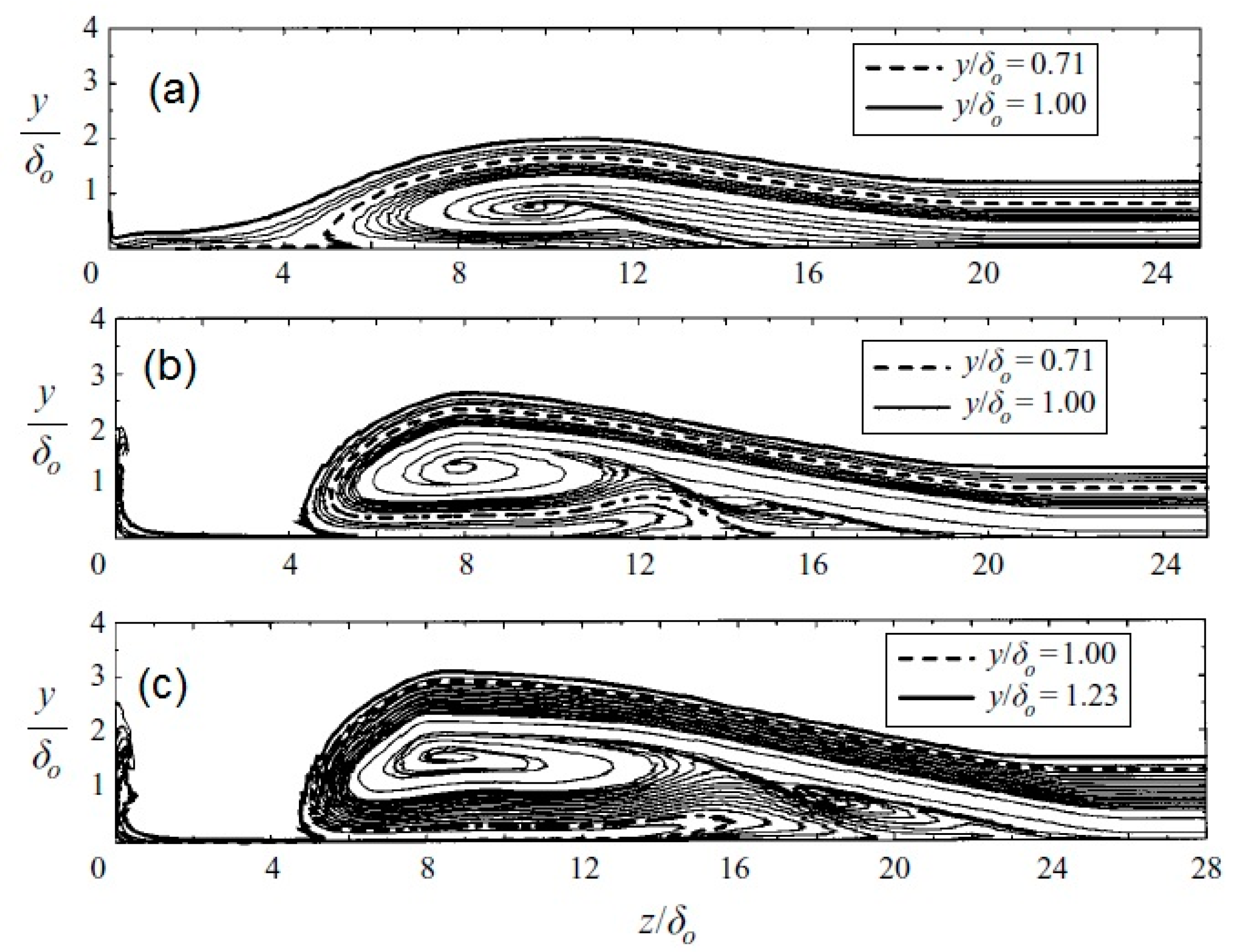
To return to the theoretical analysis, we note that in the basic article of Panaras [5], the effect of the strength of the interaction on the laminarization of the separation domain has been addressed. By studying various test cases of fin/plate flows, Panaras [5] found that increase in the strength of the interaction results in the folding of higher inviscid layers around the vortex. In the other extreme of a weak interaction, no low-turbulence tongue is formed. Crossflow cuts of three studied flows are shown in Figure 15. The cuts correspond to station (iii) of Figure 1b and they have been arranged according to the interaction strength. The first cut belongs to a weak interaction, M_∞ = 3.0, α = 10°. In Figure 15a, it is seen that qualitatively this flow develops as described in Section 1. A primary vortex is formed, around which a part of the separated boundary layer folds and penetrates into the separation region. However, the vortex is very weak (its spiral core is small), and the layer folded around originates from the inner part of the boundary layer and not from the outer one. Hence, there is no formation of a low-turbulence tongue. Observation of the surface skin-friction lines (not included here) has indicated that no secondary vortex appears. In the test case shown in Figure 15b (M_∞ = 4.0, α = 16°), the y/δ₀ = 0.7 stream surface envelops the secondary vortex and a low turbulence tongue is formed. Also, the stream surface y/δ₀ = 1.0 folds around the vortex. At the other extreme is the flow examined in Figure 15c. This interaction is generated in a M_∞ = 4.0, α = 20° fin/plate flow, and the stream surface y/δ₀ = 1.0 penetrates deeply into the separation region and it is, actually, a part of the secondary vortex. Furthermore, the layers of the tongue adjacent to the plate (under the primary vortex) are practically laminar, because they are composed of air that originates outside the boundary layer (between y/δ₀ = 1.0 and 1.23).

Figure 15. Cross-sections of various flows: (a) M_∞ = 3.0, α = 10°; (b) M_∞ = 4.0, α = 16°; and (c) M_∞ = 4.0, α = 20° [5].

Figure 15. Cross-sections of various flows: (a) M_∞ = 3.0, α = 10°; (b) M_∞ = 4.0, α = 16°; and (c) M_∞ = 4.0, α = 20° [5].

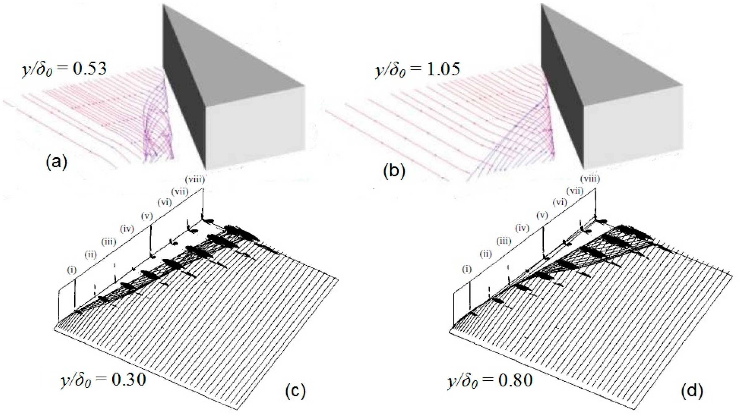
The spatial evolution of a selected number of stream surfaces originating within the upstream boundary layer and initially parallel to the plate, has also been examined by Fang et al. [8] in their very recent LES calculations. Results from their simulated very strong interaction (M_∞ = 5, α = 30.6°) are compared in Figure 16 with the milder interaction results (M_∞ = 4.0, α = 16°) examined by Panaras [5]. Fang et al. [8] observe that the streamlines originating from the near-wall region (Figure 16a, y/δ₀ = 0.53) fold around the separation vortex core. With the increase of the origin position (Figure 16b, y/δ₀ = 1.05), the streamlines may directly enter the reversed flow, rather than through the vortex core. Equivalent conditions from the simulation of Panaras [5] are shown in Figure 16c,d. The data of Fang et al. [8], shown in figure 16, support the observation of Panaras [5] that in strong 3-D SBLIs the upper, less turbulent, part of the interacting boundary layer folds around the separation vortex and forms the reversed flow. Furthermore, Fang et al. 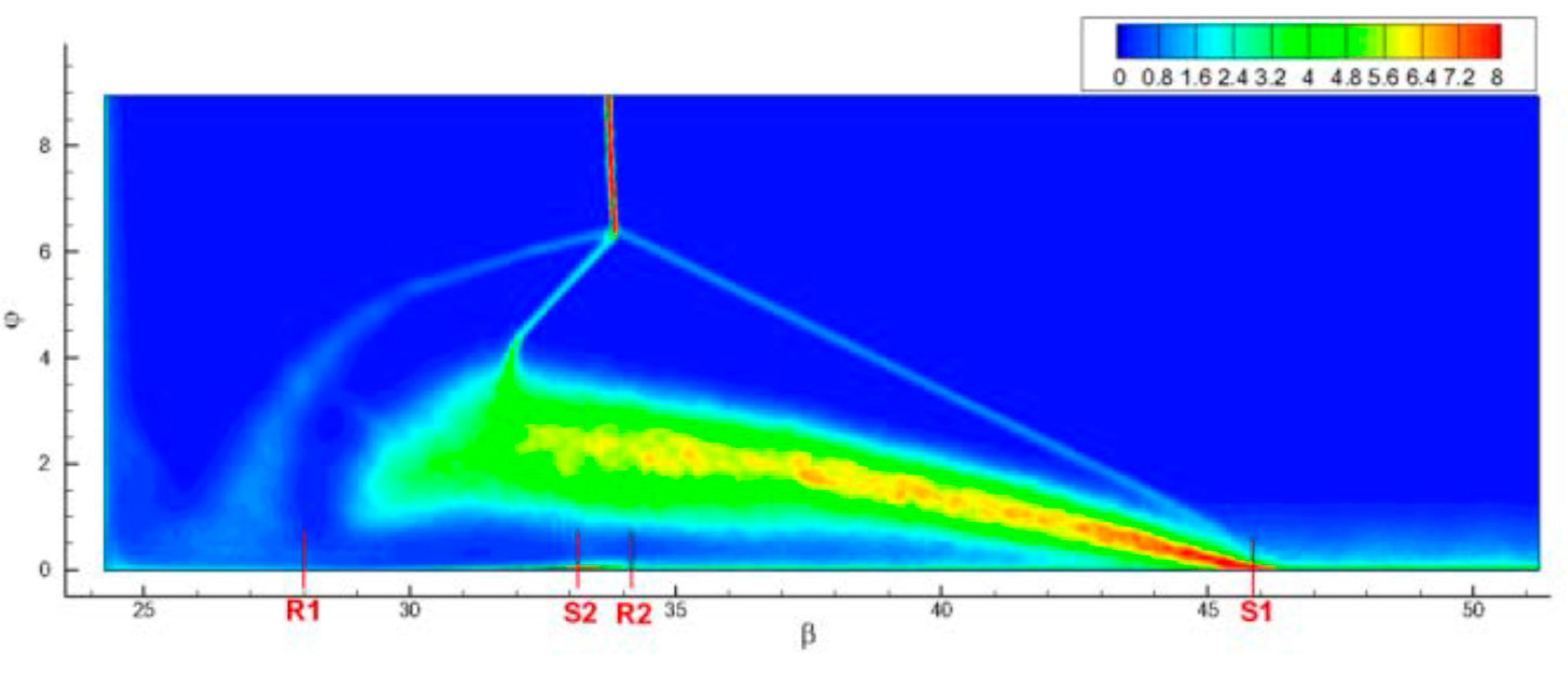[8] present the turbulent kinetic energy (TKE) distribution on a spherical section of the studied flowfield, close to the exit plane. Their data are reproduced here in Figure 17. In this figure, it is clear that the air, which folds around the separation vortex and forms its lower part near the wall, has very low turbulent kinetic energy, exactly as the analysis of Panaras [5] predicts. Amplification of turbulence is observed only in the near wall region downstream of the secondary separation (S₂), caused by the adverse pressure gradient existing in the region of S₂. The accurate LES calculations of Fang et al. [8] prove the hypothesis of laminarization of an originally turbulent flow in a swept shock/turbulent boundary layer interaction. We hope that Fang et al. [8] will include the distribution of TKE in more spherical sections in a future publication, so that the gradual laminarization along the separation vortex will be shown.

Figure 16. Development of stream surfaces originating at the inflow plate, at constant distance from the flat plate: (a,b) Data of Fang et al. [8]; (c,d) Data of Panaras [5].

Figure 16. Development of stream surfaces originating at the inflow plate, at constant distance from the flat plate: (a,b) Data of Fang et al. [8]; (c,d) Data of Panaras [5].

Figure 17. Turbulent kinetic energy (TKE) on the section at R = 226.3 mm, normalized with the square of the wall friction velocity at the inlet. Reprinted [8] with permission from the authors.

Figure 17. Turbulent kinetic energy (TKE) on the section at R = 226.3 mm, normalized with the square of the wall friction velocity at the inlet. Reprinted [8] with permission from the authors.

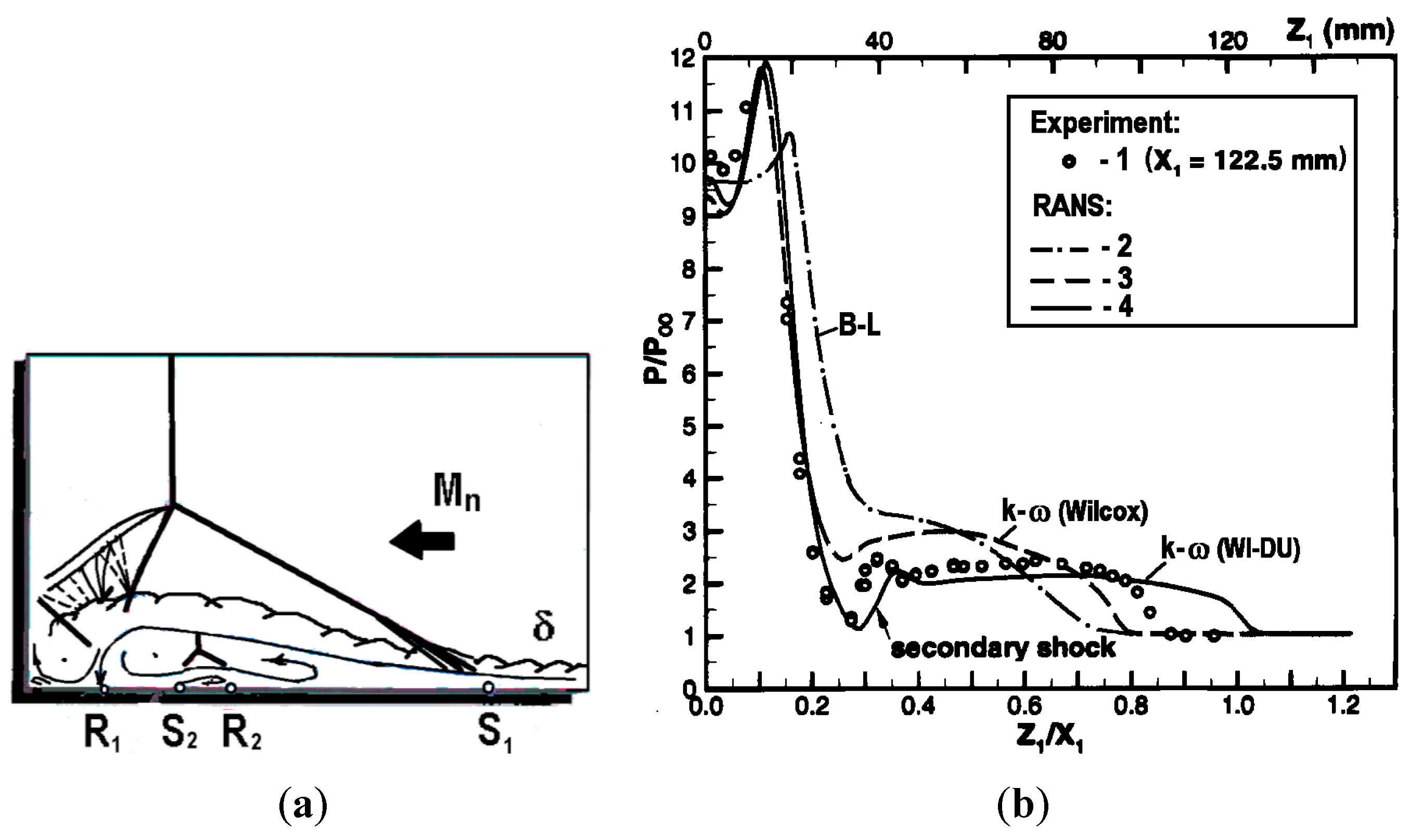
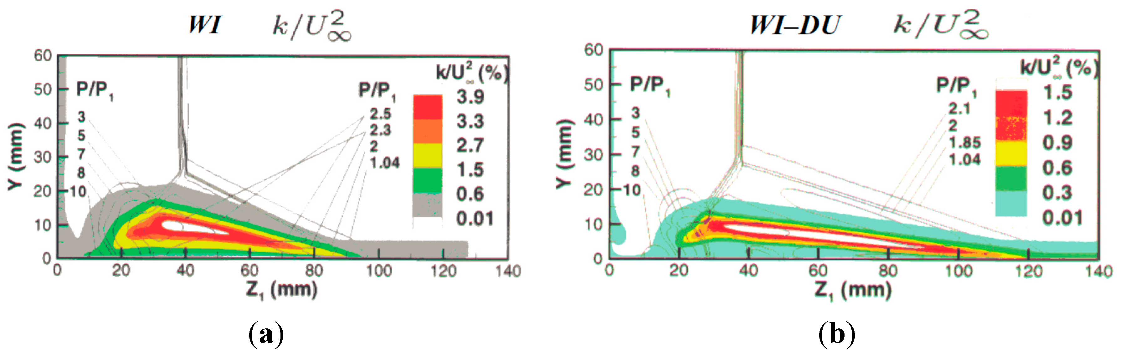
Finally, indirect evidence of laminarization of the separated flow in 3-D SBLIs is given by Zheltovodov [17], who commenting on the success of the weakly nonlinear model of Thivet et al. [6] to simulate accurately this class of flows, mentions that:

Such improvement is associated with significant reduction in the peak of turbulent kinetic energy in the flow which penetrates from an external part of the shear layer to the wall in the place of formation of the secondary separation line (Figure 18b) in contrast to the calculations with a standard k–ω model (WI, Figure 18a), which are characterized by high turbulence level in the near wall “reverse” flow”.

Figure 18. Turbulent kinetic energy in cross section (x₁ = 122.5 mm): (a) The linear Wilcox’s k–ω-model (WI); (b) Weakly nonlinear k–ω-model (WI–DU). Reprinted [17] by permission from the authors.

Figure 18. Turbulent kinetic energy in cross section (x₁ = 122.5 mm): (a) The linear Wilcox’s k–ω-model (WI); (b) Weakly nonlinear k–ω-model (WI–DU). Reprinted [17] by permission from the authors.

5. Conclusions

The reasons for the difficulty in simulating accurately with classical turbulence models strong 3-D SBLIs and high-alpha flows, which are characterized by the appearance of strong crossflow separation, are investigated. In view of recent additional evidence, an earlier flow analysis [5], which attributes the poor performance of classical turbulence models to the observed laminarization of the separation domain, is examined. According to this analysis, the longitudinal vortices into which the separated boundary layer rolls up, in this type of flow, transfer external inviscid air into the adjacent to the wall part of the separation, decreasing its turbulence. Increase in the strength of the interaction results in the folding of higher inviscid layers around the vortex. In the other extreme of a weak interaction, there is no laminarization. Strong evidence of laminarization of the flow in a very strong fin/plate SBLI is given in a recent LES simulation, by means of the predicted small value of the turbulent kinetic energy within the reverse flow in cross sections of the flow.

Existing linear turbulence models for closing the RANS equations relate the apparent turbulent shear stresses linearly to the rate of mean strain (Boussinesq’s equation). However, in the types of flows examined in the present article, although the mean strain is very high in the near wall reversed flow, the flow there is almost laminar. Evidently, application of Boussinesq’s equation in this region predicts higher Reynolds stresses than the actual ones. Published and new CFD results are presented which indicate that the accuracy of linear turbulence models is moderate in strong 3-D SBLIs. On the contrary, two-equation non-linear models and algebraic models that incorporate the previously described flowfield behavior, provide accurate results, regarding the flow structure, the wall pressure and skin friction distribution.

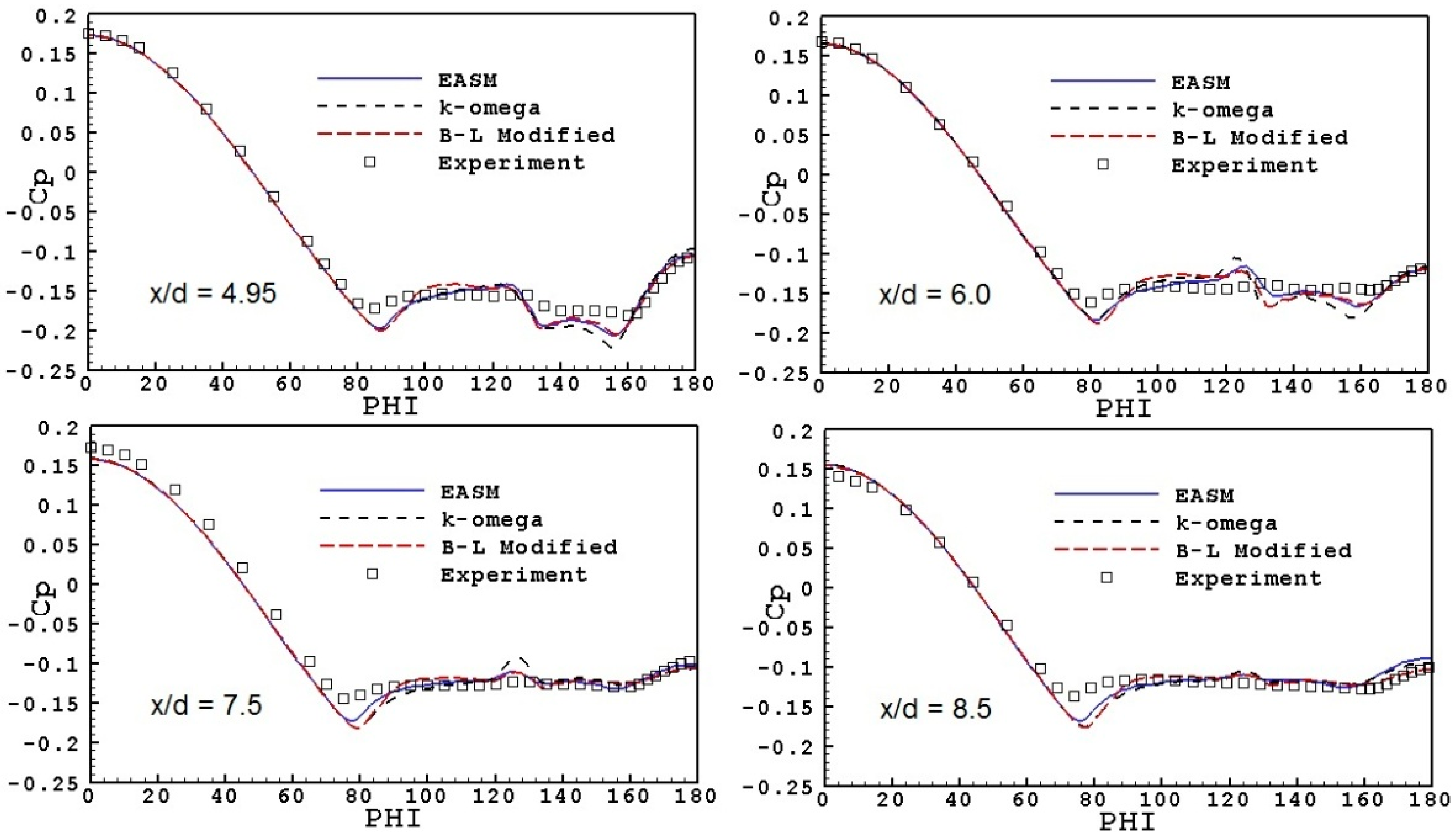
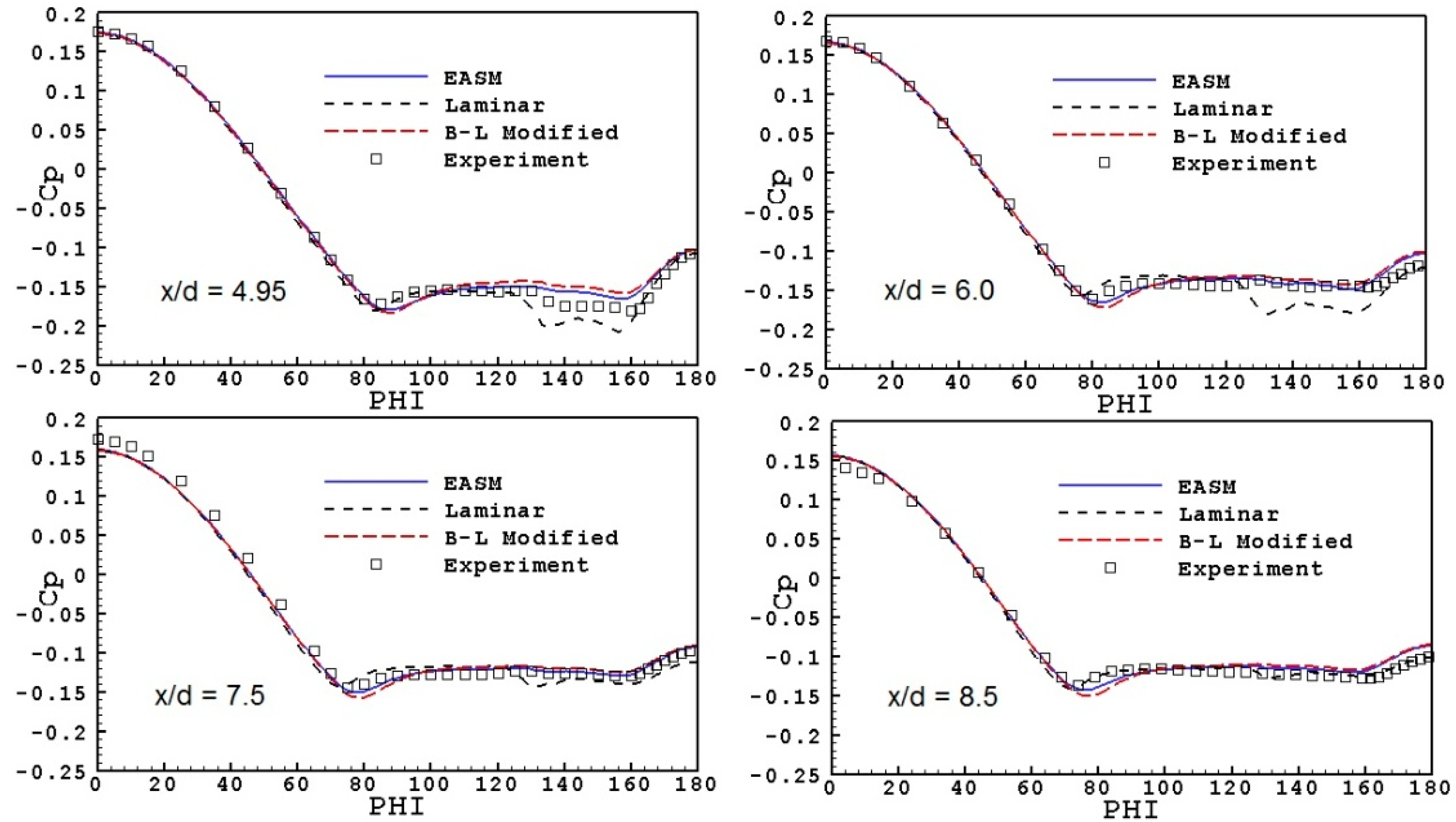
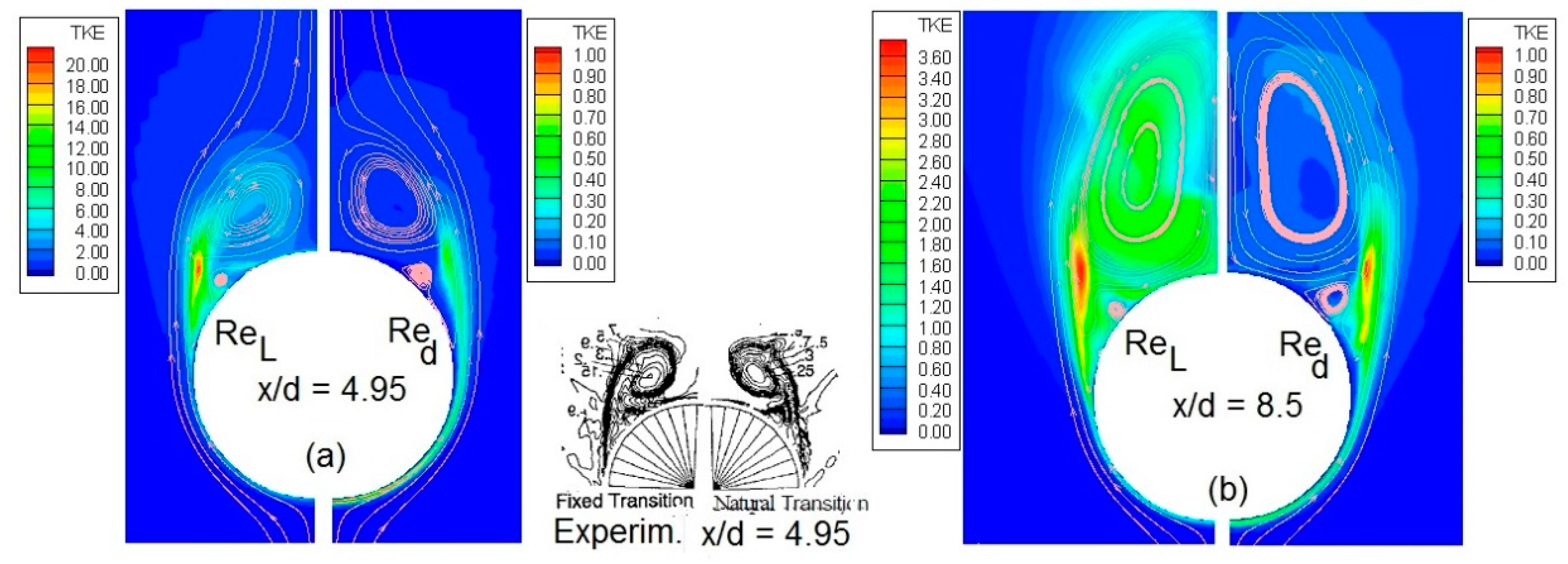
Since the high-alpha flow around wings and slender bodies is also characterized by the appearance of longitudinal separation vortices, the supersonic flow around an ogive cylinder at high-incidence has been simulated by employing the k–ω turbulence model, an Explicit Algebraic Reynolds Stress Model (EASM) and a modified Baldwin–Lomax model. All these turbulence models provided results of accepted accuracy, with the EASM model demonstrating better performance. Subsequently, the turbulent flow calculations were repeated with the arbitrary assumption that the Reynolds number in these new simulations was based on the diameter, not on the length of the body (scaling of the Reynolds number by the length of the body). Then, the predicted wall pressure distribution approached the data closer. Simultaneously, the turbulent kinetic energy in the reversed flow (EASM model) was reduced at very small levels. Of course, we do not suggest the arbitrary scaling of the Reynolds number for better accuracy. Our numerical test aimed at demonstrating that turbulent flow simulations which result in almost laminar flow conditions within the reversed flow of the separation domain, provide accurate results. A task of future efforts would be the development of turbulence models that predict flows with characteristics similar to those described in this article.