Spectral-Aware Distributional Forecasting for Risk-Aware Resource Allocation in LEO Satellite Networks

Abstract

Centralized reactive orchestration in Low Earth Orbit (LEO) networks struggles with heavy-tailed traffic surges that trigger signaling storms and topology instability. To address this challenge, we develop a LEO-specific predictive resource allocation framework that integrates spectral-aware distributional forecasting with risk-aware allocation. The forecasting module pairs cascaded dual-scale Exponential Moving Average (EMA) decomposition with a direct multi-step decoder to suppress autoregressive error accumulation. A Spectral Penalty operating in the frequency domain enhances sensitivity to orbital harmonics, while nonuniform quantization yields calibrated probabilistic bounds that preserve heavy-tailed characteristics. On the allocation side, the predictive standard deviation serves as an endogenous risk index amplified by service priority to form a capacity bound that is explicitly aware of risk. A companion demand model structurally reserves a fixed control plane bandwidth floor, insulating signaling from data plane congestion. Simulation results show that the forecasting module reduces the Continuous Ranked Probability Score (CRPS) by up to 5.9% relative to the strongest compared distributional baseline across prediction horizons of 30–105 min. Under a 300% traffic shock, the distributed allocation mechanism maintains 99.99% satisfaction for the highest priority service class and keeps control plane overflow below 0.05%. Lower-priority traffic is curtailed through compression governed by priority, and the per-node memory consumption is sufficiently low for deployment on current onboard satellite processors.

1. Introduction

As Low Earth Orbit (LEO) mega constellations move from design studies into commercial service, the ability to orchestrate onboard resources dynamically has become essential for keeping connectivity alive across topologies that reconfigure in the order of minutes [1,2]. Satellites at LEO altitudes complete an orbit in roughly ninety minutes, so handovers are frequent and the control plane faces persistent pressure to reconfigure. Orchestration schemes built around centralized ground loops struggle under these conditions: tracking windows are brief, telemetry round trips add nonnegligible delay, and the resulting reactive posture falls behind the pace of topology change [3,4]. The situation worsens when unexpected data plane surges saturate shared onboard buffers, because keepalive and routing protocol messages may then be delayed or lost altogether, opening the door to cascading reconvergence across neighboring nodes [5,6].

One way to ease this reactive bottleneck is to adopt a proactive, forecast-driven orchestration paradigm that prepositions resources ahead of demand spikes [7,8]. Realizing such a paradigm in LEO networks is far from straightforward, however. Traffic profiles on these platforms are shaped by two coupled periodicities—the orbital revolution and the diurnal activity cycle—and simultaneously exhibit heavy-tailed burst distributions; the extreme quantiles of those bursts are what ultimately drive Service Level Agreement (SLA) violations [9]. Deterministic point predictors trained under Mean Squared Error (MSE) objectives converge toward the conditional mean, thereby smoothing out the heavy-tailed peaks that the orchestrator most needs to see [10]. Uncertainty Quantification (UQ) methods have tried to fill this void by producing predictive intervals, yet each family carries its own limitations. Quantile regression is assumption-free in principle, but the scarcity of observations in the distribution tails inflates its estimation variance at the very quantile levels relevant to SLA enforcement. Conformal prediction shares this assumption-free appeal yet yields intervals that grow so wide under heavy-tailed arrivals as to lose practical utility [11]. Parametric Bayesian approaches face the reverse difficulty: they require an explicit likelihood form, and the skewed, non-Gaussian loads typical of LEO traffic violate those distributional premises [12,13]. Producing calibrated distributional forecasts that track extreme quantile behavior under nonstationary orbital dynamics thus remains an open problem in the satellite networking literature.

Even supposing that a reliable distributional forecast was available, a separate and less studied problem remains: how to translate the resulting statistical quantities into actual capacity decisions. The forecasting module outputs an expectation and a predictive uncertainty estimate at the scheduling interval timescale, yet the orchestrator must lock in deterministic bandwidth allocations whose consequences play out at the packet level within each interval. LEO onboard processors work within stringent power and computation budgets, and inter-satellite links frequently multiplex control and data traffic onto the same physical channel [14,15]. Under these conditions, a sudden data plane surge can fill the constrained link-layer buffer at the Medium Access Control (MAC) sublayer before any higher-layer scheduler has an opportunity to react, so both data packets and signaling messages are dropped indiscriminately. Converting predictive uncertainty into a capacity bound that accounts for risk while structurally shielding control plane signaling is a question that the literature has barely begun to address. These two open issues are not independent of each other. Risk-aware sizing depends on a calibrated distributional forecast, which in turn is only useful if the resulting uncertainty can be mapped to concrete capacity decisions.

Existing studies have attempted to alleviate the operational difficulties of LEO networks through network orchestration, traffic prediction, and resource allocation. Software-Defined Networking (SDN) and Virtual Network Function (VNF) orchestration can coordinate service provisioning and resource management, thereby improving the adaptability of dynamic satellite networks [2]. Nevertheless, their performance depends on timely telemetry collection and control execution, which can be difficult under short contact windows and rapidly changing inter-satellite links. Traffic prediction has therefore been introduced to support proactive resource planning before congestion occurs [16]. However, existing deterministic prediction studies often emphasize average error measures, so the tail behavior of traffic bursts associated with SLA violations may receive limited attention. Probabilistic forecasting and UQ further provide intervals, quantiles, or distributional descriptions of future traffic [11]. These outputs must still be transformed into bandwidth decisions before they can directly support onboard scheduling. Recent studies on resource allocation under uncertainty have also introduced risk-related formulations to maintain Quality of Service (QoS) in LEO satellite networks [17]. However, how distributional traffic information should be used when setting capacity margins for different service priorities remains an issue requiring further investigation. Therefore, this study focuses on the connection between distributional traffic forecasting and risk-aware bandwidth sizing for LEO satellite networks, where both average load and extreme demand fluctuations affect SLA satisfaction under constrained onboard resources.

Motivated by the above challenges, this paper develops an LEO-specific predictive resource allocation framework, termed Spectral-Aware Distributional Resource Allocation (SADRA), for nonstationary and bursty satellite traffic. Figure 1 depicts a representative constellation scenario in which heterogeneous service classes share time-varying inter-satellite links under these constraints. The major contributions are summarized as follows:

• We develop a spectral-aware distributional forecasting approach for nonstationary and bursty LEO traffic. This approach adapts the dual-scale Exponential Moving Average (EMA) decomposition to orbital and diurnal periodicities, with spectral regularization and equiprobable inverse Cumulative Distribution Function (CDF) quantization incorporated to characterize the distributional features of satellite traffic.
• Different from deterministic allocation schemes that rely mainly on point traffic prediction, predictive mean and standard deviation are jointly used to calculate bandwidth margins according to service priority, which are combined with a control-plane bandwidth floor to protect signaling traffic during congestion.
• A series of experiments are conducted to assess both forecasting performance and allocation resilience, covering forecasting accuracy and calibration, priority-based allocation, and scalability across different constellation configurations.

The remainder of this paper is organized as follows: Section 2 reviews related studies on LEO network orchestration, traffic prediction, probabilistic forecasting, and resource allocation, and clarifies the position of this study within the literature. Section 3 presents the spectral-aware distributional forecasting model for capturing periodic variations and bursty traffic behavior. Section 4 describes the conversion of the predictive mean and standard deviation into priority-aware bandwidth allocations for congested LEO links. Section 5 reports the numerical experiments and discusses the forecasting and allocation results under representative constellation settings. Finally, Section 6 summarizes the main conclusions and outlines future work.

2. Related Work

Work on LEO resource management generally tackles the allocation problem from two complementary angles: formulating capacity orchestration across service classes, and predicting the underlying traffic demand through spatiotemporal models [18].

2.1. Dynamic Resource Orchestration

Satellite network slicing enabled by SDN and Network Function Virtualization (NFV) is typically cast as a nondeterministic polynomial-time hard (NP-hard) joint optimization problem [19]. Exact solvers that rely on convex relaxation or Mixed-Integer Linear Programming (MILP) can, in principle, guarantee global optimality; yet, their worst-case complexity grows exponentially with the number of binary decision variables, rendering them impractical when onboard scheduling deadlines are tight. Metaheuristics such as Genetic Algorithms and Ant Colony Optimization run within a controllable per-iteration budget, but the time they need to converge to a feasible solution is hard to bound in advance, and the resulting allocations carry an optimality gap that provides no formal assurance of meeting physical hard constraints in every scheduling instance. Both families of limitations narrow the applicability of these methods to the tight onboard scheduling deadlines that LEO topologies impose.

Given these scalability concerns, a number of recent studies have moved toward allocation methods in closed form that are conditioned on predictive inputs [14]. Distributed control has also attracted growing interest, with several proposals targeting the coordination of slice resources across cells [20] and the joint allocation of bandwidth and compute [21], as well as reinforcement-learning-driven distributed routing in mega-constellation networks [22]. Beyond these analytical approaches, scheduling policies grounded in learning have been explored as a way to adapt to time-varying service demands without solving an explicit optimization at each step [23,24]. Separately, Digital Twin (DT) assisted frameworks build a virtual replica of the constellation to emulate candidate allocation decisions before committing them to the live network, thereby absorbing much of the prediction uncertainty offline [25]. Both learning-based strategies and twin-assisted strategies offer strong adaptive capabilities under moderate loads, yet neither explicitly addresses how control plane signaling should be protected when aggregate demand exceeds the physical link capacity. On LEO platforms where per-hop QoS enforcement remains limited, a proactive capacity reservation introduced at the slice admission stage is necessary to structurally preserve signaling bandwidth during traffic spikes.

A related body of work formulates the slicing problem under explicit demand uncertainty. Stochastic Network Calculus derives analytical delay and backlog bounds that support probabilistic service guarantees [26], while programming with chance constraints expresses SLA targets as probabilistic capacity constraints and reformulates them via Bernstein or Conditional Value-at-Risk (CVaR) approximations to obtain convex programs [17]. Robust optimization hedges against worst-case demand within a specified uncertainty set and has been applied to LEO slice admission under time-varying topology [27]. For moderate problem dimensions, these formulations can run on current processors hardened against radiation; yet their per-interval solve time scales with the number of coupled slices and constraints, making online execution difficult when the onboard scheduling window is on the order of seconds and the energy budget is tightly constrained. The closed-form allocation derived in Section 4 sidesteps this solver dependency by translating predictive standard deviation directly into a capacity bound in $\mathcal{O}(KlogK)$.

2.2. Traffic Forecasting and Uncertainty Quantification

Classical time series methods such as Autoregressive Integrated Moving Average (ARIMA) [28] and Markov Modulated Poisson Processes [29] rest on assumptions of stationarity and short-range dependence; neither assumption holds under orbital periodicity and the load shifts that handovers induce.

By relaxing the linearity constraint, deep sequence models like Long Short-Term Memory (LSTM) networks and Gated Recurrent Unit (GRU) models [30] have achieved improved accuracy on bursty traffic traces. Subsequent research introduced spatiotemporal graph architectures that jointly model temporal dynamics across constellation nodes, capturing load variations at each node under discrete topology snapshots [31,32]. More recently, advanced Transformer designs—PatchTST [33] and multiscale mixing strategies [34]—treat subseries patches as tokens and fuse information across multiple temporal resolutions, extending point prediction capabilities on long horizon benchmarks. To counteract the spectral bias that MSE-optimized models exhibit, some researchers have turned to representations in the frequency domain; penalizing discrepancies in the Fourier spectrum has been shown to noticeably sharpen sensitivity to periodic elements such as the orbital harmonic and to transient bursts [35]. Most spatiotemporal models nonetheless confine their outputs to deterministic point estimates, leaving the distributional nature of future demand unaddressed.

In parallel, a growing line of work has concentrated on integrating uncertainty quantification (UQ) into time series forecasting. Representative techniques span quantile regression [36], Gaussian processes, Bayesian neural networks, and conformal prediction [37]. By minimizing scoring rules such as the Continuous Ranked Probability Score (CRPS) or the energy score, models can be steered to output full predictive distributions instead of simple point summaries [38]. Among these techniques, Bayesian neural networks and Gaussian processes typically embed parametric likelihood assumptions that may not fit heavy-tailed residuals well. Quantile regression and conformal prediction, in contrast, do not require distributional assumptions; yet at the extreme quantile levels that matter most for SLA enforcement, quantile regression suffers from data sparsity and quantile crossing instabilities, while conformal prediction produces intervals that grow uninformatively wide under heavy-tailed arrivals [12,13].

Taken together, the studies most relevant to predictive LEO resource allocation can be organized around two closely related themes: resource orchestration under limited satellite capacity and traffic prediction under nonstationary demand. Since predictive allocation draws on both streams,

Table 1. Comparison of representative approaches for LEO traffic forecasting and resource allocation.

Approach	Representative Methods	Applicability	Limitations
Resource allocation approaches
Mathematical optimization	MILP, convex optimization, decomposition methods	Well suited to offline planning and small-scale cases where explicit constraints and interpretable decisions are required	Repeated fine-grained solving becomes costly as service slices, decision variables, and topology constraints grow
Heuristic and metaheuristic allocation	Greedy heuristics, genetic algorithms, ant colony optimization	Useful for exploratory optimization and parameter tuning in large or nonconvex allocation spaces	Convergence behavior and final optimality gaps are often difficult to guarantee a priori
Learning-based orchestration	Reinforcement learning, deep reinforcement learning, multi-agent reinforcement learning	Promising for dynamic orchestration because policies can be learned from traffic and topology states	Policy quality depends on training coverage, reward design, and validation under unseen congestion or topology changes
Uncertainty-aware resource allocation	Stochastic network calculus, chance constraints, robust optimization	Relevant to SLA-aware allocation because demand uncertainty can be expressed through probabilistic or worst-case service requirements	Practical value depends on the uncertainty model or uncertainty set, and frequent online re-optimization may add overhead
Traffic forecasting approaches
Point traffic forecasting	ARIMA, LSTM, GRU, spatiotemporal graph models, Transformer models	Useful for demand tracking and capacity planning through temporal or spatiotemporal demand estimates	Point estimates alone do not describe uncertainty or tail risk during traffic bursts
Probabilistic traffic forecasting	Quantile regression, Gaussian process regression, Bayesian neural networks, conformal prediction	More informative for risk-aware planning because intervals, quantiles, or predictive distributions can be obtained	LEO use still requires validation under orbital periodicity, handover-induced load shifts, and heavy-tailed bursts

summarizes representative method families in two groups: resource allocation approaches and traffic forecasting approaches. The categories reflect the dominant modeling perspective of each group; in practice, several studies may combine more than one perspective.

Table 1 shows that existing approaches have made substantial progress in both resource allocation and traffic forecasting, but their integration remains limited in LEO resource allocation under rapidly varying demand. In the allocation group, optimization and heuristic methods mainly address feasibility and tractability, learning-based methods offer greater adaptability when sufficient training coverage is available, and uncertainty-aware formulations introduce probabilistic or worst-case service considerations. Their practical performance, however, may depend on repeated optimization, training generalization, distributional assumptions, or prescribed uncertainty sets. In the forecasting group, point forecasting methods provide useful demand estimates, while probabilistic forecasting methods further describe uncertainty; yet their connection to computationally practical resource allocation in dynamic LEO networks remains limited. These observations indicate a remaining need for LEO resource-allocation studies to more closely connect traffic forecasts with uncertainty information, so that the application difficulties caused by demand bursts, prediction errors, and recurrent topology changes can be mitigated without sacrificing computational practicality.

Achieving calibrated distributional outputs together with heavy-tail robustness over dynamic satellite graphs consequently remains an open problem in LEO resource allocation.

3. Spectral-Aware Distributional Forecasting

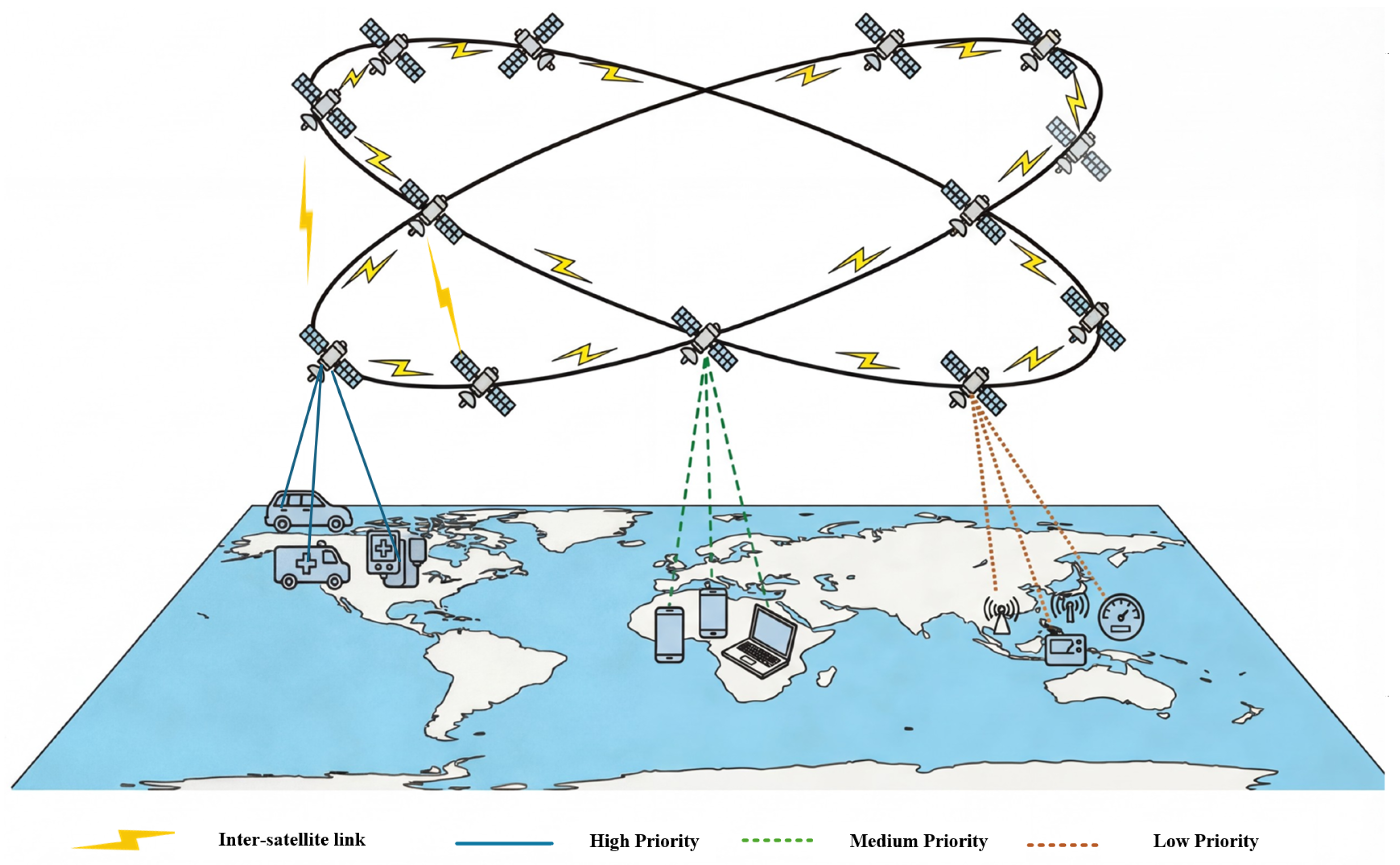
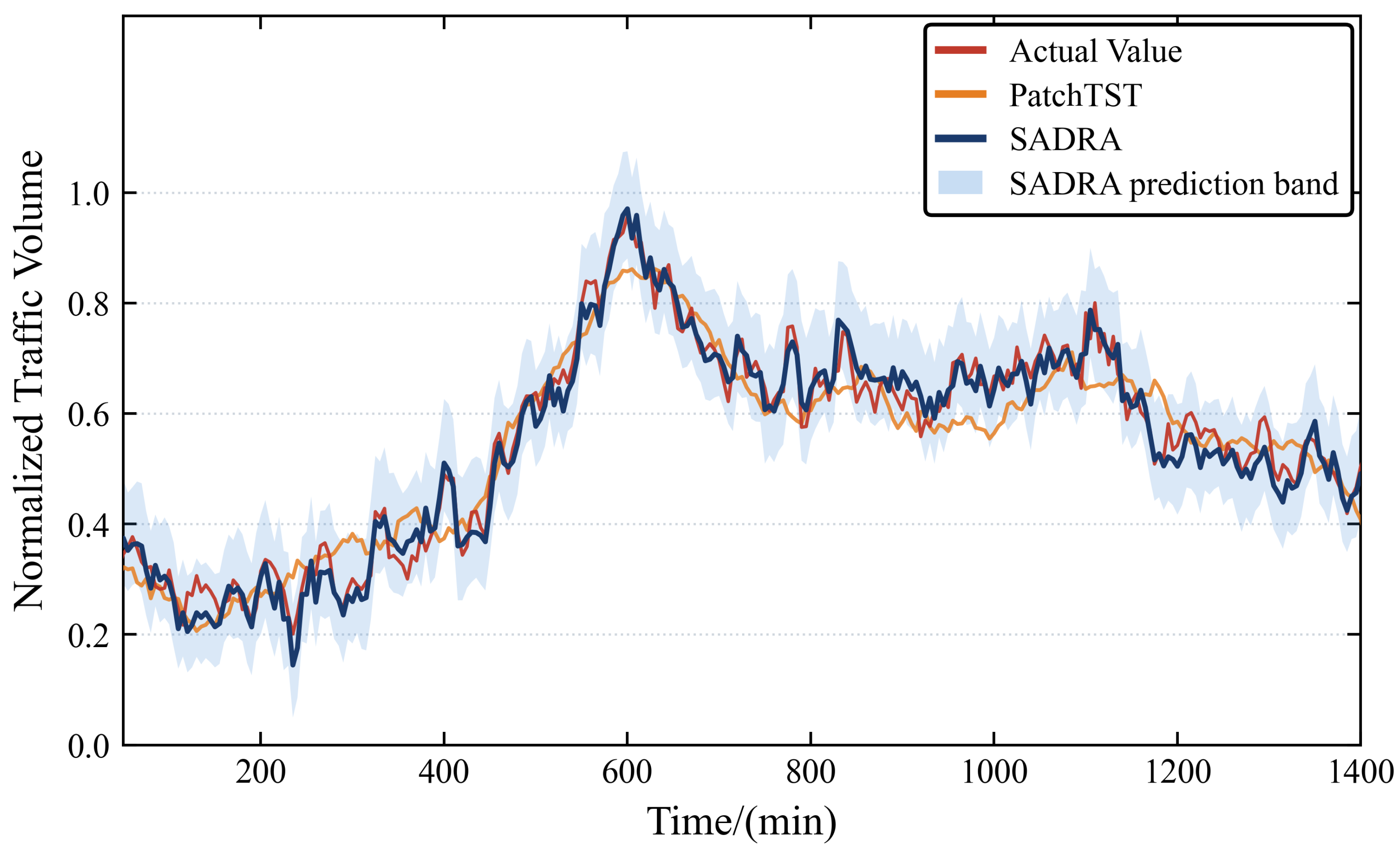
Consider an LEO constellation of N satellite nodes connected through a time-varying Inter-Satellite Link (ISL) graph. At each time step t, the aggregated nodal traffic ${\mathbf{X}}^{\left(t\right)}\in {\mathbb{R}}^{N\times d_f}$ displays coupled periodicity at two scales: the orbital period $T_{orb}$ and the diurnal cycle [8]. Multiscale temporal mixing [34] can handle such nonstationarity; yet point predictors trained under MSE converge to the conditional mean and thereby attenuate heavy-tailed peaks.

To move beyond this limitation, SADRA is organized into three stages: an interleaved backbone with temporal decoupling using independent channels, regularization in the frequency domain through a spectral penalty, and equiprobable discrete support set mapping combined with distributional fusion weighted by confidence. Figure 2 shows the complete architecture.

3.1. Dual Branch Backbone and Temporal Decomposition

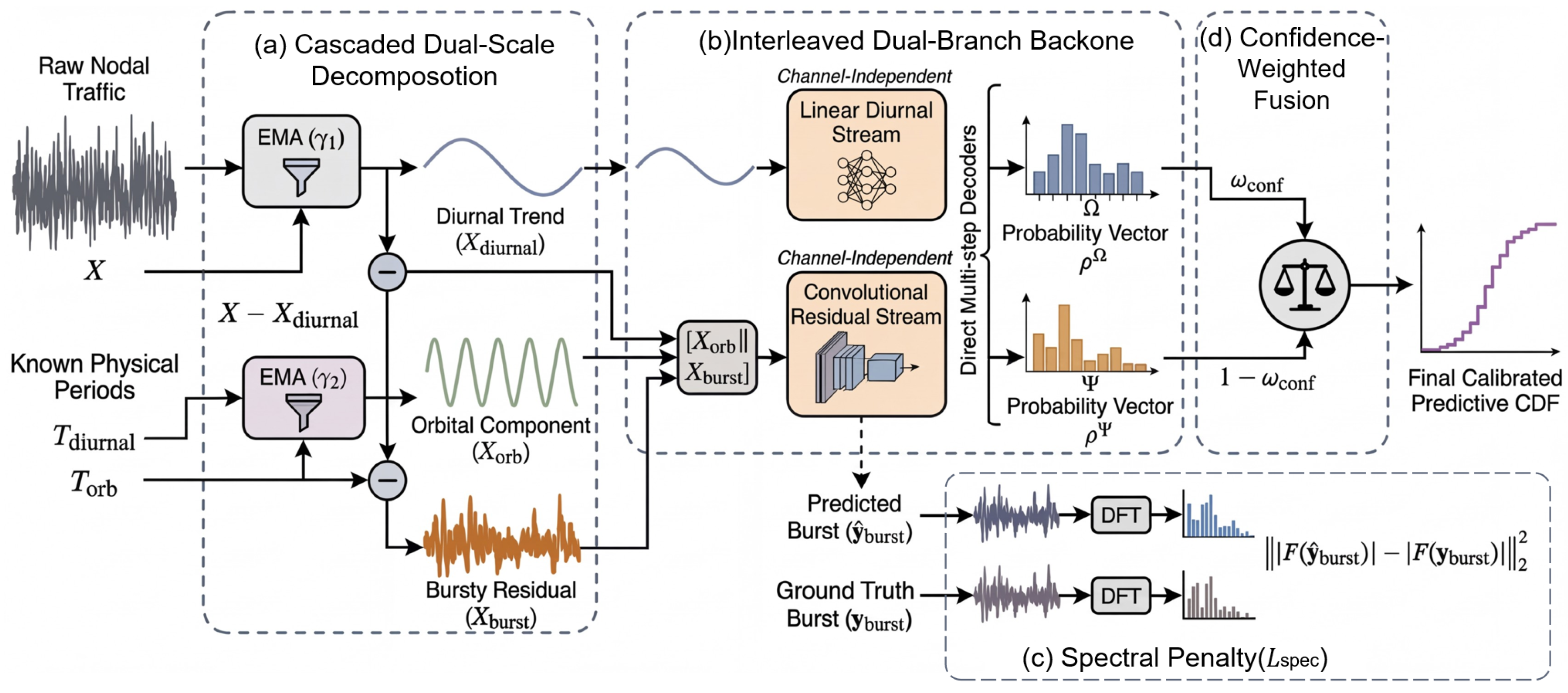
We decompose the observed traffic into three components through a cascaded dual-scale EMA scheme. Let $\mathbf{X}\in {\mathbb{R}}^{T_{obs}\times d_f}$ denote the historical traffic series at a given node, where $d_f$ is the feature dimension and $T_{obs}$ is the lookback window.

Building on prior single-scale decomposition designs, our approach further exploits the a priori knowledge that LEO traffic is simultaneously governed by two distinct physical periods: the diurnal cycle $T_{diurnal}=1440$ min, fixed by Earth’s rotation, and the orbital period $T_{orb}$ specific to each constellation, obtained from Systems Tool Kit (STK) orbital propagation. The cascaded decomposition takes the following form:

$$\left\{\begin{array}{c}{\mathbf{X}}_{diurnal}=\mathrm{EMA}(\mathbf{X},{\gamma }_1)\hfill \\ {\mathbf{X}}_{orb}=\mathrm{EMA}(\mathbf{X}-{\mathbf{X}}_{diurnal},{\gamma }_2)\hfill \\ {\mathbf{X}}_{burst}=\mathbf{X}-{\mathbf{X}}_{diurnal}-{\mathbf{X}}_{orb}\hfill \end{array}\right.$$

(1)

The smoothing factors are tied directly to the physical periods instead of being treated as free hyperparameters. Following the standard EMA window–smoothing relation:

$${\gamma }_1={\displaystyle \frac{2}{T_{diurnal}/\Delta t+1}}$$

(2)

$${\gamma }_2={\displaystyle \frac{2}{T_{orb}/\Delta t+1}}$$

(3)

where $\Delta t$ is the sampling interval. For $\Delta t=5$ min and a medium-scale constellation of 298 satellites at 1015 km altitude with $T_{orb}=105$ min, one obtains ${\gamma }_1=0.007$ and ${\gamma }_2=0.091$. Here, the diurnal trend ${\mathbf{X}}_{diurnal}$ captures the slowly evolving ground demand pattern; the orbital component ${\mathbf{X}}_{orb}$ isolates the periodic oscillation induced by coverage changes; and the residual ${\mathbf{X}}_{burst}$ represents the heavy-tailed bursty traffic that is most responsible for SLA violations. With ${\gamma }_1=0.007$, the diurnal branch effectively operates as a low pass filter that spans multiple revolutions and tracks baseline drift at the day scale, while the rapid dynamics driven by coverage are absorbed by ${\gamma }_2$ and the burst residual.

Given this decomposition, an Interleaved Dual Branch Backbone processes both scales in parallel. The orbital and burst residuals ${\mathbf{X}}_{orb}$, ${\mathbf{X}}_{burst}$ are concatenated, segmented into patches of fixed length, and encoded through a lightweight convolutional stream, while the diurnal trend ${\mathbf{X}}_{diurnal}$ passes through a linear projection. Although the two branches share an identical architecture, they maintain independent parameters, and each branch outputs a discrete probability distribution over a distinct support set—$\Omega$ or $\Psi$. To keep computation per node manageable when many service classes share the same satellite, the backbone adopts a Strategy with Independent Channels: each traffic feature is treated as a univariate input, thereby avoiding the quadratic cost that cross-channel attention would incur [8].

In this study, we follow the established direct multi-step prediction paradigm, abbreviated as Non-Iterative Direct Mapping (NDM), to circumvent autoregressive error accumulation over long horizons. Let ${\mathbf{H}}_{diurnal}\left(t\right)$ and ${\mathbf{H}}_{res}\left(t\right)=[{\mathbf{X}}_{orb}\parallel {\mathbf{X}}_{burst}]$ collect the respective lookback windows for the diurnal and residual streams. Each future step h is predicted by a dedicated decoder head that outputs a probability vector over the support set specific to its branch, $\Omega$ or $\Psi$:

$${\rho }_{t+h}^{\Omega }=\mathrm{Softmax}\left({\mathcal{H}}_{map}^{\left(h\right)}\left({\mathbf{H}}_{diurnal}\left(t\right),{\mathbf{H}}_{res}\left(t\right)\right)\right),\forall h\in \{1,2,\dots ,T_H\}$$

(4)

where ${\mathcal{H}}_{map}^{\left(h\right)}(·)$ is the decoder head for step h within the structure with independent channels and ${\rho }_{t+h}^{\Omega }\in {\mathbb{R}}^M$ assigns probability mass to each bin of $\Omega$; the staggered branch ${\rho }_{t+h}^{\Psi }\in {\mathbb{R}}^{M-1}$, corresponding to the $M-1$ intervals of $\Psi$, is obtained with an identical architecture but independent parameters. By predicting each horizon step directly, the formulation avoids error accumulation.

3.2. Spectral Penalty

Neural networks trained with objectives defined solely in the time domain develop an inherent spectral bias toward low-frequency components during gradient descent. Because the burst residual ${\mathbf{X}}_{burst}$ concentrates the transient energy that drives SLA violations, this bias is most harmful in the high-frequency band where severe traffic spikes reside.

To counter this effect, we incorporate a regularizer in the frequency domain termed Spectral Penalty, drawing on recent loss designs in the frequency domain [35]. Let $\mathfrak{F}(·)$ denote the one-dimensional Discrete Fourier Transform (DFT). The penalty measures how much the spectral amplitudes of the predicted and true dynamic components diverge, up to the Nyquist frequency:

$$L_{spec}={\displaystyle \frac{1}{\lfloor T_H/2\rfloor }}{\displaystyle \sum _{\omega =1}^{\lfloor T_H/2\rfloor }}{\left(\left|\mathfrak{F}{\left({\mathbf{X}}_{burst}^{\left(pred\right)}\right)}_{\omega }\right|-\left|\mathfrak{F}{\left({\mathbf{X}}_{burst}^{\left(true\right)}\right)}_{\omega }\right|\right)}^2$$

(5)

where $|·|$ extracts the spectral magnitude. In order to structurally preserve the high-frequency energy associated with severe transient bursts during training, the deterministic sequence ${\mathbf{X}}_{burst}^{\left(pred\right)}$ fed to the DFT is extracted through a differentiable Soft Argmax operation over the discrete support set centroids. Gradients from $L_{spec}$ thus flow through the probability-weighted centroid of the predicted distribution. The DFT coefficient at frequency $\omega$ for a sequence $\mathbf{x}\in {\mathbb{R}}^{T_H}$ is

$$\mathfrak{F}{\left(\mathbf{x}\right)}_{\omega }={\displaystyle \sum _{s=0}^{T_H-1}}{x}_s{e}^{-j{\displaystyle \frac{2\pi }{T_H}}\omega s},\omega \in \left\{0,1,\dots ,\lfloor T_H/2\rfloor \right\}$$

(6)

Note that the summation in $L_{spec}$ starts from $\omega =1$, which excludes the zero-frequency component. Normalization by $\lfloor T_H/2\rfloor$ keeps the penalty invariant to the prediction horizon length. Because ${\mathbf{X}}_{burst}$ retains near-zero mean after the cascaded EMA subtraction and the zero-frequency bin is already excluded from $L_{spec}$, the dominant source of spectral leakage is suppressed and no additional windowing is applied. $L_{spec}$ is defined on amplitude-spectrum discrepancies of the burst component and enters the total training loss in Equation (8) through a weighting coefficient ${\lambda }_{spec}$. The spectral term is not intended to serve as the sole timing constraint, because the stepwise negative log-likelihood is computed in the original time domain and penalizes temporally misaligned burst predictions. Thus, the amplitude-spectrum penalty complements the time-domain distributional loss by preserving burst-related high-frequency energy, while temporal localization remains anchored by the time-domain objective.

3.3. Quantization and Distributional Fusion

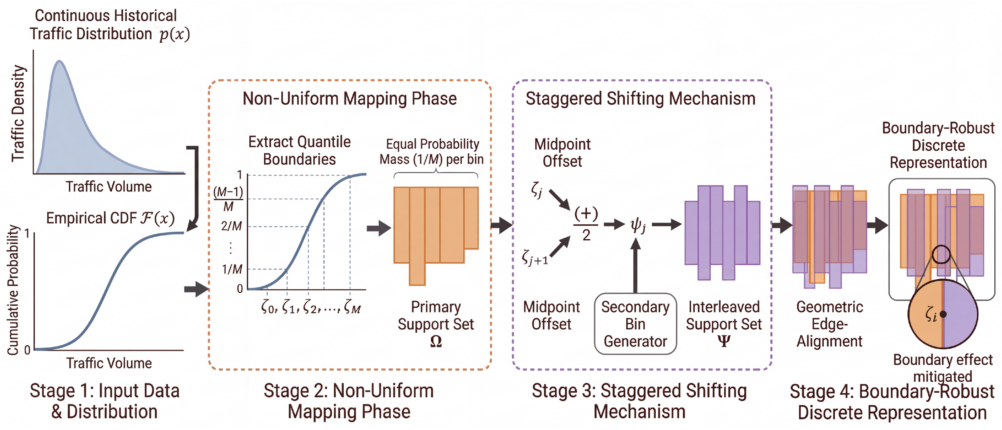
To approximate the continuous conditional distribution $p_{\theta }\left(\mathbf{y}\right|\mathbf{H})$ with a categorical output, the traffic domain must be mapped to a finite set of bins. Because uniform binning offers poor resolution in the tails, we construct a Nonuniform Support Set from the inverse CDF of the training traffic distribution.

Let M denote the number of intervals, delimited by boundary points $\{{\zeta }_0,{\zeta }_1,\dots ,{\zeta }_M\}$. These boundaries are chosen so that ${\int }_{{\zeta }_{i-1}}^{{\zeta }_i}p\left(x\right)dx=1/M$, meaning every bin carries equal probability mass, an arrangement known as equiprobable quantization. The primary support set is then $\Omega =\{[{\zeta }_0,{\zeta }_1),\dots ,[{\zeta }_{M-1},{\zeta }_M]\}$.

Both the inverse CDF and the resulting bin boundaries are computed exclusively from the training split, which prevents data leakage. Because traffic statistics vary with orbital latitude and service class, the bins are not shared globally; instead, each satellite calibrates its own support sets ${\Omega }^{\left(k\right)}$ and ${\Psi }^{\left(k\right)}$ independently for each node and class, accommodating spatial heterogeneity without any centralized recalibration step.

Whenever the true traffic value falls near a bin boundary ${\zeta }_i$, probability mass can leak to adjacent bins, distorting the reconstructed expectation.

To mitigate this boundary effect explicitly, we introduce a second staggered support set $\Psi$ whose boundaries are offset to the midpoints of the primary bins:

$${\psi }_j={\displaystyle \frac{{\zeta }_j+{\zeta }_{j+1}}{2}},\forall j\in \{0,1,\dots ,M-1\}$$

(7)

These M midpoints delimit $M-1$ staggered intervals, giving $\Psi =\{[{\psi }_0,{\psi }_1),\dots ,[{\psi }_{M-2},{\psi }_{M-1}]\}$. By staggering the bins in this way, the worst-case discretization error at bin edges is reduced, and the combined system can approximate continuous distributions with a moderate number of bins, as illustrated in Figure 3.

The complete training objective combines the Negative Log-Likelihood (NLL) with the spectral regularizer:

$$\mathcal{L}={\mathcal{L}}_{NLL}+{\lambda }_{spec}{L}_{spec}$$

(8)

where ${\lambda }_{spec}=0.1$ is chosen by grid search on the validation set.

Outputs from the two interleaved branches are fused to construct an empirical CDF, $\widehat{F}\left(y\right)$. The two branch distributions are not collapsed to a single expectation; instead, each node computes a cumulative sum weighted by confidence over both branch probability masses. Let ${\rho }^{\Omega }$ and ${\rho }^{\Psi }$ be the softmax-normalized probability vectors for the primary and staggered support sets, respectively. The fusion weight ${\omega }_{conf}\in (0,1)$ is defined as the normalized peak probability of the primary branch: ${\omega }_{conf}={max}_m{\rho }_m^{\Omega }/({max}_m{\rho }_m^{\Omega }+{max}_m{\rho }_m^{\Psi })$, which gives a larger weight to whichever branch is sharper, i.e., more confident. The fused empirical CDF evaluated at traffic volume y is then

$$\widehat{F}\left(y\right)={\omega }_{conf}{\displaystyle \sum _{m=1}^{M_{\Omega }\left(y\right)}}{\rho }_m^{\Omega }+(1-{\omega }_{conf}){\displaystyle \sum _{m=1}^{M_{\Psi }\left(y\right)}}{\rho }_m^{\Psi }$$

(9)

where $M_{\Omega }\left(y\right)$ and $M_{\Psi }\left(y\right)$ identify the ordinal indices of the support set bins containing y.

To extract closed-form moments, the centroids of all $\Omega$ and $\Psi$ bins are collected into a sorted union. Each centroid inherits a probability mass weighted by branch confidence:

$${\widehat{\rho }}_m=\left\{\begin{array}{cc}{\omega }_{conf}·{\rho }_m^{\Omega },\hfill & \mathrm{if}{c}_m\in \Omega \hfill \\ (1-{\omega }_{conf})·{\rho }_m^{\Psi },\hfill & \mathrm{if}{c}_m\in \Psi \hfill \end{array}\right.$$

(10)

The predictive expectation and variance then follow as

$${\widehat{y}}_{t+h}=\sum _m{c}_m{\widehat{\rho }}_m{\sigma }_{t+h}^2=\sum _m{(c_m-{\widehat{y}}_{t+h})}^2{\widehat{\rho }}_m$$

(11)

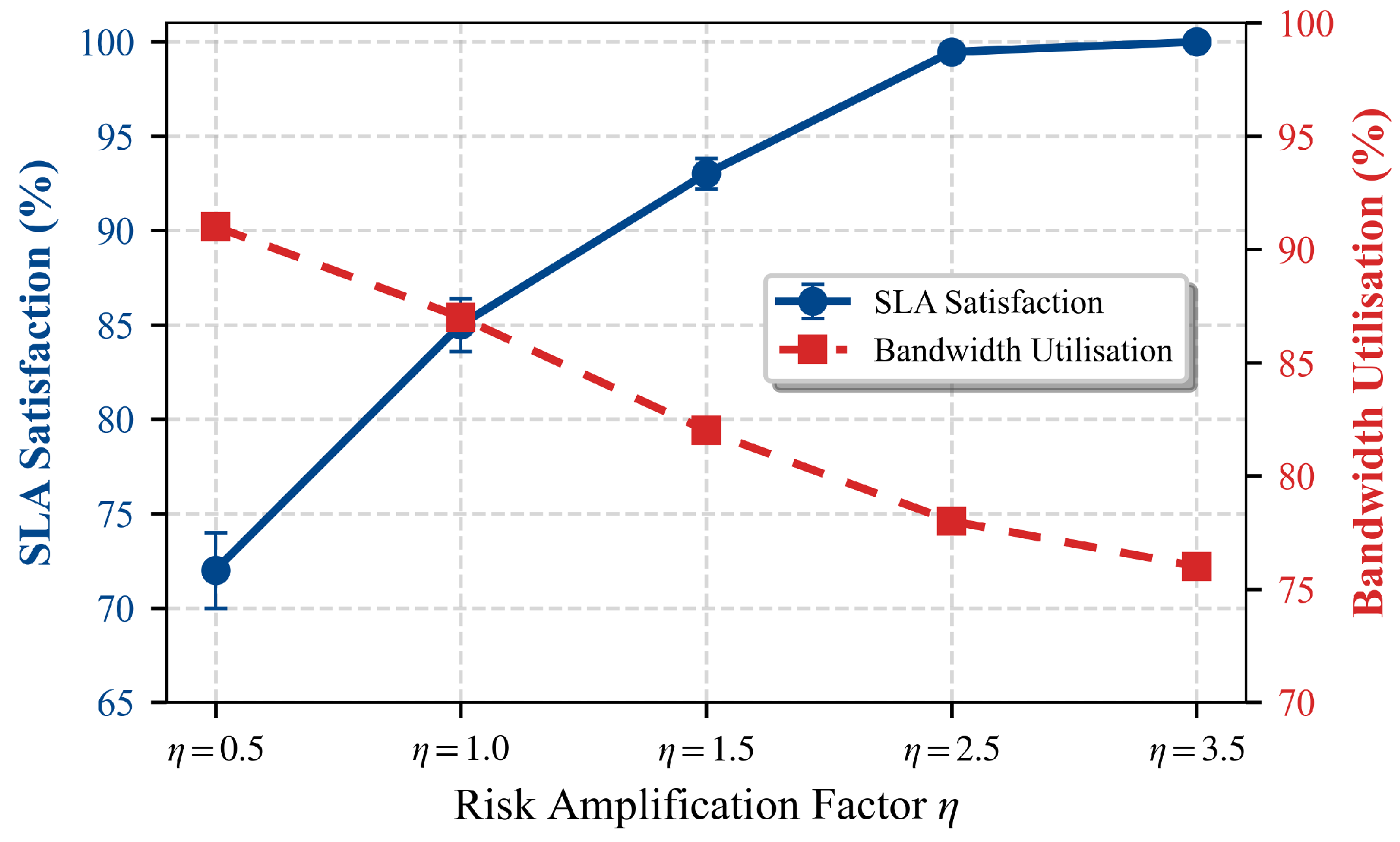
where $c_m$ is the centroid of bin m and ${\widehat{\rho }}_m$ is the fused probability mass. In this formulation, $\widehat{y}$ serves as the point forecast for capacity sizing, while ${\sigma }^2$ quantifies the intrinsic predictive uncertainty. The risk-aware allocation mechanism described in Section 4 uses its square root $\sigma$ as an endogenous risk index for each service class. Because the allocator recomputes these moments every $\Delta t$, meaning that the scheduling interval matches the forecasting sampling interval, each resource allocation decision is conditioned on the most recent distributional output.

The practical value of conditioning allocation decisions on the most recent distributional output lies in the paired estimates that it provides for each service class: near-term demand and predictive uncertainty. The demand estimate represents the nominal load expected during the next scheduling interval, while the standard deviation summarizes the short-term variability associated with bursty and heavy-tailed arrivals. This distinction matters in LEO satellite nodes because traffic surges can increase shared onboard-buffer pressure before delayed control signals clearly reveal congestion. Feeding the paired forecast to the allocator allows bandwidth margins to reflect both expected load and traffic fluctuation, easing resource-allocation pressure under constrained onboard capacity.

4. Risk-Aware Resource Allocation

From the distributional forecast in Section 3, each satellite node receives the predictive expectation ${\widehat{y}}_k$ and variance ${\sigma }_k^2$, as defined in Equation (11) for every active service class. Converting these distributional profiles into deterministic capacity decisions calls for a mechanism that (i) quantifies the intrinsic risk embedded in the prediction, (ii) maps that risk to a bandwidth margin scaled by service priority, and (iii) compresses allocations when aggregate demand exceeds the onboard link capacity. In conventional LEO configurations where ground stations orchestrate the network [4], delayed control plane adaptations let data surges exhaust shared onboard buffers, causing signaling starvation and topology instability [39]. The remainder of this section formulates an autonomous allocation pipeline that eliminates this dependence on ground loop intervention.

4.1. Risk-Aware Capacity Sizing

For each active service class k on a given satellite node, the predictive standard deviation ${\sigma }_k$ extracted in Equation (11) serves as an endogenous risk index, quantifying the residual uncertainty about forthcoming traffic intensity within the current scheduling interval $\Delta t$. Under heavy-tailed arrivals, the conditional variance exceeds what a Gaussian model would predict, so an allocation based solely on the expectation ${\widehat{y}}_k$ leaves an inadequate margin for extreme surges.

We accordingly construct a risk-aware capacity upper bound by augmenting the point forecast with a margin proportional to the predictive uncertainty:

$$h_{up}^{\left(k\right)}={\widehat{y}}_k+{\eta }_k·{\sigma }_k$$

(12)

where ${\eta }_k>0$ is a risk amplification factor calibrated to the SLA priority of service class k. Setting ${\eta }_k$ higher widens the safety margin, thereby reducing the probability that actual traffic exceeds the provisioned capacity, at the cost of lower bandwidth utilization.

Table 2. Representative risk amplification factors ${\eta }_k$ for different service priority levels.

Priority	${\mathit{\eta }}_{\mathit{k}}$	Design Objective
High	2.5–3.0	Conservative margin for critical services
Medium	1.5–2.0	Balanced reliability and efficiency
Low	0.5–1.0	Maximizes throughput utilization

lists representative ${\eta }_k$ assignments.

Equation (12) makes the role of predictive standard deviation explicit: for two service classes that share the same priority level, i.e., ${\eta }_k={\eta }_j$, the class with higher predictive uncertainty automatically receives a proportionally wider bandwidth margin. This uncertainty-driven sizing is a primary mechanism by which distributional forecasting improves resource efficiency over point prediction.

The distributional forecast operates at the scheduling interval timescale $\Delta t$ to dimension the service rate $h_{up}^{\left(k\right)}$ of each class. Within each interval, this rate governs packet-level dynamics as a fixed parameter: a properly calibrated $h_{up}^{\left(k\right)}$ ensures that the allocated service rate exceeds the interval averaged arrival rate with high probability, reducing the risk of persistent queue buildup. Subinterval bursts are absorbed by the onboard output buffer. At the 200 Mbps egress rate the 16 MB buffer drains in approximately 0.64 s; the risk-aware rate $h_{up}^{\left(k\right)}={\widehat{y}}_k+{\eta }_k{\sigma }_k$, however, already provisions ${\eta }_k$ standard deviations above the predicted mean, so the buffer needs to absorb only residual transient spikes whose instantaneous rate momentarily exceeds $h_{up}^{\left(k\right)}$. Forecast uncertainty at macro scales is addressed by the standard-deviation-derived margin itself.

4.2. Companion Demand Modeling

For each class, the total resource budget couples the dynamic data plane demand—already scaled by the risk margin—with a static control plane reservation through a linear companion relation:

$$B_{tot}^{\left(k\right)}={\alpha }_k·h_{up}^{\left(k\right)}+{\beta }_k$$

(13)

Here, ${\alpha }_k\in (0,1]$ is the payload overhead coefficient, which captures the effective link bandwidth consumed per unit of traffic demand after VNF processing for service class k; it is profiled offline from the VNF chain specification. The term ${\beta }_k>0$ is the control plane floor: the deterministic aggregate signaling rate generated by VNF heartbeats, protocol acknowledgments, and keepalive messages at the link layer for class k. Every term is expressed in the unit of link-layer throughput, measured in Mbps.

The control plane floor ${\beta }_k$ is not a tuned hyperparameter; it is derived directly from the signaling profile of the instantiated VNFs. Its value therefore varies only with the VNF composition of a service class and requires no sensitivity tuning. For the configurations evaluated in this study, ${\beta }_k$ ranges from 0.2 to 0.5 Mbps per class, aggregating VNF heartbeat intervals of 1 s, per-flow protocol acknowledgments, and the class-proportional share of node-level keepalive traffic. During the compression driven by priority that is described below, the hard constraint $B_{tot}^{\left(k\right)}\ge {\beta }_k$ structurally insulates control plane signaling from data plane contention.

4.3. Distributed Compression by Priority

Whenever ${\sum }_{k=1}^K{B}_{tot}^{\left(k\right)}>C_{max}$, each satellite runs a local Proportional Compression procedure. Each service class carries an integer priority index $q_k\in {\mathbb{N}}^{+}$, where a larger $q_k$ denotes a lower SLA priority, i.e., $q_k=1$ corresponds to the highest priority class. Service classes are first sorted in descending order of $q_k$.

The overload resolution is framed as a lexicographic allocation problem with hard reservation constraints: bandwidth is reduced tier by tier, starting from the tier of lowest priority and moving upward, subject to

$$\begin{array}{cc}\hfill & {\displaystyle \sum _{k=1}^K}{B}_{tot}^{\left(k\right)}\le C_{max}\hfill \\ \hfill & B_{tot}^{\left(k\right)}\ge {\beta }_k,\forall k\in \{1,\dots ,K\}\hfill \end{array}$$

(14)

where the first constraint caps the aggregate link bandwidth and the second preserves the control plane floor for every class.

At each scheduling interval $\Delta t$, the onboard allocator executes a complete Risk-Aware Proactive Resource Allocation procedure: it first extracts the predictive expectation ${\widehat{y}}_k$ and risk index ${\sigma }_k$ from the distributional forecast; it then computes the risk-aware capacity bound $h_{up}^{\left(k\right)}$ using the amplification factor ${\eta }_k$ specific to each class; it forms the decoupled budget through the companion relation in Equation (13); and finally, it applies a proportional compression governed by priority that strictly preserves control plane floors whenever aggregate demand exceeds $C_{max}$.

Let $q^{*}$ denote the tier that is currently being penalized, i.e., the tier of lowest priority during compression. The data plane downscaling factor $\theta \in [0,1)$ is determined by the residual capacity:

$$B_{adj,k}=\left\{\begin{array}{cc}\left({\alpha }_k·h_{up}^{\left(k\right)}\right)·\theta +{\beta }_k,\hfill & \mathrm{if}{q}_k=q^{*}\hfill \\ {\alpha }_k·h_{up}^{\left(k\right)}+{\beta }_k,\hfill & \mathrm{if}{q}_k<q^{*}\hfill \\ {\beta }_k,\hfill & \mathrm{if}{q}_k>q^{*}\hfill \end{array}\right.$$

(15)

Should the residual prove insufficient to sustain any data plane traffic for the current tier ($\theta <0$), the tier is fully exhausted and the algorithm advances $q^{*}$ to the next occupied priority level. In the extreme case where all tiers have been reduced to their control plane floors yet ${\sum }_k{\beta }_k>C_{max}$, the algorithm terminates with a floor-only allocation; this situation means the aggregate signaling overhead alone exceeds the physical link capacity—a provisioning error to be addressed at the network design stage.

Priority sorting dominates the time complexity, giving an overall worst-case complexity of $\mathcal{O}(KlogK)$ per scheduling interval on each node, well within the computational budget of current onboard processors.

Beyond this complexity bound, the procedure executed at each satellite node is designed to mitigate resource-allocation difficulties through prediction-derived capacity margins and priority-aware compression. The uncertainty-scaled margin translates a larger predictive standard deviation into additional headroom before overload is fully observed, so burst-prone services receive a margin beyond nominal demand. If aggregate demand exceeds the available link capacity, the priority-based compression rule applies stronger compression to lower-priority traffic first, limiting the impact on high-priority services during contention. Together with the minimum control-plane reservation in the companion demand model, these steps adjust bandwidth within constrained onboard resources without depending exclusively on delayed ground-loop reactions.

5. Performance Evaluation

5.1. Simulation Setup and Traffic Generation

The simulation environment integrates STK for deterministic orbital propagation and line-of-sight (LoS) visibility analysis with a NetworkX graph layer that constructs time-varying adjacency matrices. Traffic traces are sampled at regular intervals. To validate scalability, three constellation configurations are considered, as detailed in

Table 3. Simulated satellite constellation configurations.

Constellation	Satellites	Orbital Planes	Altitude (km)
Small-scale	66	6	780
Medium-scale	298	27	1015
Large-scale	1584	72	550

. Unless stated otherwise, the results presented below correspond to the primary constellation of moderate scale.

Self-similar traffic traces are synthesized using a joint spatial and temporal traffic generator built on three core components:

• Spatial demand model:Demand is anchored to actual Earth station coordinates drawn from the STK Standard Object Database (SOD). At each epoch, a node’s aggregate demand scales in proportion to the visible station density under its footprint, a quantity that fluctuates at the orbital period as the coverage footprint sweeps across regions of varying density.
• Diurnal profile from measurements: The slowly varying daily activity pattern is derived from GÉANT European backbone traffic matrices [40]. These matrices are averaged, resampled through $C^2$ periodic splines, and shifted in time by local longitude to account for global time zone diversity.
• Stochastic burst layer: Heavy-tailed surges are introduced by multiplexing independent Pareto distributed ON/OFF sources onto the baseline, producing traffic with self-similarity and a high Hurst exponent.

SLA resilience under congestion is assessed through a SimPy queueing layer with event granularity that validates the bandwidth allocation decisions at the packet level. Since the allocation algorithm operates independently on each satellite, the queueing layer is instantiated for packet-level validation at the satellite level, and the SLA statistics are averaged over multiple Monte Carlo traffic scenarios. These repeated scenarios evaluate the operational robustness of the trained forecasting-to-allocation pipeline under independently generated traffic bursts and packet-level queueing realizations. The resulting dispersion values quantify how the online allocator behaves under the traffic and queueing variability most relevant to onboard resource management. Each downlink port features an output buffer partitioned by priority, sized to several times the bandwidth-delay product and well within the onboard memory capacity of current radiation-qualified processors. Every scheduling interval $\Delta t$, the forecasting module outputs $({\widehat{y}}_k,{\sigma }_k)$, from which the allocator computes $h_{up}^{\left(k\right)}$ and configures the service rate of each class. Within each interval the service rate is held constant; packets arrive at microsecond granularity and are served at the allocated rate, with the buffer absorbing subinterval bursts. This setup makes it possible to verify whether the risk margins derived from the predictive standard deviation translate into effective queue stability under realistic packet dynamics.

5.2. Traffic Forecasting Performance

The predictive performance of SADRA is benchmarked against five baselines listed in

Table 4. Forecasting comparison across prediction horizons on the medium-scale configuration. All traffic traces are normalized to $[0,1]$ by the training set minimum and maximum; MSE, MAE, and CRPS are given in the corresponding dimensionless units. CRPS is shown only for methods that produce distributional outputs; baselines producing only point estimates are marked with —. For ARIMA, the predictive distribution is constructed from Gaussian residuals following standard practice.

Method	T = 30 min			T = 60 min			T = 105 min
	MSE	MAE	CRPS	MSE	MAE	CRPS	MSE	MAE	CRPS
ARIMA	0.1862	0.3114	0.3091	0.2524	0.3631	0.3598	0.3809	0.4537	0.4512
LSTM-GAN	0.1131	0.2248	0.2063	0.1502	0.2618	0.2391	0.2164	0.3212	0.2988
TimesNet	0.0802	0.1849	—	0.1106	0.2171	—	0.1479	0.2553	—
PatchTST	0.0769	0.1781	—	0.1048	0.2078	—	0.1391	0.2432	—
PatchTST-QR	0.0786	0.1798	0.1608	0.1071	0.2091	0.1876	0.1418	0.2449	0.2189
SADRA	0.0737	0.1720	0.1536	0.0998	0.1997	0.1779	0.1316	0.2323	0.2060

: ARIMA, LSTM-GAN [30], TimesNet [34], PatchTST [33], and PatchTST-QR, a variant of PatchTST retrained with pinball loss.

For the chosen sampling interval $\Delta t=5$ min, results are shown at three forecasting horizons $T\in \{30,60,105\}$ min, corresponding to $\{6,12,21\}$ prediction steps, respectively. Each step yields one pair $({\widehat{y}}_k,{\sigma }_k)$ that the orchestrator consumes for capacity sizing, so a 60 min horizon provides 12 scheduling cycles of lookahead capacity. MSE and Mean Absolute Error (MAE) measure the accuracy of point predictions, while CRPS evaluates distributional calibration:

$$\mathrm{CRPS}={\int }_{-\infty }^{\infty }{\left[\widehat{F}\left(y\right)-\mathbb{I}(y\ge y_{true})\right]}^{2}dy$$

(16)

As shown in Table 4, ARIMA produces the highest errors across all horizons. Among models that output deterministic point estimates, PatchTST achieves the lowest MAE at $T=105$ min. TimesNet, which models temporal variations through adaptive analysis of multiple periodicities, ranks between LSTM-GAN and PatchTST; its general purpose periodic kernel partially captures orbital dynamics but not the targeted decomposition that physical-period priors provide. PatchTST-QR provides distributional outputs through quantile regression; its CRPS is lower than that of LSTM-GAN but remains above SADRA at all horizons, leaving heavy-tailed calibration only partially addressed. SADRA achieves the lowest CRPS at all three horizons and maintains a consistent improvement in MSE and MAE at the 60 min horizon. A Diebold–Mariano (DM) test comparing SADRA to the strongest baseline at $T=60$ min yields $p<0.05$, confirming a statistically significant improvement.

Table 5. Ablation study at $T=60$ min on the medium-scale configuration.

Method	MSE	MAE	CRPS
SADRA (full)	0.0998	0.1997	0.1779
w/o $L_{spec}$	0.1021	0.2023	0.1886
w/o Physics EMA	0.1034	0.2045	0.1829

presents the ablation study that isolates the contribution of each component. Figure 4 compares the predictive trajectories of SADRA and the deterministic baseline over a 24 h traffic cycle at the primary horizon.

As Figure 4 demonstrates, the predictive trajectory produced by SADRA tracks the nonstationary traffic burst over a full 24 h cycle spanning 1440 min. Where the deterministic baseline PatchTST shows noticeable amplitude smoothing during rapid traffic inflation, SADRA preserves the high-frequency volatility without introducing artificial lag. The accompanying shaded prediction band adjusts its width according to local uncertainty, enveloping the surge spikes; the resulting upper-bound margin is then consumed by the downstream resource allocation.

Table 5 presents two ablation variants at $T=60$ min. In the first variant, w/o $L_{spec}$, we set the spectral penalty weight to zero and retrain the model with NLL only. In the second, w/o Physics EMA, we replace the ${\gamma }_1$, ${\gamma }_2$ values derived from physics with a single learnable moving average kernel. Removing $L_{spec}$ increases CRPS, so the frequency-domain regularizer contributes measurably to calibration above NLL training alone. Replacing the physics-derived EMA with a single learnable kernel raises both MSE and MAE, isolating the benefit of anchoring decomposition to the known orbital and diurnal periods.

5.3. Allocation and Resilience

With the predictive moments $({\widehat{y}}_k,{\sigma }_k)$ supplied by the forecasting module, we compute the risk-aware capacity bound $h_{up}^{\left(k\right)}$, as defined in Equation (12), feed it into the companion demand model in Equation (13), and trigger Proportional Compression during overload. Performance is averaged over multiple Monte Carlo traffic scenarios under an instantaneous 300% traffic shock. A service class is deemed to satisfy its SLA if it meets both the latency and throughput targets. Three baselines are used for comparison: Deterministic Scalar Allocation, which uses only the conditional mean with $h_{up}=\widehat{y}$ and $\eta =0$; Static Maximum Reservation, which reserves peak historical bandwidth; and Risk Margin without Control Plane Floor, where ${\beta }_k=0$.

SLA Satisfaction.Under the scalar policy, SLA satisfaction drops to 72% during surges, because the conditional mean systematically underestimates heavy-tailed extremes. Static reservation avoids this shortfall but wastes 40% of capacity through idle bandwidth. Without a control plane floor, the risk-margin policy achieves high SLA satisfaction yet suffers control plane packet loss during congestion peaks, since data plane and control plane traffic contend for the same buffer. SADRA, combining uncertainty-driven risk margins with a guaranteed control plane floor ${\beta }_k$, sustains 99.99% SLA satisfaction for the highest priority class with $q_k=1$. Medium-priority traffic maintains above 95% satisfaction, while low-priority classes undergo intentional throughput curtailment during the shock transient through the proportional compression mechanism outlined in Algorithm 1. Figure 5 illustrates the resulting trade-off as $\eta$ is swept from 0.5 to 3.5.

Algorithm 1 Risk-Aware Proactive Resource Allocation

Input: Predictive moments $\{{\widehat{y}}_k,{\sigma }_k\}$, risk factors $\left\{{\eta }_k\right\}$, priorities $\left\{q_k\right\}$,

overhead coefficients $\left\{{\alpha }_k\right\}$, floors $\left\{{\beta }_k\right\}$, capacity $C_{max}$

Output: Adjusted final allocations $\left\{B_{adj,k}\right\}$

1:   for each service class $k\in \{1,\dots ,K\}$ do

2:       $h_{up}^{\left(k\right)}\leftarrow {\widehat{y}}_k+{\eta }_k·{\sigma }_k$

3:   for each service class $k\in \{1,\dots ,K\}$ do

4:       $B_{tot}^{\left(k\right)}\leftarrow {\alpha }_k·h_{up}^{\left(k\right)}+{\beta }_k$

5:       $B_{adj,k}\leftarrow B_{tot}^{\left(k\right)}$

6:   if ${\sum }_{k=1}^K{B}_{tot}^{\left(k\right)}\le C_{max}$ then

7:       return $\left\{B_{adj,k}\right\}$

8:   Sort service classes by priority $q_k$ (descending)

9:   $q^{*}\leftarrow {max}_k{q}_k$

10: while ${\sum }_k{B}_{adj,k}>C_{max}$ do

11:       $R\leftarrow C_{max}-{\sum }_{q_k\ne q^{*}}{B}_{adj,k}$

12:       $\theta \leftarrow \left(R-{\sum }_{q_k=q^{*}}{\beta }_k\right)/{\sum }_{q_k=q^{*}}{\alpha }_k{h}_{up}^{\left(k\right)}$

13:       if $\theta \ge 0$ then

14:          Update $B_{adj,k}$ for tier $q^{*}$ via proportional compression

15:          break

16:       else

17:          $B_{adj,k}\leftarrow {\beta }_k$ for all k in tier $q^{*}$

18:          $q^{*}\leftarrow max\{q_k:q_k<q^{*}\}$

19:          if no such $q_k$ exists then break

20:  return $\left\{B_{adj,k}\right\}$

Control Plane Protection. Control plane overflow stays below 0.05%, preventing the loss of keepalive packets. For comparison, the baseline without floor protection, where ${\beta }_k=0$, exhibits a peak overflow of 3.2% during the 300% shock. Prior topology analyses indicate that sustained keepalive loss at this level can induce cascading reconvergence across neighboring nodes [39]; the floor guarantee prevents this failure mode under the tested conditions. Data plane queues may still experience packet drops under extreme overload, because the compression algorithm intentionally curtails data plane allocations; the floor protection applies exclusively to control plane traffic.

As $\eta$ increases, SLA satisfaction of the highest priority class rises from 72% to 99.99%, while bandwidth utilisation falls from 91% to 76% because a wider uncertainty-driven safety margin is set aside. Even when $\eta$ is held constant across service classes, a class with higher predictive uncertainty ${\sigma }_k$ automatically receives a proportionally wider bandwidth margin $\eta {\sigma }_k$; this is the mechanism by which distributional forecasting, in contrast to point prediction, actively differentiates resource allocation according to risk. Across all tested configurations, control plane overflow remains below 0.05% once $\eta \ge 1.5$, indicating that the floor protection holds under the conditions examined. As noted earlier, the control plane floor ${\beta }_k$ is derived directly from the aggregate signaling rate of instantiated VNFs and varies only with the VNF composition of a service class, so no sensitivity tuning is required.

Scalability is assessed across three constellation sizes.

Table 6. Scalability across constellation sizes ($T=60$ min, 300% traffic shock). Values are reported as mean ± standard deviation over Monte Carlo traffic scenarios. The low priority SLA column reflects intentional data plane curtailment by the proportional compression under extreme overload.

Constellation	Satellites	MSE	SLA High (%)	SLA Med (%)	SLA Low (%)
Small-scale	66	0.0946 ± 0.0027	99.99 ± 0.002	96.2 ± 0.28	58.3 ± 2.04
Medium-scale	298	0.0998 ± 0.0035	99.99 ± 0.004	95.8 ± 0.36	55.7 ± 2.77
Large-scale	1584	0.1067 ± 0.0042	99.98 ± 0.005	95.1 ± 0.40	52.4 ± 3.41

reports the mean and standard deviation over Monte Carlo traffic scenarios. A marginal increase in MSE is observed at larger scales, stemming from the intensified topology dynamics and frequent handovers that inherently complicate the forecasting task.

Model training is carried out offline on a GPU workstation. Each service class is treated as a univariate series through a design with independent channels, giving an inference cost per node of $\mathcal{O}(K·T_H·M)$, where $T_H$ is the forecast horizon and M the number of support set bins. The subsequent priority-driven compression in Algorithm 1 adds only $\mathcal{O}(KlogK)$ due to the sorting step. This polynomial per-node complexity stands in contrast to centralized orchestration based on MILP, whose complexity scales exponentially in the number of binary allocation variables and is therefore prohibitive under tight onboard scheduling deadlines. Beyond the asymptotic complexity analysis, we measured the end-to-end runtime of the forecasting-and-allocation update in a CPU-only implementation test on an Intel Core i5-14600KF processor. One complete online update required 39.7 ms and had a memory footprint of 23.66 MB. With model training separated from the online stage, these measurements indicate that the forecasting-and-allocation update can be executed within the scheduling loop considered in this study.

The comparative results reported in Section 5 indicate consistent improvements in both prediction and allocation performance. SADRA achieves lower forecasting errors than the selected deterministic and distributional forecasting baselines, with the lowest CRPS among the compared models at the tested horizons. The ablation results further show that both the spectral regularizer and the physics-derived EMA decomposition contribute to the reported forecasting performance. In the allocation experiment, the proposed uncertainty-driven margin and control-plane floor improve service protection under the tested traffic shock, while the measured update cost remains compatible with interval-based scheduling.

6. Conclusions

Deterministic point prediction in LEO networks relies on conditional mean estimation and therefore struggles to capture heavy-tailed traffic surges. In this paper, we develop an LEO-specific predictive resource allocation framework for satellite networks. The framework characterizes bursty LEO traffic through physics-informed, spectral-aware distributional forecasting and carries the resulting predictive uncertainty into priority-dependent capacity margins, with a fixed bandwidth floor reserved to protect control-plane signaling.

By carrying predictive uncertainty into capacity sizing, the forecast becomes directly actionable for onboard resource allocation. The forecasting component reduced the Continuous Ranked Probability Score by up to 5.9% relative to the strongest compared distributional baseline, while the allocation mechanism maintained 99.99% SLA satisfaction for high-priority traffic and kept control-plane overflow below 0.05% under the simulated 300% traffic shock.

In future work, the proposed framework could be extended to inter-satellite coordination through the compact exchange of risk indicators and residual capacity information. Because the forecasting model and allocation rule are expressed through compact distributional statistics, this extension can retain an efficient decision structure while supporting coordinated allocation across satellites. Measured LEO traffic traces would then provide a deployment-oriented basis for evaluating the extended framework under operational traffic conditions.