Article

An Appointed-Time Control Method for Morphing Aircraft with Fragility-Avoidance Prescribed Performance


School of Astronautics, Harbin Institute of Technology, Harbin 150001, China
*
Author to whom correspondence should be addressed.
Aerospace 2026, 13(5), 441; https://doi.org/10.3390/aerospace13050441
Submission received: 3 April 2026 / Revised: 28 April 2026 / Accepted: 5 May 2026 / Published: 8 May 2026
(This article belongs to the Special Issue Control of Hypersonic Morphing Flight Vehicles)

Abstract

This paper introduces an adaptive prescribed performance control (PPC) methodology designed to achieve appointed-time stabilization for morphing aircraft. The proposed approach ensures accurate attitude tracking despite challenges posed by time-varying dynamic constraints, structural deformation perturbations, abrupt aerodynamic disturbances, and rapid variations in attitude commands. Specifically, a novel appointed-time control law is developed using the back-stepping framework to enable precise adjustment of the stabilization time. Then, an adaptive performance boundary adjustment function is introduced. This function not only constrains the system state error but also adapts based on the distance between the state error and the real-time boundary, as well as command variations. This mitigates the fragility issues associated with traditional PPC methods. To further address the ‘differential explosion’ problem, an adaptive appointed-time filter is constructed in which the filter error can be stabilized for an appointed time. The unknown and total perturbations are estimated via adaptive neural networks. The designed controller is shown to guarantee the appointed time stability for all closed-loop signals and ensure that the system state error stays inside the prescribed bounds based on the stability analysis. Lastly, numerical simulations are performed to verify the advantages and effectiveness of the proposed method.

1. Introduction

As aerospace technology advances and space exploration expands, traditional fixed-geometry aircraft often fail to achieve optimal performance across diverse flight conditions. This limitation arises because their fixed aerodynamic shapes inherently involve design compromises that may not satisfy the varied requirements of different mission profiles [1]. In contrast, morphing aircraft, by dynamically altering their external configurations, can achieve optimal aerodynamic shapes tailored to real-time mission requirements. This capability allows them to maintain peak efficiency and performance across diverse flight conditions, thereby significantly expanding their operational flight envelope, including airspace and speed range. Therefore, in recent years, morphing aircraft have taken up one of the foremost areas of research interest in numerous countries [2].
However, during the deformation maneuvering process of morphing aircraft, their structure and aerodynamic characteristics change significantly, which can exacerbate the time-varying and complexities inherent of models [3]. At the same time, the deforming wing will affect the flow field around it, forming a vortex, an end flow or other complex fluid properties, which can lead to large deviations in aerodynamic parameters from ground wind tunnel test data and increase model uncertainty. In addition, the deformation process generates an additional deformation perturbation moment, and its size is inseparable from the deformation rate and flight state. A higher attitude change rate will lead to a greater deformation perturbation moment, which can adversely affect flight control quality and stability [4,5]. Furthermore, since most deformation maneuvers are relatively short in duration, the response time requirements of the control system are more stringent. Although numerous foreign scholars have conducted research on the relationship between structural modifications and aerodynamic parameters in morphing aircraft [6,7,8], the extreme complexity of this relationship has resulted in control system designs for morphing aircraft being significantly more intricate than those for conventional fixed-wing aircraft [9].
To address the aforementioned challenges, various sophisticated control algorithms have been developed for application to morphing aircraft. They include PID control [10], linear parameter-varying control [11,12], and robust control [13], linear control methods as well as nonlinear control methods such as sliding mode control [14,15], model predictive control [16] and back-stepping control [17]. Among them, the back-stepping method has been extensively applied to morphing aircraft [18,19] attributed to its straightforward control architecture, rapid convergence, and suitability for the online control of dynamic systems [20].
However, it is pertinent to note that although these aforementioned methods enhance the control system’s performance, none of them impose constraints on the flight state or make sure that the convergence time is independent of the initial state. On one hand, for morphing aircraft undertaking missions with demanding maneuvering profiles and critical time constraints, controllers’ convergence times depend on initial errors, making it difficult to adjust the controller parameters according to mission-specific response time demands, and the slower rate of convergence can decrease a vehicle’s maneuvering performance or even lead to mission failure. Although some scholars have studied fixed-time control methods and applied them to morphing aircraft [21,22,23,24], the expression of convergence time is complicated because it is usually coupled with the parameterization process of the transient performance, so the actual parameterization process must carry out reciprocal iterations to achieve the desired convergence time and transient performance at the same time. Although MPC and optimal control methods [25,26] can also provide some control over convergence time, they require real-time solution of optimization problems, which places high demands on the computational capabilities of onboard computers. Furthermore, MPC relies on an accurate mathematical model of the controlled system. However, during flight, the aerodynamic parameters of a configurable aircraft may deviate significantly from the ideal model, leading to a substantial decline in control performance; therefore, MPC is not well-suited for morphing aircraft.
For this reason, the predefined-time method—which has a more simplified relationship between the desired convergence time and the time-dependent control parameters within the controller, without coupling to transient performance parameters—has been widely studied in the fields of reusable launch vehicles [27], flexible spacecraft [28] and unmanned vehicles [29]. In the field of morphing aircraft, ref. [30] developed an adaptive non-singular sliding mode controller for which the convergence time can be explicitly tuned by a single parameter and does not depend on the initial state. In ref. [31], a novel predetermined time-sliding mode control method for the attitude control of morphing aircraft during a large-scale morphing phase was proposed, which effectively addressed strong time variability and model uncertainty during morphing maneuvers. However, predefined-time controllers typically exhibit conservative convergence times, resulting in the system often achieving stabilization prior to the designated predefined time [32,33]. This makes precise convergence time regulation difficult to achieve, despite its critical importance for stable aircraft control. If the conservatism of the convergence time estimate cannot be reduced, then it may not only cause the actual convergence rate to be excessively fast and exacerbate the effect of additive deformation perturbations, but may also allow large peaks in instantaneous responses and waste control energy. Recently, the theory of appointed-time stabilization was proposed, which can not only define the stabilization time using one parameter but also reach preset stabilization accurately [34,35]. However, existing specified-time methods tend to realize precise regulation of the convergence time by introducing infinite gain at the specified convergence moment, which will make the singularity problem at the convergence moment [36,37]. This will lead to the actuator saturation of the aircraft during the deformation maneuver, which can seriously threaten system stability. For this reason, addressing the singularity problem inherent in appointed-time stabilization theory and applying it to morphing aircraft is a key contribution driving this paper.
On the other hand, the aircraft will be affected by multiple unknown perturbations caused by state deviations, aerodynamic uncertainties and additional deformation disturbances during the deformation maneuvering process. The magnitude of an additional deformation disturbance typically exhibits a positive correlation with state variables. Constraining the system state to ensure this disturbance remains minimal during deformation maneuvers can therefore significantly alleviate demands on the control system. Consequently, to maintain system stability and achieve smooth morphing maneuverability, imposing constraints on the system state is essential. Prescribed performance control (PPC) has become increasingly popular in aerospace to solve control problems for constrained systems because of its capacity to limit the transient and steady-state performances of response processes via predesigned funnel-type constraints [38,39,40,41]. Ref. [42] successfully applied the PPC method to morphing aircraft. Ref. [43] combined PPC with a neural network to develop a prescribed performance controller for morphing aircraft, addressing significant uncertainty and state constraint challenges.
Although the above studies have shown commendable efforts, for morphing aircraft with strong maneuverability and strong uncertainty, the fragility of the above methods becomes apparent when sudden perturbations or rapidly changing attitude commands lead to a significant increase in the state error during the morphing maneuvering process, i.e., the state error approaching the boundary or exceeding the boundary causes the singularity problem [44]. This is definitely destructive in terms of maintaining attitude stabilization for morphing aircraft, which is another key issue that inspired the contribution of this paper. For this problem, a large number of studies have been carried out in the refs. [45,46,47,48,49], which have developed PPC methods that can flexibly adjust the boundaries based on the saturation condition, thus avoiding the fragility problem. However, the PPC boundaries of the above literature are extremely sensitive to saturation information, but the occurrence of input saturation does not necessarily cause the vulnerability problem to occur, which would lead to a relaxation of the boundary conditions at the expense of additional tracking performance, while applying the saturation information for boundary conditioning also triggers the algebraic loop problem. Refs. [44,50] uses system state change information to regulate the performance boundaries; however, discontinuities in the boundary regulation term near the threshold will lead to singularity problems in the derivatives of the boundary function there.
On the basis of the above discussion, this work designs a new universal barrier function and combines a novel appointed-time stabilization theory with an adaptive neural network method to investigate an attitude stabilization tracking control technique for morphing aircraft subject to time-varying constraints, deformation perturbations, sudden aerodynamic uncertainties, and rapid changes in attitude commands. The main contributions of the method in this paper compared to most existing methods are as follows:
(1) A novel appointed-time control law is introduced. Unlike the specified-time control strategies, the time-varying gain of the control law proposed herein is bounded. This boundedness effectively overcomes the singularity problem encountered at the appointed convergence time. In addition, the first- and second-order derivatives of the time transform function in this paper are 0 at the initial moment, which effectively mitigates actuator saturation triggered by large control instructions due to the large initial error.
(2) To address the full-state constraint problem and the fragility of PPC, this paper proposes a performance function that can adaptively adjust the boundary according to the state errors and commands, which effectively avoids the singularity problem triggered by the state errors approaching/exceeding the boundary due to the sudden change in perturbations or fast-change commands. Moreover, compared to the existing adaptive boundary conditioning function, the proposed performance function in this paper is continuously differentiable and the adaptive adjustment process no longer requires information about the saturation conditions, which can effectively circumvent the non-singularity of the derivative of the performance function and the problem of algebraic looping.
(3) A barrier transformation method is proposed. Compared to traditional barrier transformations [51,52], this method can not only solve the asymmetric constraint requirement when performing unconstrained error transformation but also be applied to unconstrained systems without changing the control structure.
The subsequent sections are structured below. Section 2 introduces the morphing aircraft dynamic model and the control objectives. Section 3 details the controller design process and provides the stability analysis of the designed controller. Numerical simulations are performed, and the simulation results are analyzed in Section 4. Finally, Section 5 summarizes the key findings of this study.

2. Problem Formulation

This section introduces the dynamic model of the morphing aircraft, while the form of the adaptive boundary conditioning function proposed herein, and outlines the control objectives.

2.1. Dynamic Model

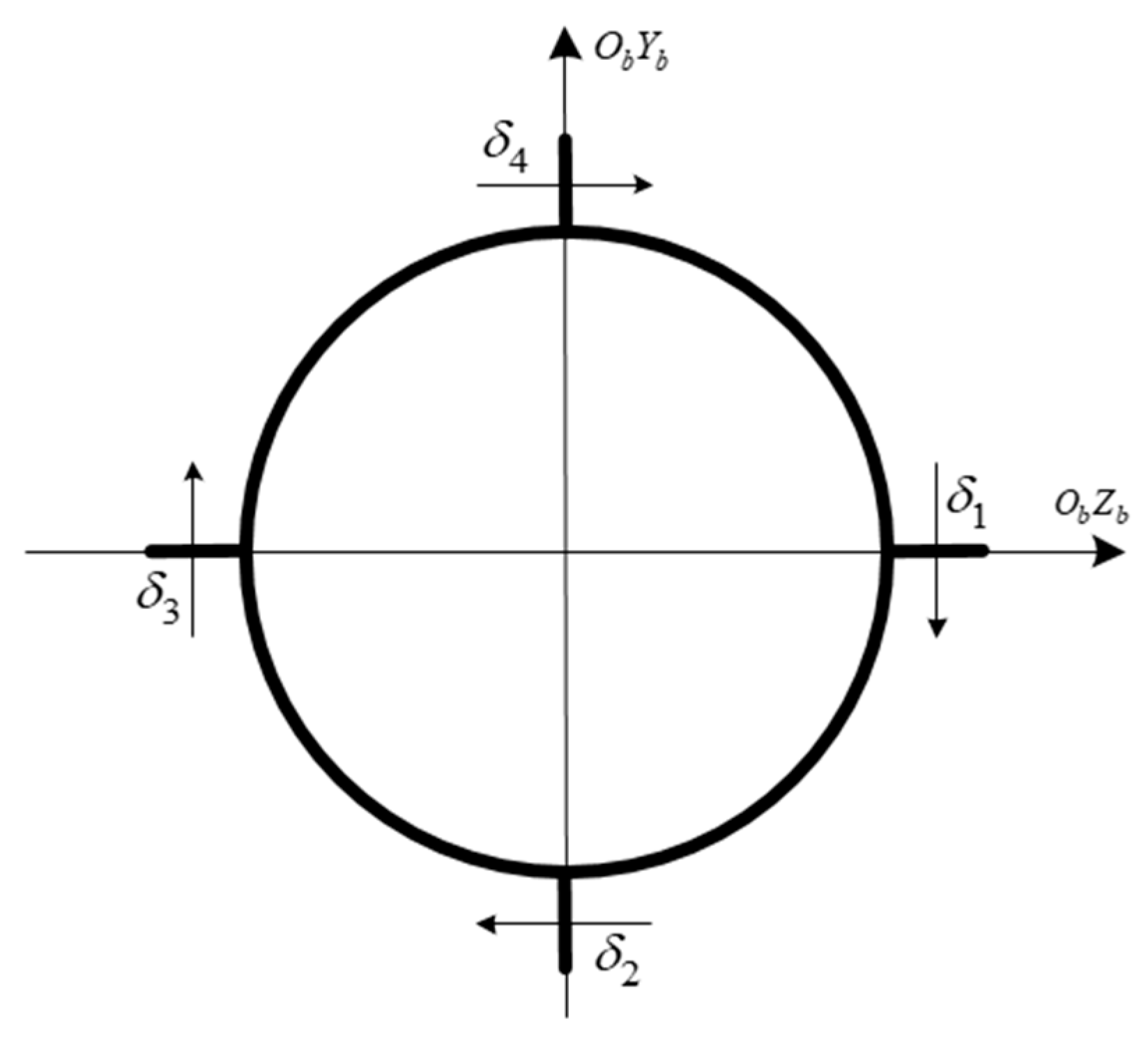
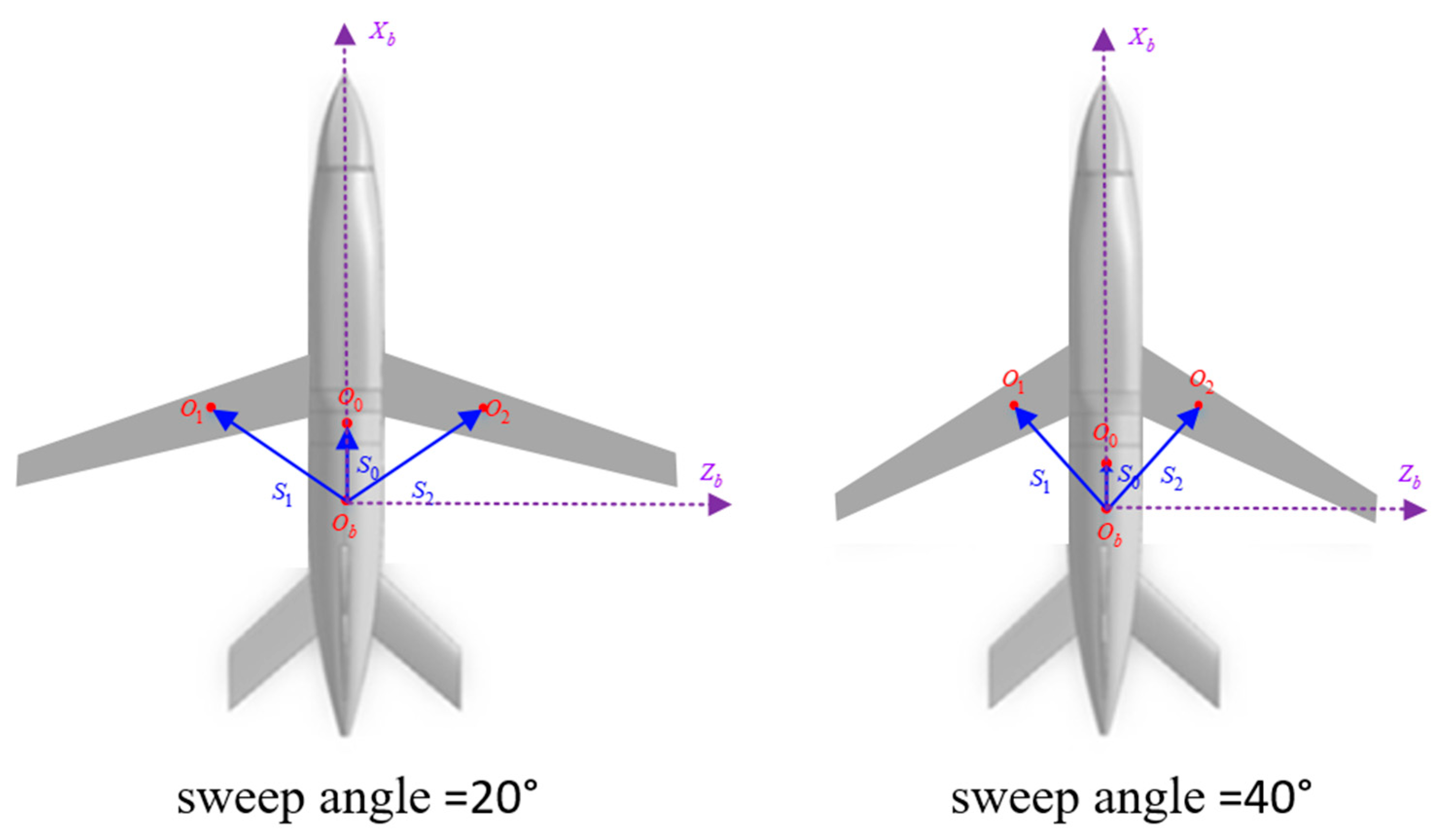
The subject of this paper is a variable swept angle morphing aircraft. Its swept-back angle can vary from 20° to 40° (Figure 1). The actuator of the aircraft is a group of cross rudders located in the tail section of the fuselage (Figure 2). The aircraft center-of-mass translational equation can be found in refs. [10,53]. The equation that describes the rotation of the morphing aircraft around the center of mass is shown below:
Ω ˙ = R ω J ω ˙ = ω × J ω + M 0 + B H δ r + Δ B H δ r + M S D + M S G + d
where Ω = ϕ , θ , ψ T represents the vector of Euler angles, ω = p , q , r T denotes the vector of angular rates, J is inertia matrix, δ r = δ r 1 , δ r 2 , δ r 3 , δ r 4 T is the control input vector, and M 0 represents the airframe-generated aerodynamic moment. d denotes disturbance vector. M S D and M S G denotes the additional moments arising from airfoil deformation and shifts in the aircraft’s center of mass; the expressions for R , J , ω × , H , M 0 and B are as follows:
R = 1 tan θ sin ϕ tan θ cos ϕ 0 cos ϕ sin ϕ 0 sin ϕ / cos θ cos ϕ / cos θ
J = J x x J x z 0 J x z J z z 0 0 0 J y y
ω × = 0 r q r 0 p q p 0
H = 1 4 1 1 1 1 2 0 2 0 0 2 0 2
M 0 = Q S r e f L m x 0 m z 0 m y 0
B = Q S r e f L m 0 x δ x 0 0 0 m 0 z δ z 0 0 0 m 0 y δ y
Δ B = Q S r e f L Δ m 0 x δ x 0 0 0 Δ m 0 z δ z 0 0 0 Δ m 0 y δ y
where S r e f , L , Q denote pneumatic reference area, pneumatic reference length and the dynamic pressure, respectively. m j 0 , m 0 j δ j , Δ m 0 j δ j denotes fuselage moment coefficient, aerodynamic multi-moment coefficient and aerodynamic multi-moment coefficient deviation, respectively.
Assumption 1 [54].
The centers of mass for both the fuselage and the wings are located within the   X b O b Z b  plane, and the two wings are identical.
Based on Assumption 1 and the multigrid body model in ref. [53], M S D and M S G can be written as follows:
M S D = 2 p J ˙ 1 x ( p ˙ + q r ) J 1 x m 1 S 1 x ( w ˙ + v p μ q ) q J ˙ 1 y + ( p r q ˙ ) J 1 y m 1 S 1 x ( v ˙ + μ r w p ) r J ˙ 1 x + J ˙ 1 y r ˙ J 1 x + J 1 y p q J 1 y J 1 x
M S G = 0 S 0 x m 0 + 2 S 1 x m 1 g cos φ cos γ S 0 x m 0 + 2 S 1 x m 1 g cos φ sin γ
The definition of each variable can be found in ref. [55].

2.2. Control-Oriented Model of the Morphing Aircraft

Based on Equation (1) the control state equation can be written as
x ˙ 1 = R x 2 x ˙ 2 = f + J 1 B δ + D
where x 1 = Ω , x 2 = ω , f = J 1 ω × J ω + J 1 M 0 , δ = δ x , δ z , δ y T = H δ r is the equivalent rudder deflection vector, and D = J 1 d + Δ B δ + M S D + M S G denotes the total perturbation, encompassing the sum of multiple unknown disturbances experienced by the aircraft during deformable maneuvers, including state deviations, aerodynamic uncertainties, and additional deformational disturbances.
Remark 1.
Equation (1) indicates that, unlike conventional fixed-shape aircraft, the morphing aircraft’s dynamics model includes additional moment terms  M S D  and  M S G  that are associated with the flight state. Combined with the expression for the deformed additional perturbation in Equations (9) and (10), it is known that if the aircraft attitude angular velocity is too large during the morphing maneuver, it will significantly enhance the value of the deformation additive perturbation, which in turn affects the control quality. Therefore, constraints must be imposed on the flight state to mitigate the additional perturbations from deformation. This represents a distinctive feature of the morphing aircraft and is a crucial consideration in the design of its controller.
Thus, control errors must be limited in order to obtain more stable flight performance and avoid larger deformation moments from larger system states leading to vehicle destabilization:
e 1 j Ω 1 j = e 1 j R : b _ 1 j < e 1 j < b ¯ 1 j , j = 1 , 2 , 3 e 2 j Ω 2 j = e 2 j R : b _ 2 j < e 2 j < b ¯ 2 j , j = 1 , 2 , 3
where b _ 1 j , b ¯ 1 j , b _ 2 j , b ¯ 2 j are changeable boundaries and where e 1 = x 1 x d , e 2 = x 2 x 2 r denote the system state errors. x d denotes the guidance command, and x 2 r indicates the actual virtual control quantity of the filter output.
Assumption 2 [5,56].
The initial state error satisfies the constraint, i.e.,  e 1 j ( 0 ) Ω 1 j , e 2 j ( 0 ) Ω 2 j .
Remark 2.
Typical forms of boundary changes can be summarized as:  b = ρ ( t ) , where  ρ ( t )  is a monotonically decreasing function, e.g.,  ρ ( t ) = ρ 0 e k ρ t + ρ  [57],  ρ ( t ) = 1 k ρ 1 t + 1 / ρ 0 + ρ  [58]. Nonetheless, the aforementioned function is typically designed to converge to a small steady-state value, thereby robustly ensuring the tracking performance. However, since the morphing aircraft may experience a sudden mission change or strong maneuvering breakout process during flight, a widespread sudden change in guidance commands could result. Additionally, if the morphing aircraft is subjected to a transient strong perturbation effect during flight, this could result in a sharp increase in the state of the system. All of these factors can cause the system state error to touch the small and unchanging steady-state boundary easily, which triggers the singularity problem, leading to severe saturation of the actuator and the system state eventually exceeding the set boundary.
For this purpose, we design the following improved form of the boundary function:
b ¯ ( t ) = ρ ¯ ( t ) + ρ a ( t ) b _ ( t ) = ρ _ ( t ) + ρ a ( t ) ρ a ( t ) = k ρ 1 x ˙ d 2 + k ρ 2 2 b ¯ ( t τ ) e ( t ) cos 2 π b ¯ ( t τ ) b ¯ ( t τ ) e ( t ) + k ρ 2 2 b ¯ ( t τ ) e ( t ) 0.5 b ¯ ( t τ ) e ( t ) < b ¯ ( t τ )   a n d   t > T c 0.5 cos 2 π 0.6 b ¯ ( t τ ) e ( t ) + π 3 + 0.5 k ρ 1 x ˙ d 2 0.2 b ¯ ( t τ ) e ( t ) < 0.5 b ¯ ( t τ )   a n d   t > T c k ρ 1 x ˙ d 2 + k ρ 2 2 b _ ( t τ ) e ( t ) cos 2 π b ¯ ( t τ ) b _ ( t τ ) e ( t ) + k ρ 2 2 b _ ( t τ ) e ( t ) 0.5 b _ ( t τ ) e ( t ) > b _ ( t τ )   a n d   t > T c 0.5 cos 2 π 0.6 b _ ( t τ ) e ( t ) + π 3 + 0.5 k ρ 1 x ˙ d 2 0.2 b _ ( t τ ) e ( t ) > 0.5 b ( t τ )   a n d   t > T c 0 0.2 b ¯ ( t τ ) < e ( t ) < 0.2 b ¯ ( t τ )   o r   t T c
Remark 3.
According to Equation (13), the constraint boundary comprises two principal components: the prescribed performance boundary  ρ ( t )  ( ρ ¯ ( t )  and  ρ _ ( t )  represent the upper and lower bound functions of the conventional preset performance method, respectively.) and the adaptive adjustment boundary  ρ a ( t ) .  τ  denotes the simulation step size. The prescribed performance boundary is designed with the mission’s control performance requirements and the objectives of mitigating additional interference from deformation serving as its reference basis. The adaptive adjustment boundary is determined by the rate of command change, system error, and the deviation from constraint boundary. The constraint boundaries are smooth and continuous around each threshold, so the derivative singularity problem does not arise. Notably, the gains  k ρ 1  and  k ρ 2  should be designed considering the structural constraints of the aircraft and the maximum system state deviation limit that can complete the maneuvering flight.

2.3. Control Objective

According to the above analysis, compared with traditional fixed-form aircraft, morphing aircraft, owing to their structure, shape and flight state, have undergone significant changes that have a greater impact on their aerodynamic and mass characteristics; thus, the morphing aircraft model has stronger coupling and time-varying characteristics. In addition, the unpredictable changes in the flow field during the deformation process and the effects of additional deformation disturbances lead to greater uncertainties in the morphing aircraft model. This poses significant challenges when designing attitude control systems for morphing aircraft.
The objective of this paper is to design an appointed-time controller that can adaptively adjust the constraint boundaries according to the flight state so that the attitude tracking error of morphing aircraft can always satisfy the constraints during the morphing maneuver and that the convergence time can be accurately regulated with low conservatism.

3. Controller Design

To complete the appointed-time control of the morphing aircraft with constraints, several important definitions and lemmas related to controller design are introduced in Section 3.1. Then, an error transformation method is proposed in Section 3.2 to transform the constrained control model to an equivalent unconstrained control model. Furthermore, to address the issue of ‘differential explosion’, Section 3.3 details the design of an adaptive appointed-time filter. Finally, Section 3.4 designs the appointed-time control law and analyzes the stability of the closed-loop system.

3.1. Preliminaries

For the following system:
x ˙ = f x t , d ( t ) ,               x 0 = x 0 n , x n
where x is the system state variable, f is a continuous nonlinear function on n , d denotes an unknown bounded perturbation that varies with time.
Assumption 3.
The guidance command  x d  is always satisfied with  x d j Ω 1 j , while  x d  and  x ˙ d  are continuous and satisfy  x d 2 + x ˙ d 2 + x ¨ d 2 X D , where  X D  is a positive constant.
Definition 1 [59].
If system (14) is asymptotically stable, then for all  t > T ( x 0 ) , where  T ( x 0 )  denotes a function expression associated with the initial state variable. Its state variable  x  remains bounded. Then, system (14) is finite-time stable.
Definition 2 [59].
The system (14) is fixed-time stable if it is finite-time stable and  T ( x 0 )  is bounded (i.e.,  x 0 n : T x 0 T max ).
Definition 3 [60].
If for any positive constant  T c ,  x t  remains bounded for all  t T c , where  T c  is called the predefined time, and the origin of system (14) is predefined-time stable.
Definition 4 [33].
If system (14) is predefined-time stable, the actual convergence time  t c  of system (14) satisfies  T c = t c . Then, the origin of system (14) is appointed-time stable.
Remark 4.
For finite-time stability, the expected convergence time depends on the initial state error, making it impossible to accurately estimate its magnitude. For fixed-time stability, while the expected convergence time is independent of the initial state error, the numerous control parameters determining it and their complex expressions make presetting these parameters challenging. Predefined-time stability can express the expected convergence time with just one control parameter. However, due to multiple scaling operations during its derivation, the expected convergence time differs significantly from the actual convergence time. Therefore, the appointed-time method proposed in this paper aims to resolve all issues in the aforementioned stability control methods: it enables the expected convergence time to be independent of the initial state error and represented by a single control parameter, while also reducing the conservatism between the expected convergence time and the actual convergence time.
Lemma 1.
For system (14), which is actually appointed-time stable, if exists a continuous positive Lyapunov function  V x : R n R + 0 , it satisfies:
V ˙ α V + κ ˙ ( t ) κ ( t ) V + ξ κ ( t ) = ( 6 t 2 + 3 t T c + T c 2 ) ( T c t ) 3 T c 5 + ϖ 0 t < T c ϖ t T c
where  α  is a positive constant,  0 < ϖ 1 ,  T c > 0  is an appointed-time parameter, and  ξ  is a small positive constant.
Proofs: 
The derivation of the variable V ( t ) / κ ( t )  yields
d d t V κ = V ˙ κ κ ˙ κ 2 V
Bringing Equation (15) into the preceding equation yields
d d t V κ α V κ + ξ κ
Integrating both sides of Equation (17):
V κ e α t V ( 0 ) 1 + ϖ + ξ α κ
Continuing to simplify, we have
V e α t V ( 0 ) κ 1 + ϖ + ξ α
According to Equation (19), it follows that
lim t T c V ϖ e α T c V ( 0 ) + ξ α
Therefore, one can see that the state variables of the system (14) converge to a neighborhood near the origin Ω = x | V ( x ) ϖ e α T c V ( 0 ) + ξ α within an appointed time T c and always remain in that neighborhood for t T c , i.e., the system (14) is practically appointed-time stable. □
Remark 5.
Regarding the appointed-time method described in this paper, it can be seen from the proof of Lemma 1 that scaling operations were performed only in the first step (i.e., from Equation (16) to Equation (17)): by applying the standard form for appointed-time (Equation (15)),  V ˙  was scaled to  α V + κ ˙ ( t ) κ ( t ) V + ξ . In the subsequent integration steps, no scaling operations were ever performed on the right-hand side of the inequality. Furthermore, in the final convergence region, since  ϖ  is a small number that can be chosen arbitrarily, it can be set to  ϖ = 1 V 0  to ensure that the convergence region is independent of the initial state; consequently, the system will converge exactly to  Ω = x | V ( x ) e α T c + ξ α  at the specified convergence time  T c . In theory, if  V ˙ = α V + κ ˙ ( t ) κ ( t ) V + ξ  holds true at all times, the actual convergence time of the system to a neighborhood of the origin  Ω  will be exactly equal to the expected convergence time.
However, for predefined-time methods in ref. [61], if the standard form of the predefined-time stability proof is V ˙ ( x ) π η T c α β α V 1 η 2 + β V 1 + η 2 + ϵ , then during the first step of the procedure (i.e., Equation (12) in the paper), dV must be scaled. Furthermore, before arriving at Equation (14), the assumption that 2 η α β arctan β α V x 0 η 2 = π η α β implies a significant scaling of V ( x 0 ) in this step, resulting in the estimated convergence time being highly conservative. In contrast, the appointed-time designed in this paper does not suffer from the aforementioned issues; consequently, the convergence time predicted by the method proposed in this paper will be much closer to the actual convergence time.
Remark 6.
For  κ ( t ) , the expressions for its first and second-order derivatives are as follows:
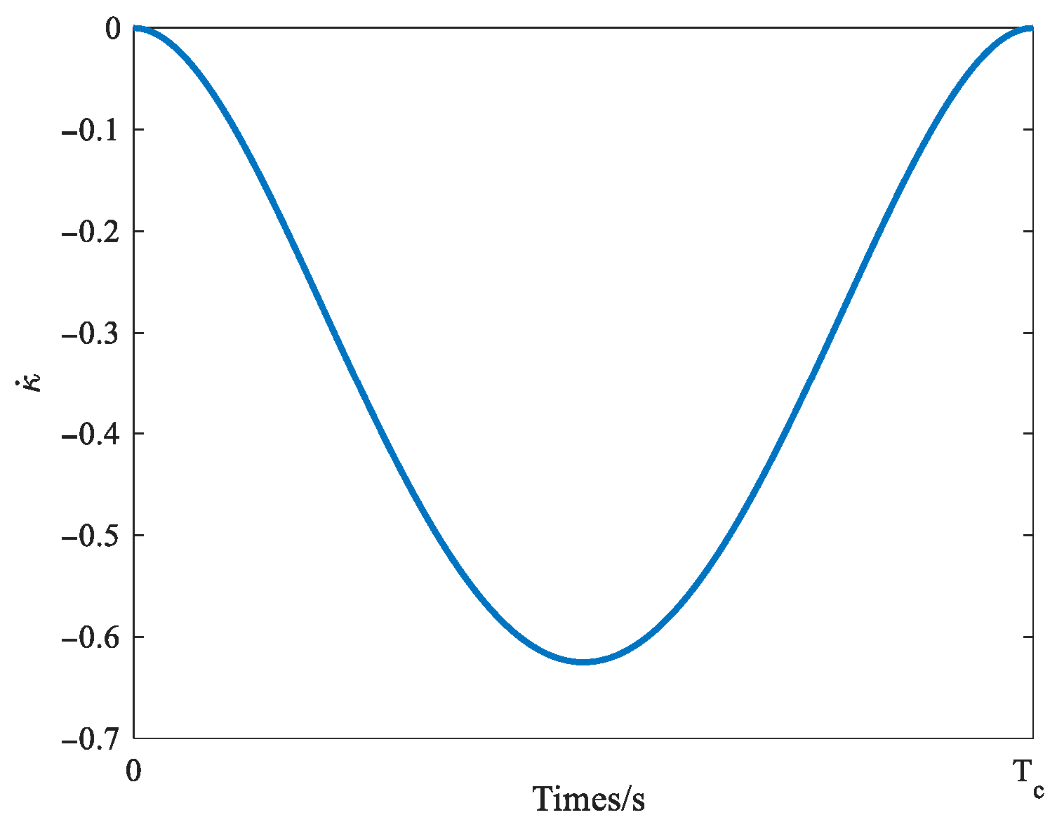
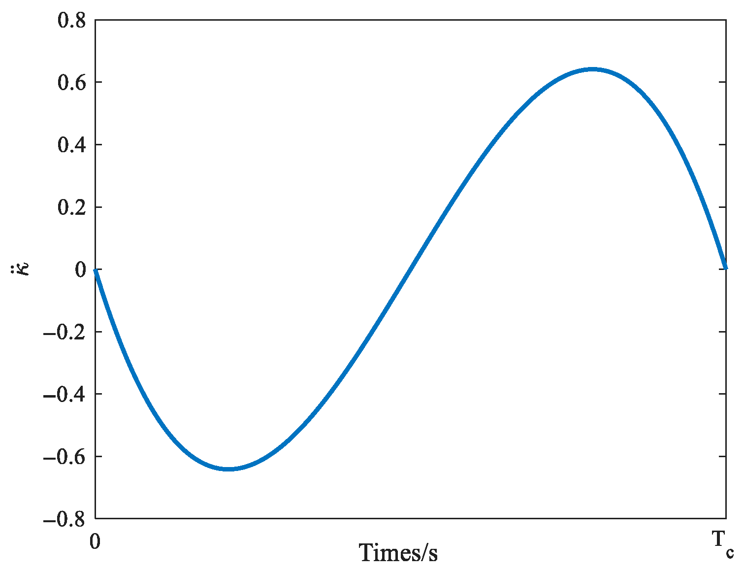
κ ˙ ( t ) = 30 t 2 ( T c t ) 2 T c 5 0 t < T c 0   t T c κ ¨ ( t ) = 60 t ( T c t ) ( T c 2 t ) T c 5 0 t < T c 0     t T c
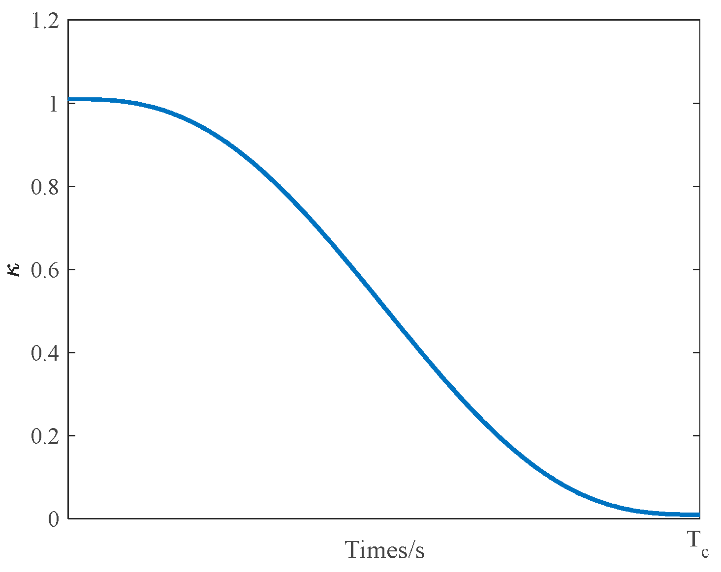
According to Equation (21) it can be seen that  lim t T c κ ˙ = lim t T c + κ ˙ = 0 and  lim t T c κ ¨ = lim t T c + κ ¨ = 0 . Therefore, the function κ ( t ) is smooth and continuous for t 0 , and because κ ˙ ( 0 ) = κ ¨ ( 0 ) = 0 (as shown in Figure 3, Figure 4 and Figure 5), compared with refs. [33,62], this method has a smaller control moment at the initial moment, which effectively prevents actuator saturation resulting from a large initial error.
Remark 7.
In classical terminal control [63,64], the convergence time can be adjusted via terminal constraints, and singularity issues can be addressed through methods such as coefficient freezing and terminal condition regularization. However, appointed-time stability is fundamentally different, as it requires the system to converge within a predetermined time independent of the initial conditions, and is based on Lyapunov feedback design rather than an optimal control framework. Therefore, this paper does not represent an extension of classical terminal control, but rather proposes a appointed-time stabilization method with an explicit time specification.

3.2. Control Model Transformation

To address the challenge of satisfying control performance constraints, this paper designs the following form of universal barrier transformation function (UBTF):
Λ i j = b _ i j e i j 2 ( b _ i j + e i j ) + b ¯ i j e i j 2 ( b ¯ i j e i j ) = A i j e i j , i = 1 , 2 , j = 1 , 2 , 3
where Λ i = Λ i 1 , Λ i 2 , Λ i 3 T , A i = d i a g ( A i 1 , A i 2 , A i 3 ) , and A i j = b _ i j 2 ( b _ i j + e i j ) + b ¯ i j 2 ( b ¯ i j e i j ) .
Remark 8.
According to Equation (22), if  e i j  approaches the boundary of  Ω i j ,  Λ i j  converges as follows:
lim e i j b _ i j Λ i j , lim e i j b ¯ i j Λ i j +
and if  b _ i j = b ¯ i j ,  Λ i j  is
lim b _ i j = b ¯ i j + Λ i j e i j
Thus, compared with the barrier transform in refs. [51,52,65], the barrier transform method described in this paper can be applied not only to asymmetric state error constraints but also to unconstrained control problems. Therefore, it is universal.
Applying the above transformation combined with Equation (11) yields the state error equation of the system under unconstrained conditions as
Λ ˙ 1 = B 1 R x 2 B 1 x ˙ d + C 1 Λ ˙ 2 = B 2 ( f + J 1 B δ + D x ˙ 2 r ) + C 2
where B i j = b _ i j 2 2 ( b _ i j + e i j ) 2 + b ¯ i j 2 2 ( b ¯ i j e i j ) 2 , C i j = b _ ˙ i j e i j 2 2 ( b _ i j + e i j ) 2 + b ¯ ˙ i j e i j 2 2 ( b ¯ i j e i j ) 2 , B i = d i a g B i 1 , B i 2 , B i 3 , C i = C i 1 ; C i 2 ; C i 3 , and x ˙ 2 r indicates the derivative of the actual virtual control quantity of the filter output.

3.3. Adaptive Appointed-Time Filter

To solve the complex differential explosion problem, this paper designs an adaptive appointed-time filter with the following form:
x ˙ 2 r = m 1 α 1 κ ˙ ( t ) 2 m 1 κ ( t ) z + m 1 χ ^ χ ^ ˙ = 2 m 2 α 2 κ ˙ ( t ) 2 m 2 κ ( t ) χ ^ m 2 z
where m 1 , m 2 , α 1 , α 2 are positive constants, z = x 2 r x 2 c , and x 2 c is the virtual control quantity. We assume that x ˙ 2 c is bounded and that x ˙ 2 c j χ j , where χ = [ χ 1 , χ 2 , χ 3 ] T , χ j > 0 is unknown. χ ^ is the estimate of χ , and χ ˜ = χ χ ^ .
Theorem 1.
For the adaptive appointed-time filter (26), the filter and estimation error are practically appointed-time stable.
Proofs: 
Select a Lyapunov function as follows:
V f = z T z 2 m 1 + χ ˜ T χ ˜ 2 m 2
Deriving Equation (27) and combining it with Equation (26) yields
V ˙ f = z T α 1 κ ˙ ( t ) 2 m 1 κ ( t ) z + z T χ ^ z T x ˙ 2 c + 2 χ ˜ T α 2 κ ˙ ( t ) 2 m 2 κ ( t ) χ ^ + χ ˜ T z         = z T α 1 κ ˙ ( t ) 2 m 1 κ ( t ) z + 2 χ ˜ T α 2 κ ˙ ( t ) 2 m 2 κ ( t ) χ ^ + z T χ z T x ˙ 2 c         α 1 κ ˙ ( t ) 2 m 1 κ ( t ) z 2 + 2 χ ˜ T α 2 κ ˙ ( t ) 2 m 2 κ ( t ) χ χ ˜ + 0.5 z 2 + 0.5 χ x ˙ 2 c 2         α 1 κ ˙ ( t ) 2 m 1 κ ( t ) 0.5 z 2 α 2 κ ˙ ( t ) 2 m 2 κ ( t ) χ ˜ 2 + α 2 κ ˙ ( t ) 2 m 2 κ ( t ) χ 2 + 0.5 χ x ˙ 2 c 2         α f V f + κ ˙ ( t ) κ ( t ) V f + Ξ f
where α f = min 2 m 1 α 1 m 1 , 2 m 2 α 2 , and Ξ f = α 2 κ ˙ ( t ) 2 m 2 κ ( t ) χ 2 + 0.5 χ x ˙ 2 c 2 . According to Lemma 1, the filter error z and the estimation error χ ˜ are practically appointed-time stable. □

3.4. Controller Design and Stability Analysis

To keep the state error within the desired control performance during maneuvering of the morphing aircraft and achieve appointed-time stability, using the equivalent unconstrained control error model (25), a controller is designed in two steps:
Step 1: For the first equation in Equation (25), combined with the definition of z , it can be reduced as
Λ ˙ 1 = B 1 R e 2 + z + x 2 c B 1 x ˙ d + C 1
Virtual control variables are devised as
x 2 c = R 1 B 1 1 B 1 x ˙ d C 1 α 3 κ ˙ ( t ) 2 κ ( t ) Λ 1 B 1 R 2 Λ 1 2 λ 1 2
where λ 1 , α 3 > 0 . For the Lyapunov function V 1 = Λ 1 T Λ 1 2 , the derivation of which is given by
V ˙ 1 = Λ 1 T B 1 R e 2 + z + x 2 c B 1 x ˙ d + C 1
Bringing Equation (30) into Equation (31) yields
V ˙ 1 = Λ 1 T α 3 κ ˙ ( t ) 2 κ ( t ) Λ 1 + Λ 1 T B 1 R e 2 + Λ 1 T B 1 R z Λ 1 T B 1 R 2 Λ 1 2 λ 1 2       α 3 κ ˙ ( t ) 2 κ ( t ) Λ 1 2 + Λ 1 T B 1 R A 2 1 Λ 2 + λ 1 2 z 2 2
Step 2: Radial basis function (RBF) networks can approximate nonlinear functions with arbitrary accuracy on tight sets [15]. For this reason, this paper uses an RBF neural network to approximate for the total uncertainty perturbation, which is given by
D = W T ϕ ( x ) + ε
where W is the ideal weight of the network, ε is the bounded estimation error of the network to the perturbation, and ϕ ( ) is the Gaussian basis function. The input options for the neural network are x = [ x 1 , x 2 ] T . The output D ^ is the estimate of D .
D ^ = W ^ T ϕ ( x )
where W ^ is the estimation of W . We define Θ = W ^ 2 and Θ ˜ = Θ Θ ^ , where Θ ^ is the estimate of Θ , and its expression is as follows:
Θ ^ ˙ = 2 m 3 α 4 κ ˙ ( t ) 2 m 3 κ ( t ) Θ ^ + m 3 Λ 2 2 B 2 2 ϕ T ϕ 2 λ 2 2
where m 3 , λ 2 , α 4 are positive constants.
The control law is given as
δ = B 1 J f Θ ^ T ϕ 2 ( x ) Λ 2 2 λ 2 2 + x ˙ 2 r B 2 1 α 5 κ ˙ ( t ) 2 κ ( t ) Λ 2 B 1 J B 2 1 C 2       B 1 J B 2 1 A 2 1 T B 1 R T Λ 1 B 1 J B 2 1 B 2 2 Λ 2 2 λ 3 2
where λ 3 , α 5 are positive constants.
Theorem 2.
For the morphing aircraft dynamics model (11), if its initial value satisfies Equation (12), the closed-loop system (25) performs the following characteristics under the action of the adaptive appointed-time filter (26), the RBF neural network (34), (35) and the control inputs of Equations (30) and (36).
(1) e 1 , e 2 are practically prescribed-time stable and satisfy the constraints of Equation (12) all the time;
(2) All of the signal variables are practically appointed-time stable.
Proofs: 
Select the Lyapunov function as
V 2 = V 1 + V f + Λ 2 T Λ 2 2 + Θ ˜ 2 2 m 3
The derivation of the above equation yields
V ˙ 2 = Λ 1 T α 3 κ ˙ ( t ) 2 κ ( t ) Λ 1 + Λ 1 T B 1 R A 2 1 Λ 2 + Λ 1 T B 1 R z Λ 1 T B 1 R 2 Λ 1 2 λ 1 2     + z T α 1 κ ˙ ( t ) 2 m 1 κ ( t ) z + z T χ ^ z T x ˙ 2 c + 2 χ ˜ T α 2 κ ˙ ( t ) 2 m 2 κ ( t ) χ ^ + χ ˜ T z     Λ 2 T α 5 κ ˙ ( t ) 2 κ ( t ) Λ 2 Λ 2 T B 2 2 Λ 2 2 λ 3 2 Λ 2 T A 2 1 T B 1 R T Λ 1     + Λ 2 T B 2 ε + W ϕ Λ 2 T B 2 Θ ^ T ϕ 2 ( x ) Λ 2 2 λ 2 2 Θ ˜ Θ ^ ˙ m 3
Combining Equations (28), (32) and (35) to deflate Equation (38), we can obtain
V ˙ 2 α 1 κ ˙ ( t ) 2 m 1 κ ( t ) z 2 α 2 κ ˙ ( t ) 2 m 2 κ ( t ) χ ˜ 2 α 3 κ ˙ ( t ) 2 κ ( t ) Λ 1 2 α 5 κ ˙ ( t ) 2 κ ( t ) Λ 2 2   + α 2 κ ˙ ( t ) 2 m 2 κ ( t ) χ 2 + λ 1 2 z 2 2 Λ 2 T B 2 2 Λ 2 2 λ 3 2 + Λ 2 T B 2 ε + B 2 Λ 2 2 Θ ˜ ϕ T ϕ 2 λ 2 2 + λ 2 2 2   Θ ˜ 2 α 4 κ ˙ ( t ) 2 m 3 κ ( t ) Θ ^ + Λ 2 2 B 2 2 ϕ T ϕ 2 λ 2 2   α 1 κ ˙ ( t ) 2 m 1 κ ( t ) z 2 α 2 κ ˙ ( t ) 2 m 2 κ ( t ) χ ˜ 2 α 3 κ ˙ ( t ) 2 κ ( t ) Λ 1 2 α 5 κ ˙ ( t ) 2 κ ( t ) Λ 2 2   α 4 κ ˙ ( t ) 2 m 3 κ ( t ) Θ ˜ 2 + α 2 κ ˙ ( t ) 2 m 2 κ ( t ) χ + α 4 κ ˙ ( t ) 2 m 3 κ ( t ) Θ 2 + λ 1 2 z 2 2 + λ 2 2 2 + λ 3 2 ε 2 2   k V 2 + κ ˙ ( t ) κ ( t ) V 2 + Ξ
where the expressions for k and Ε are as follows:
k = min 2 m 1 ( α 1 λ 1 2 2 ) , 2 m 2 α 2 , 2 α 3 , 2 α 4 , 2 m 3 α 5 Ξ = α 2 κ ˙ ( t ) 2 m 2 κ ( t ) χ + α 4 κ ˙ ( t ) 2 m 3 κ ( t ) Θ 2 + λ 2 2 2 + λ 3 2 ε 2 2
According to Lemma 1, The inference can be made that the variables Λ 1 , Λ 2 , z , χ ˜ , Θ ˜ are practically appointed-time stable. Furthermore, combined with Equation (22), it can be deduced that since Λ 1 , Λ 2 are bounded at the appointed time T c , then e 1 , e 2 are also bounded at the appointed time T c and satisfy the constraints of Equation (12) all the time. Then, from Equations (30) and (36), we determine that x 2 c , δ are bounded. From this, we can infer that x 2 r , x 2 are also bounded. Additionally, since the control command x d is bounded, it follows that x 1 is bounded. Similarly, both χ ^ and Θ ^ are bounded. Therefore, all of the signal variables are practically appointed-time stable. □
Remark 9.
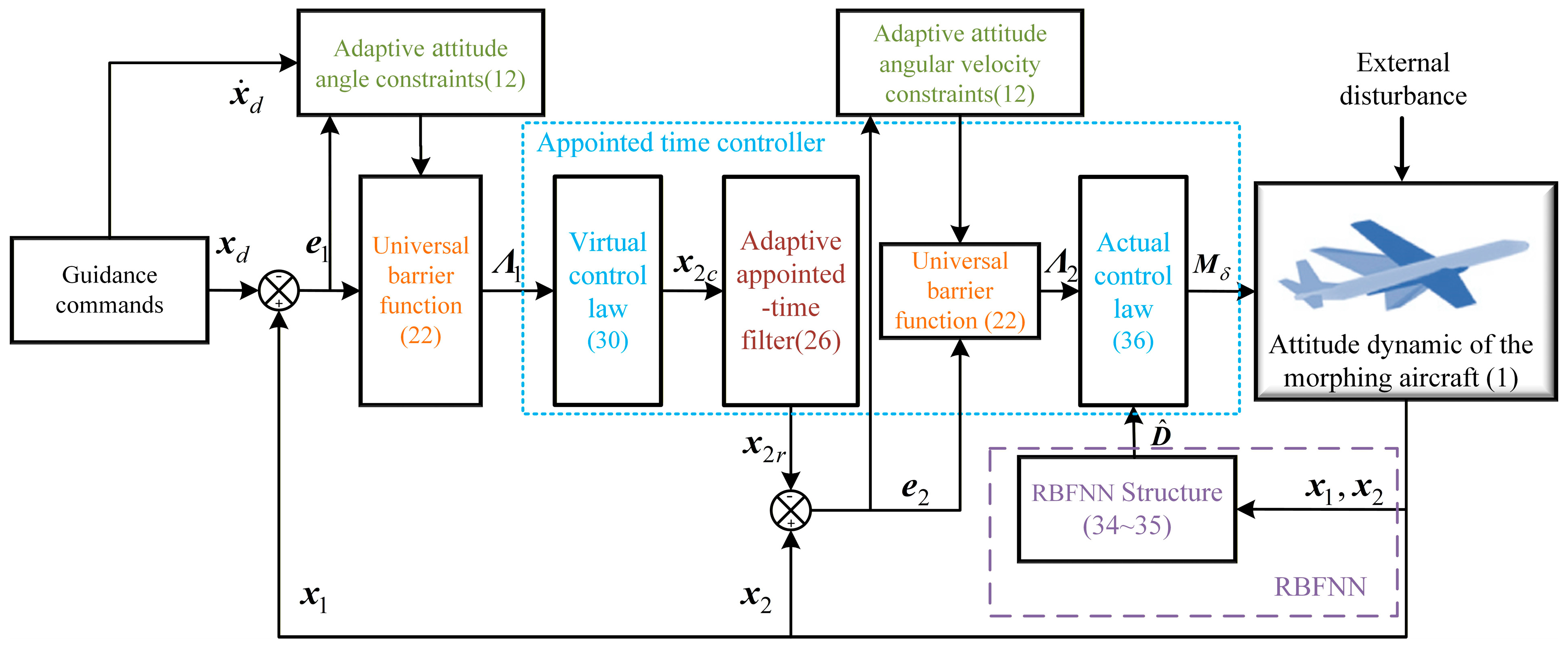
The controller structure is shown in Figure 6. This structure employs a UBTF (22) is used to ensure the system state error consistently remains within predefined constraints. Notably, the UBTF is applicable to both asymmetric and unconstrained constraint requirements without necessitating modifications to the control structure, thereby offering enhanced versatility. In addition, constraint function (4) can adaptively adjust the boundaries according to the flight state and command changes, thus avoiding the singularity problem of the traditional prescribed performance method when the system error approaches/exceeds the boundaries. The adaptive appointed time filter can effectively solve the differential explosion problem while ensuring appointed-time stability of the filtering error. Concurrently, the RBF neural network is employed to estimate unknown system disturbances. Finally, the appointed time controller ensures that all the signals of the closed-loop system can converge in the predesigned appointed time. This convergence time depends solely on a single control parameter and is independent of the initial state, significantly simplifying the parameter design process. Furthermore, the application of a time transformation function, whose initial first and second derivatives are zero, combined with the low conservatism of the convergence time, effectively prevents excessively large control commands during the initial response phase, which reduces the possibility of saturating the actuator.
Remark 10.
When selecting the control parameters,  α 1 ~ α 5  and  λ 1 ~ λ 3  affect the control accuracy at the time of convergence. A larger  α 1 ~ α 5  and a smaller  λ 1 ~ λ 3  can enhance control accuracy.  T c  mainly determines the convergence time, and  α 1 ~ α 5  also affects the convergence speed. A smaller  T c  and larger  α 1 ~ α 5  accelerate system convergence but also increase the likelihood of overshooting during the dynamic response.  k ρ 1  and  k ρ 2  denote the sensitivity of the performance boundary to the guidance command changing rate and the distance of the state error from the performance boundary, respectively. The larger  k ρ 1  and  k ρ 2  are, the more sensitive the performance boundaries are to the guidance command changing rate and the distance of the state error from the performance boundary, which can effectively avoid the singularity problem caused by state errors close to the boundaries; however, a value that is too large can also lead to the performance boundaries being overly relaxed, which can degrade the control quality or cause the maneuvering task not being completed. Therefore, selecting control parameters necessitates a careful trade-off, balancing these settings based on the system’s required control accuracy, actual response speed, and appointed performance boundary requirements.

4. Simulation Results

There are two sets of mathematical simulations performed in this section to demonstrate the feasibility and advantages of the proposed controller. Section 4.1 validates its appointed-time convergence characteristics. Subsequently, Section 4.2 conducts comparative simulations to evaluate its benefits for the attitude control performance of the morphing aircraft.

4.1. Effectiveness Verification

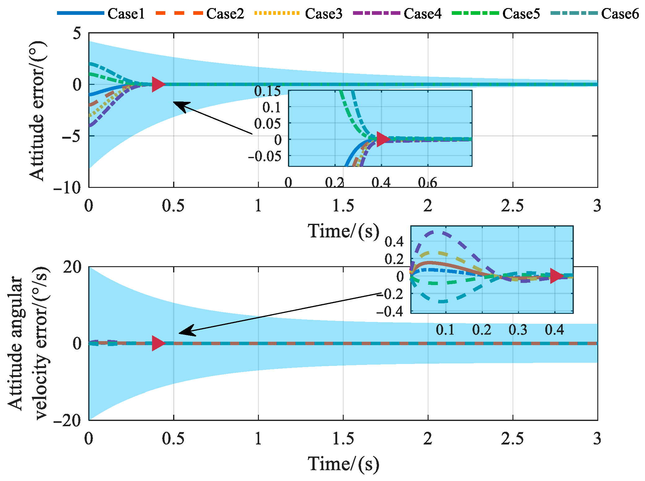
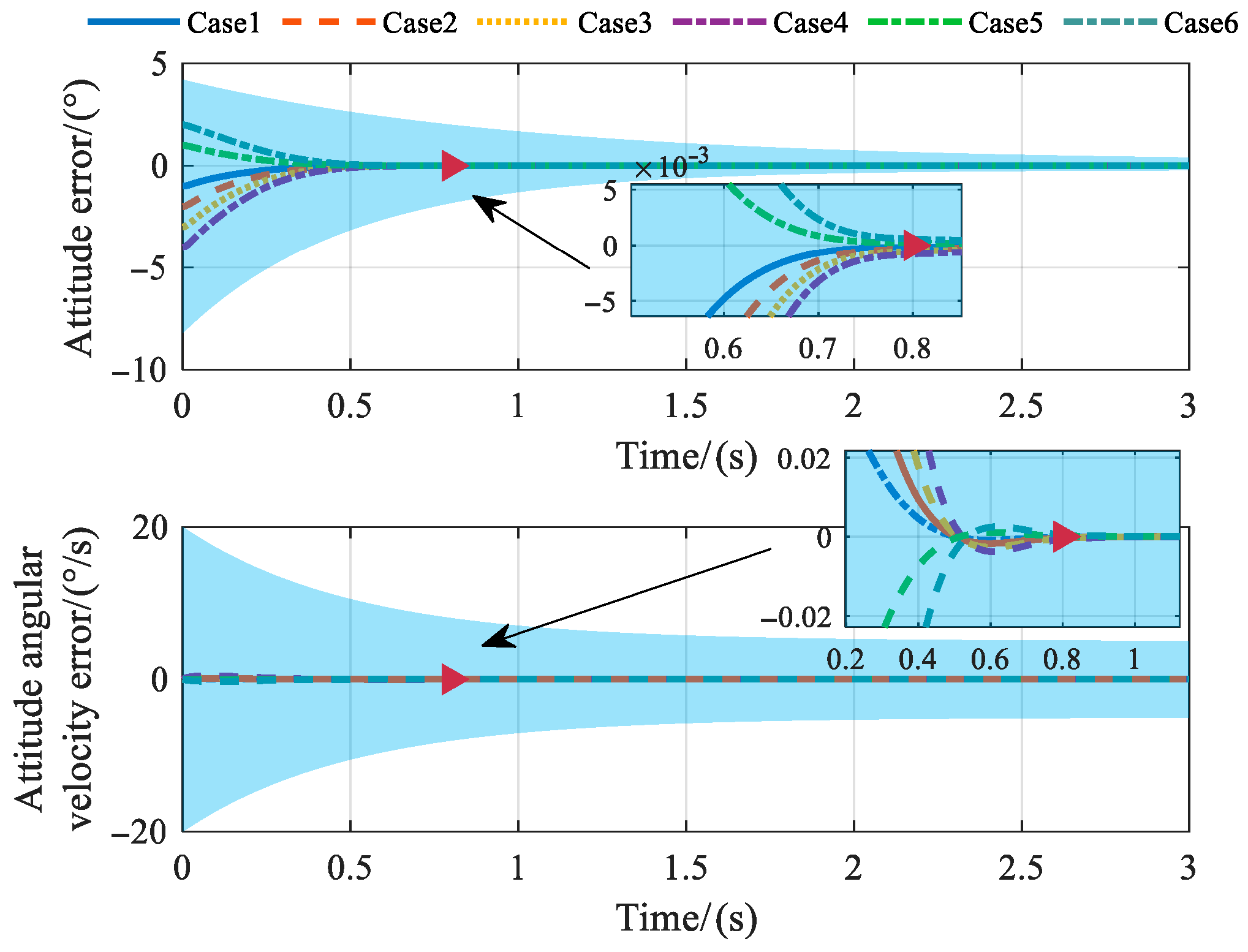
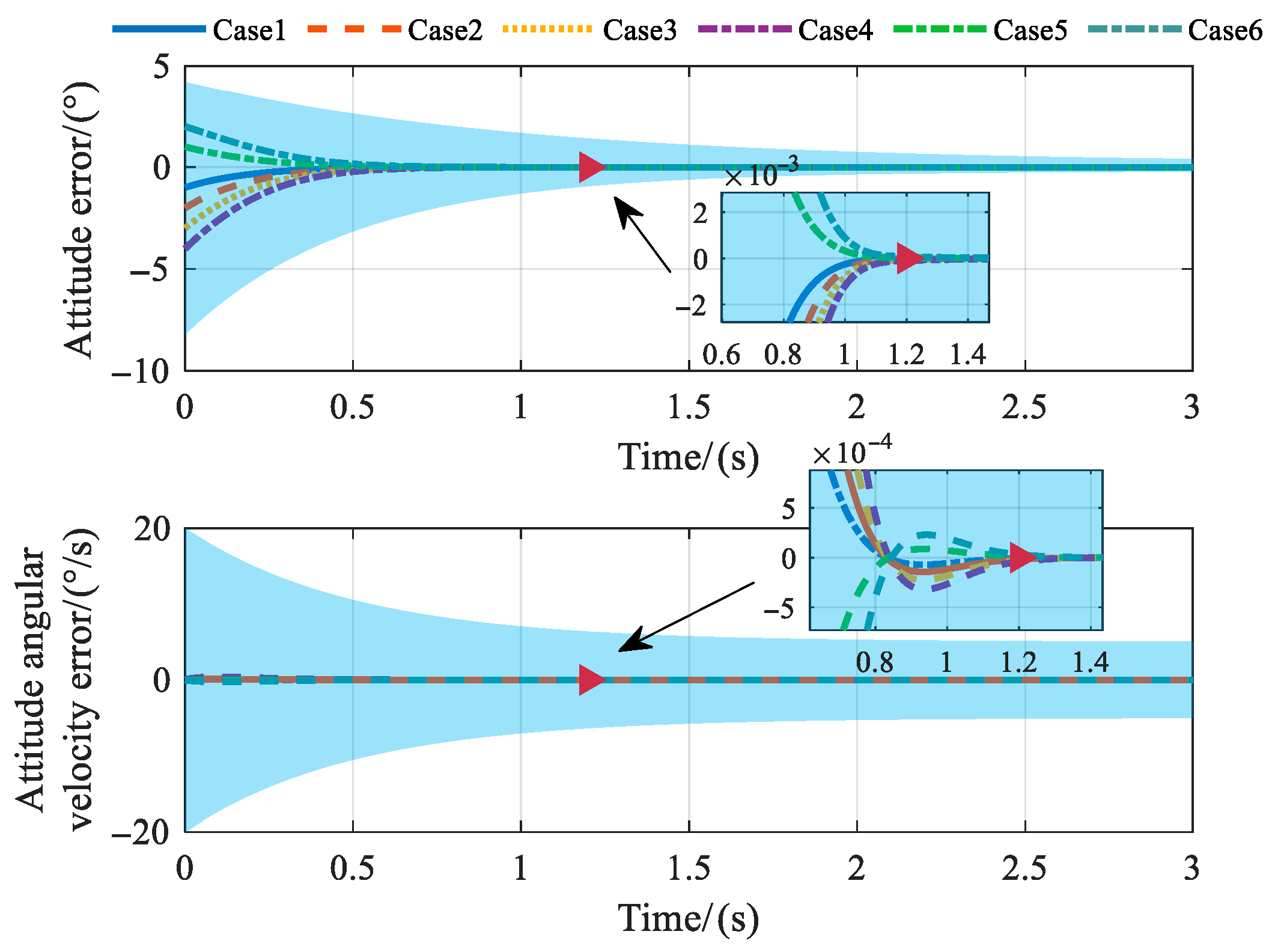
We use the φ -channel of the control-oriented model to verify the appointed-time convergence characteristics of the designed controller, and to ensure the comprehensiveness of the simulation, six initial states (as shown in Table 1) and three different convergence times ( T c = 0.4 , T c = 0.8 , T c = 1.2 ) are selected for demonstration to verify the following two features. The control parameters are shown in Table 2.
Feature 1.
For a given set of control parameters, the system’s convergence time does not depend on the initial conditions.
Feature 2.
The control parameter  T c  can precisely regulate the system’s convergence time.
The number of RBF neural network nodes is established as 30, and the initial weights are selected in a random range 1 , 1 .
The preceding simulation results in Figure 7, Figure 8 and Figure 9 demonstrate that the system state error converge to the vicinity of the origin within the appointed time T c , irrespective of their initial magnitudes. Furthermore, the actual convergence time can be precisely regulated by the control parameter T c .

4.2. Comparative Simulation

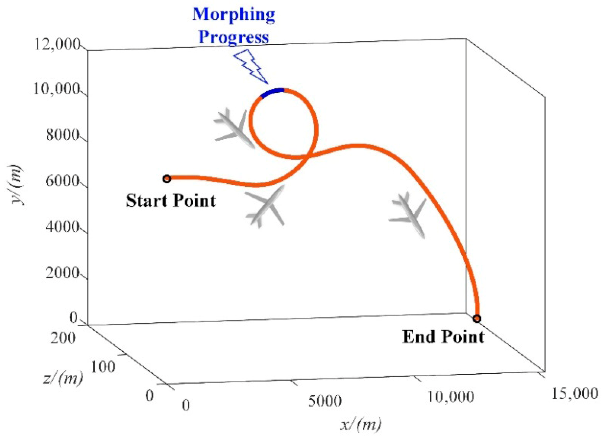
To validate advantages of the controller designed herein, this section presents a comparative analysis against two existing morphing aircraft control schemes. Controller 1 is a predefined-time controller designed in ref. [30], which does not consider the performance constraints, and Controller 2 is a prescribed-time controller provided in ref. [56], which accounts for the performance constraints, but the constraints cannot be adjusted adaptively. Similar to our previous study, a typical maneuvering trajectory (Figure 10) was selected to appraise the control quality. The aircraft’s back-sweep angle changes from 20° to 40° at 5°/s in the 15th second. The aerodynamic parameters are subjected to 20% uncertainty at the 30th second.
The initial conditions of the simulation are x 1 = 1 o , 1 o , 1 o ,   x 2 = 0 o / s , 0 o / s , 0 o / s , H 0 = 9000   m , and V 0 = 1000   m / s . The aerodynamic parameters of the aircraft and the external perturbation is the same as that in our previous research [55]. The overall structural parameters are shown in Table 3.
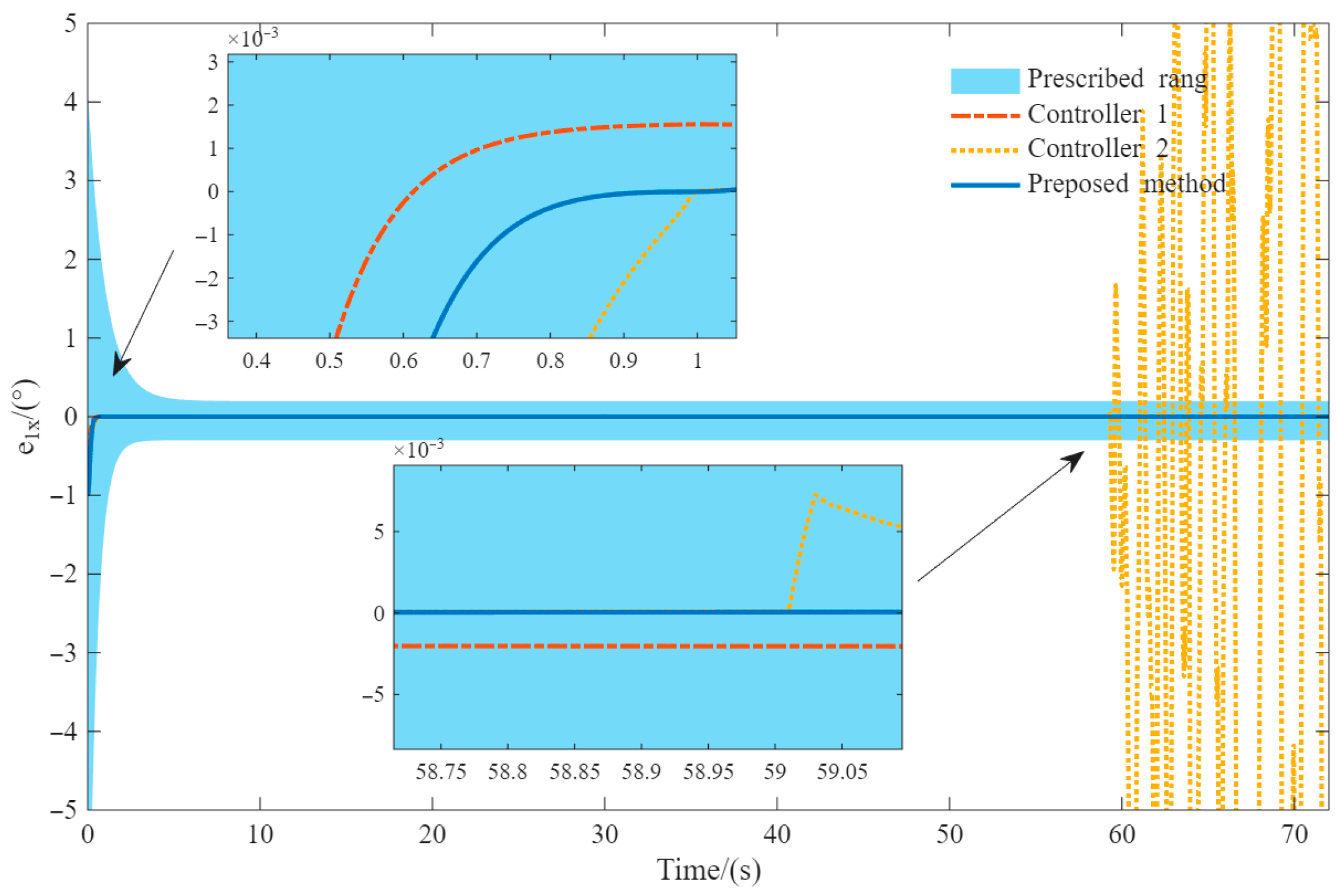
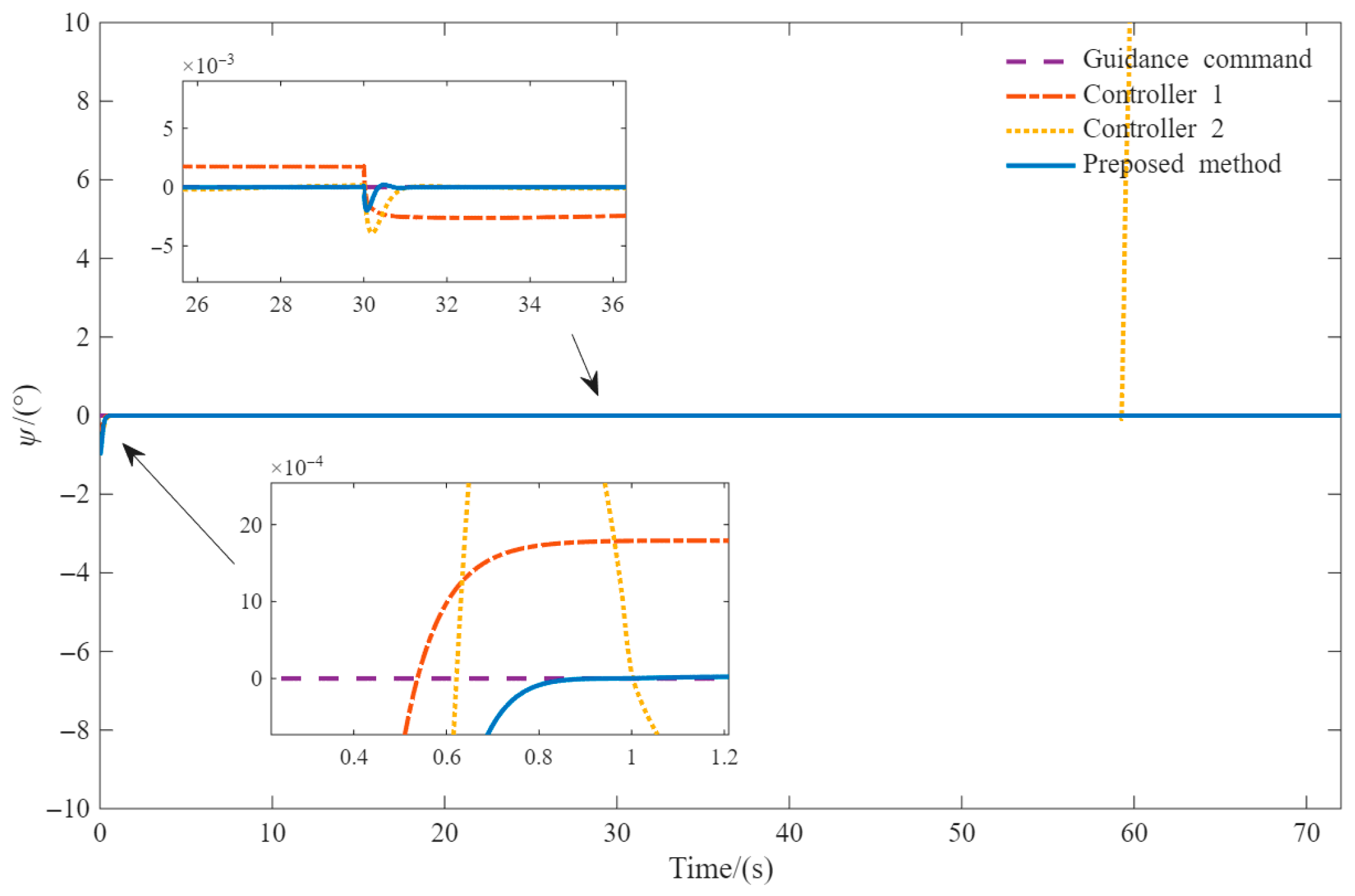
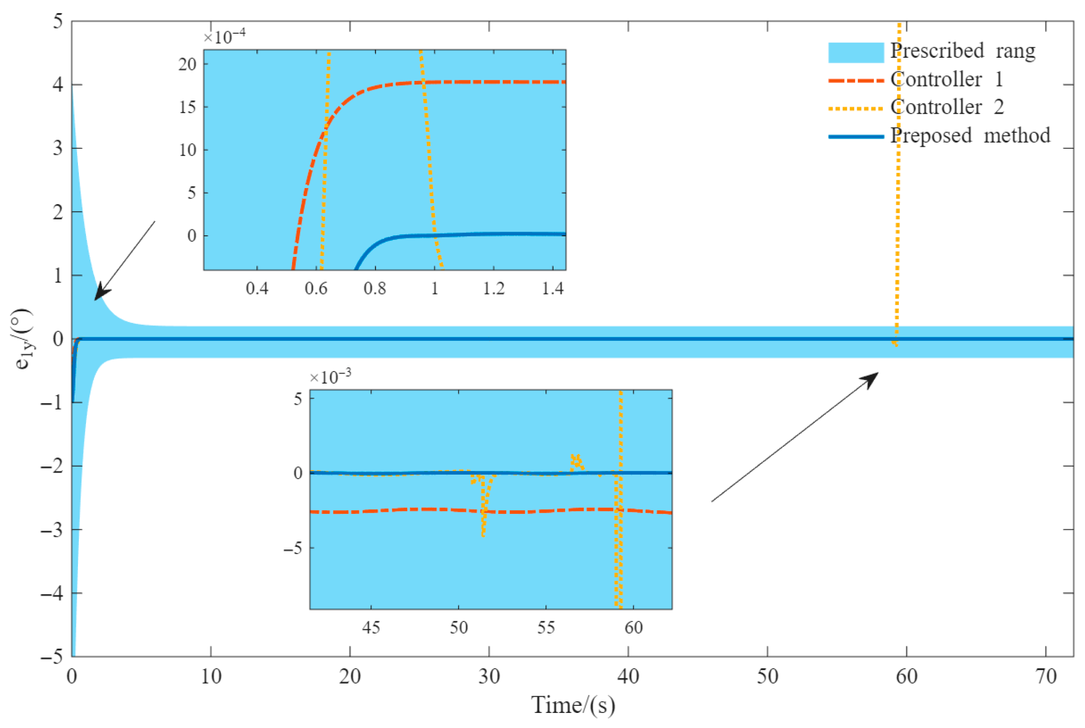
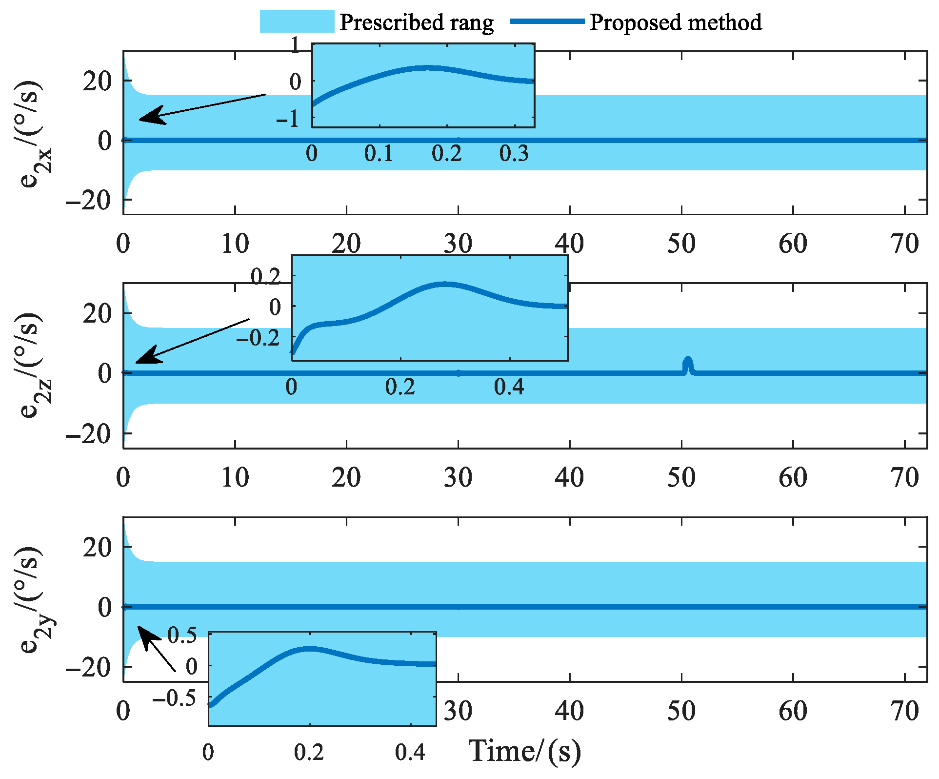
In addition, to ensure the fairness of the simulation, the convergence times and steady-state errors of the three methods were set to be close to each other in an undisturbed system. Simultaneously, while maintaining similar convergence times and steady-state errors, the control parameters of the three methods were further optimized to minimize overshoot during their dynamic response processes. The parameters of the controllers are shown in Table 4. The number of nodes is selected as N = 20, the centers are randomly chosen in [−1,1], and the width is set as 1. The simulation results are shown in Figure 11, Figure 12, Figure 13, Figure 14, Figure 15, Figure 16, Figure 17, Figure 18, Figure 19, Figure 20, Figure 21, Figure 22, Figure 23 and Figure 24.
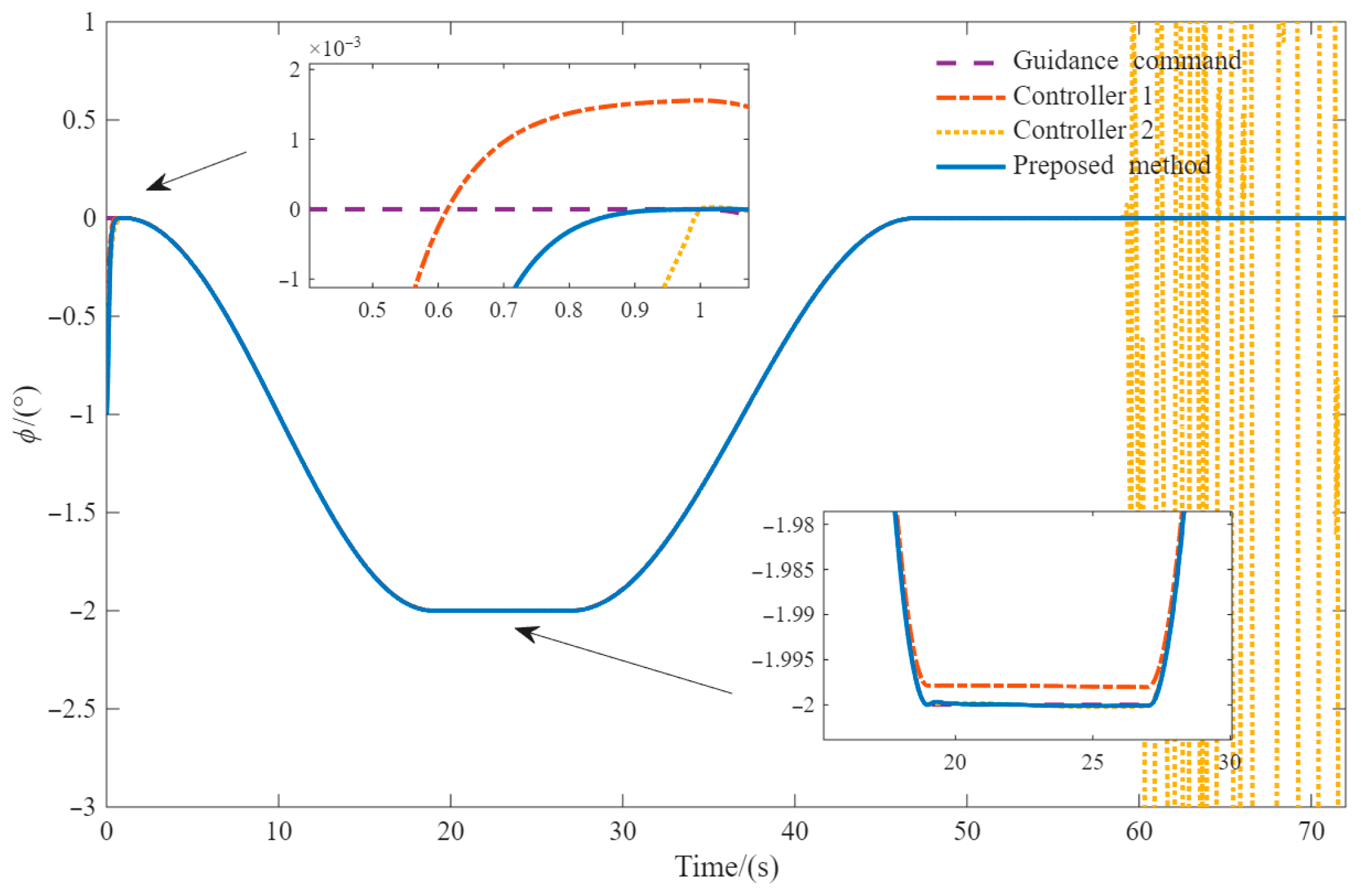
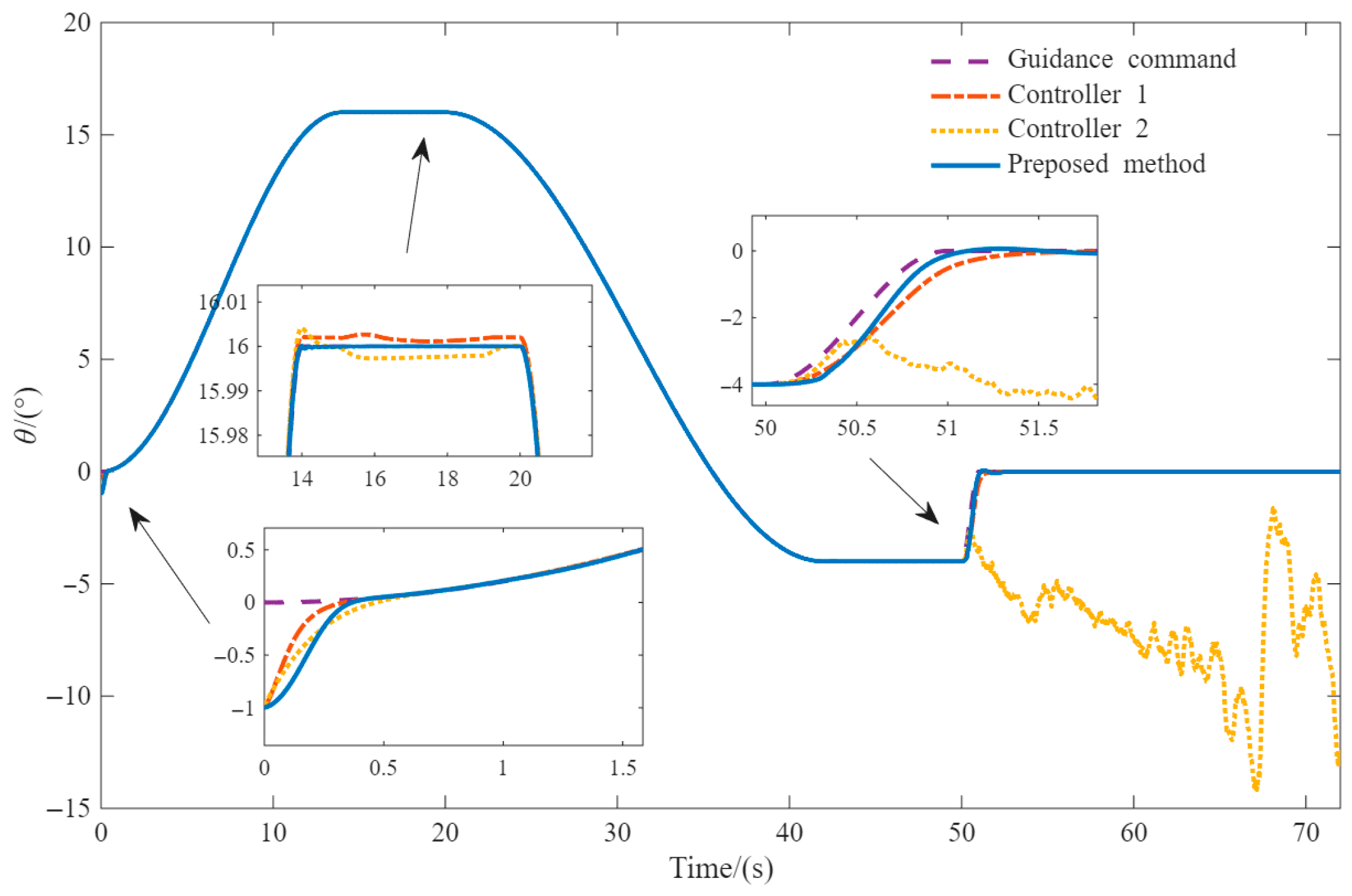
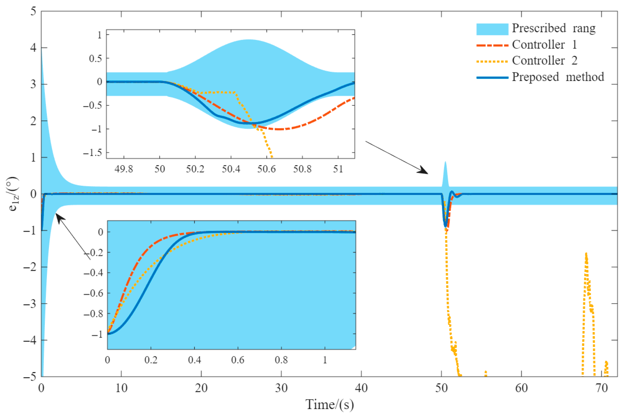
The three-channel attitude angles and attitude angle deviations under the action of different controllers are displayed in Figure 11, Figure 12, Figure 13, Figure 14, Figure 15 and Figure 16. These figures illustrate that this paper’s controller ensures the convergence of three-channel attitude angle errors within the appointed time, and exhibits significantly less conservatism compared to the other two methods. Moreover, when the aircraft encounters a rapidly changing command, the performance constraints are relaxed due to the adaptive boundary adjustment law (5). This prevents the singularity issues observed with Controller 2 when attitude errors approach or exceed the performance boundaries. Furthermore, the proposed method effectively addresses asymmetric performance constraint problems and demonstrates superior control accuracy compared to the other two controllers.
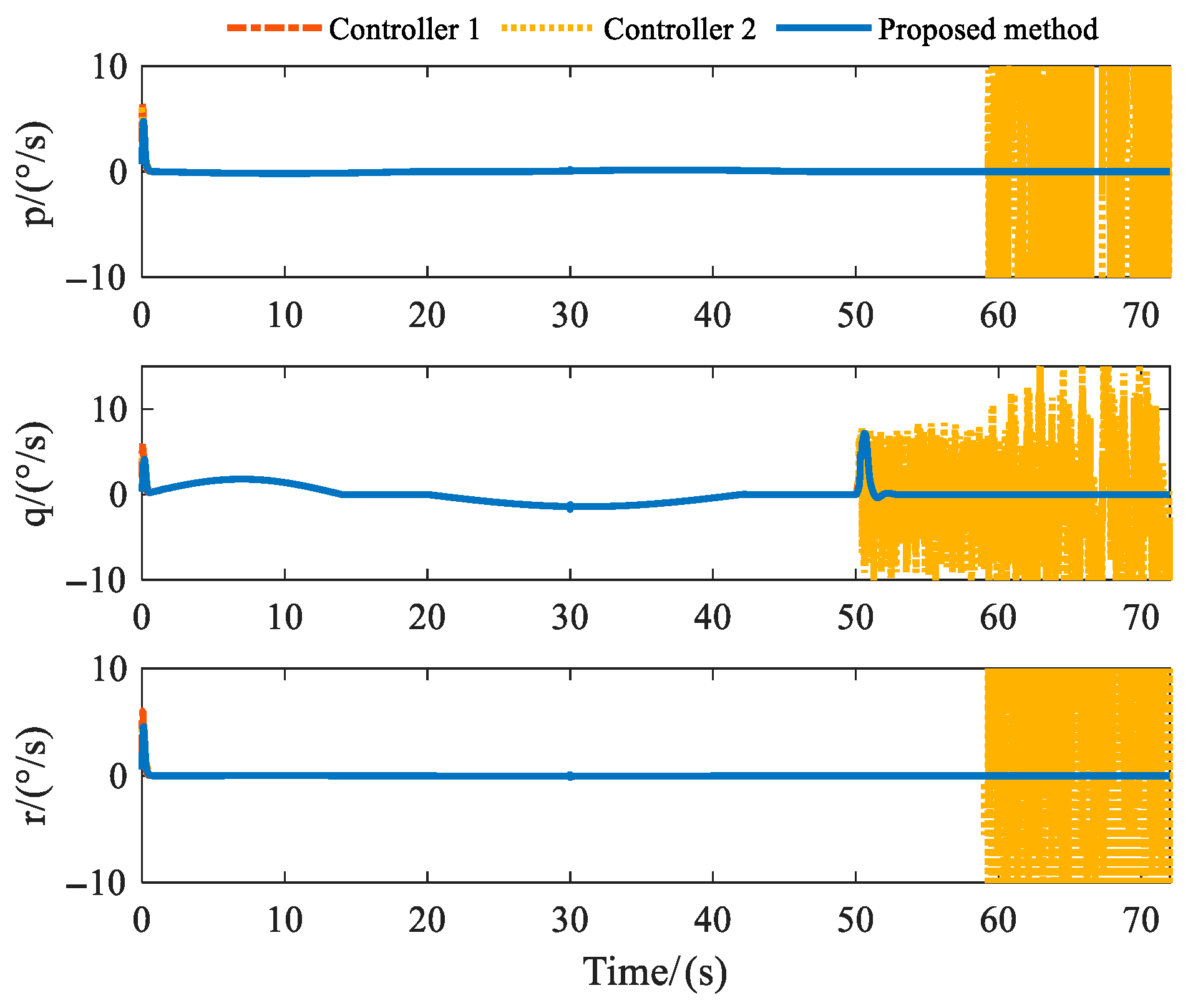
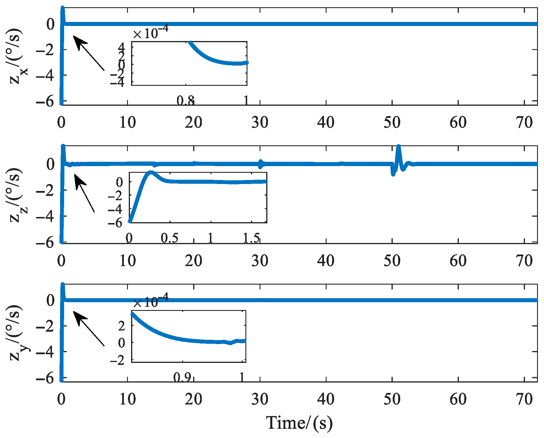
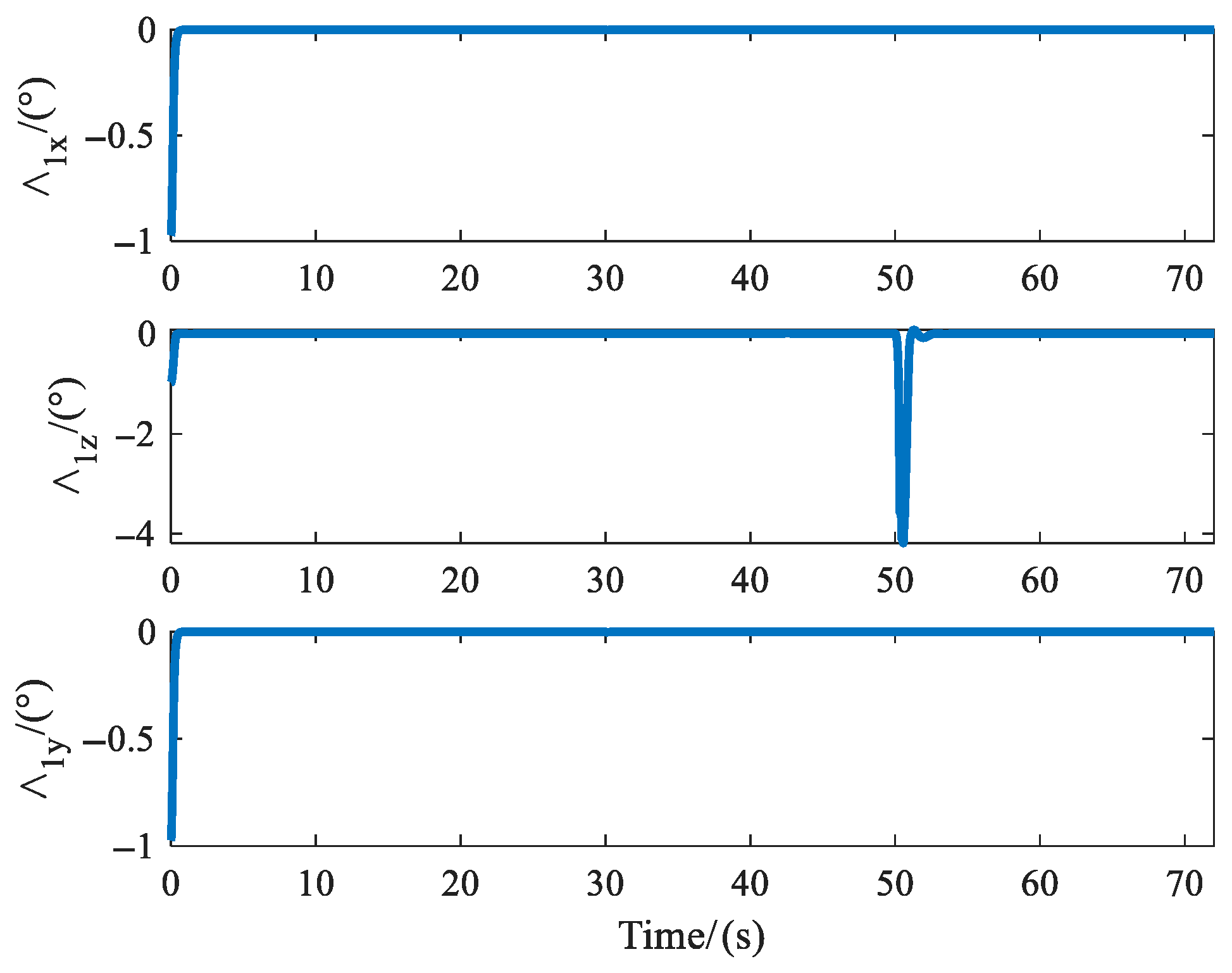
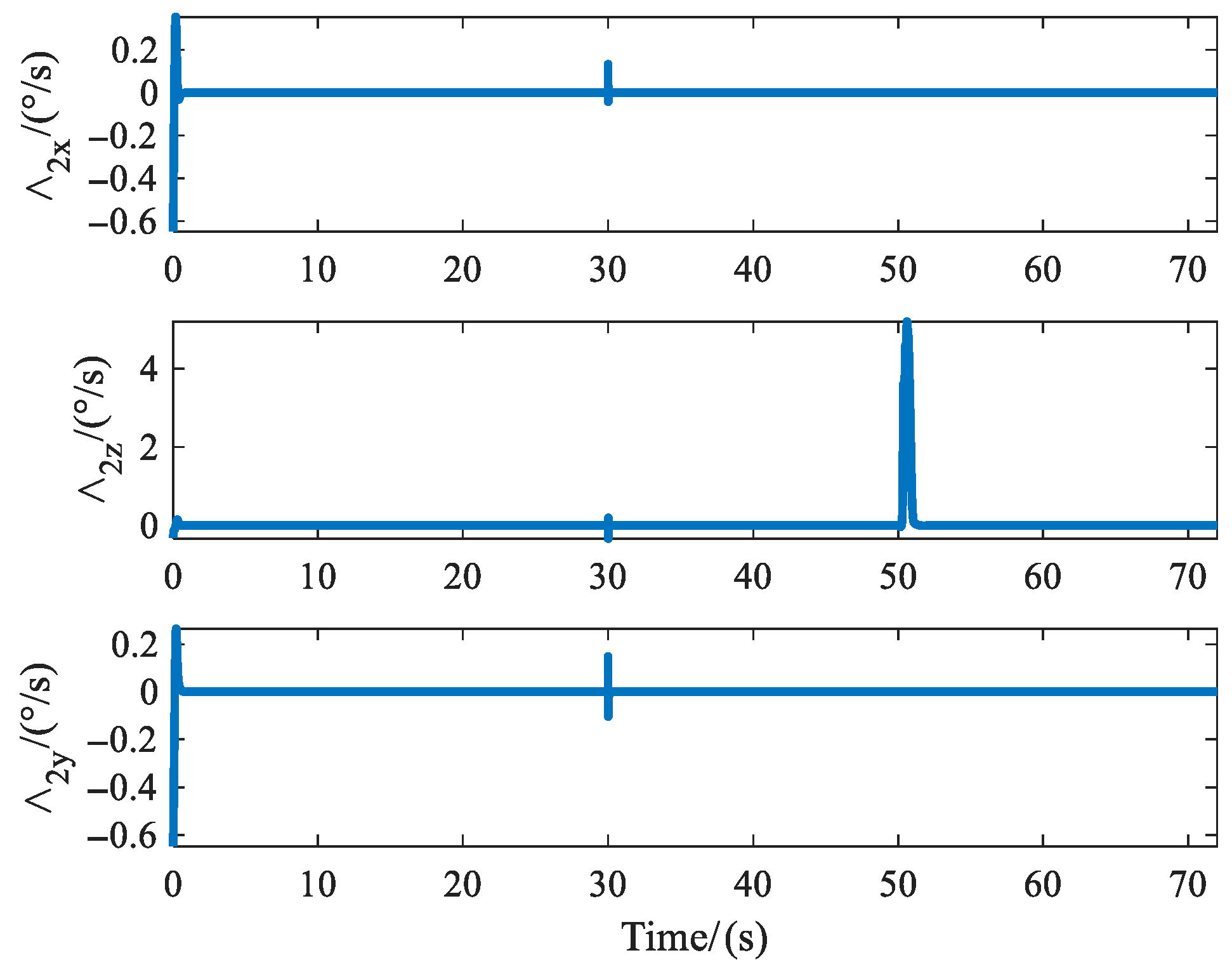
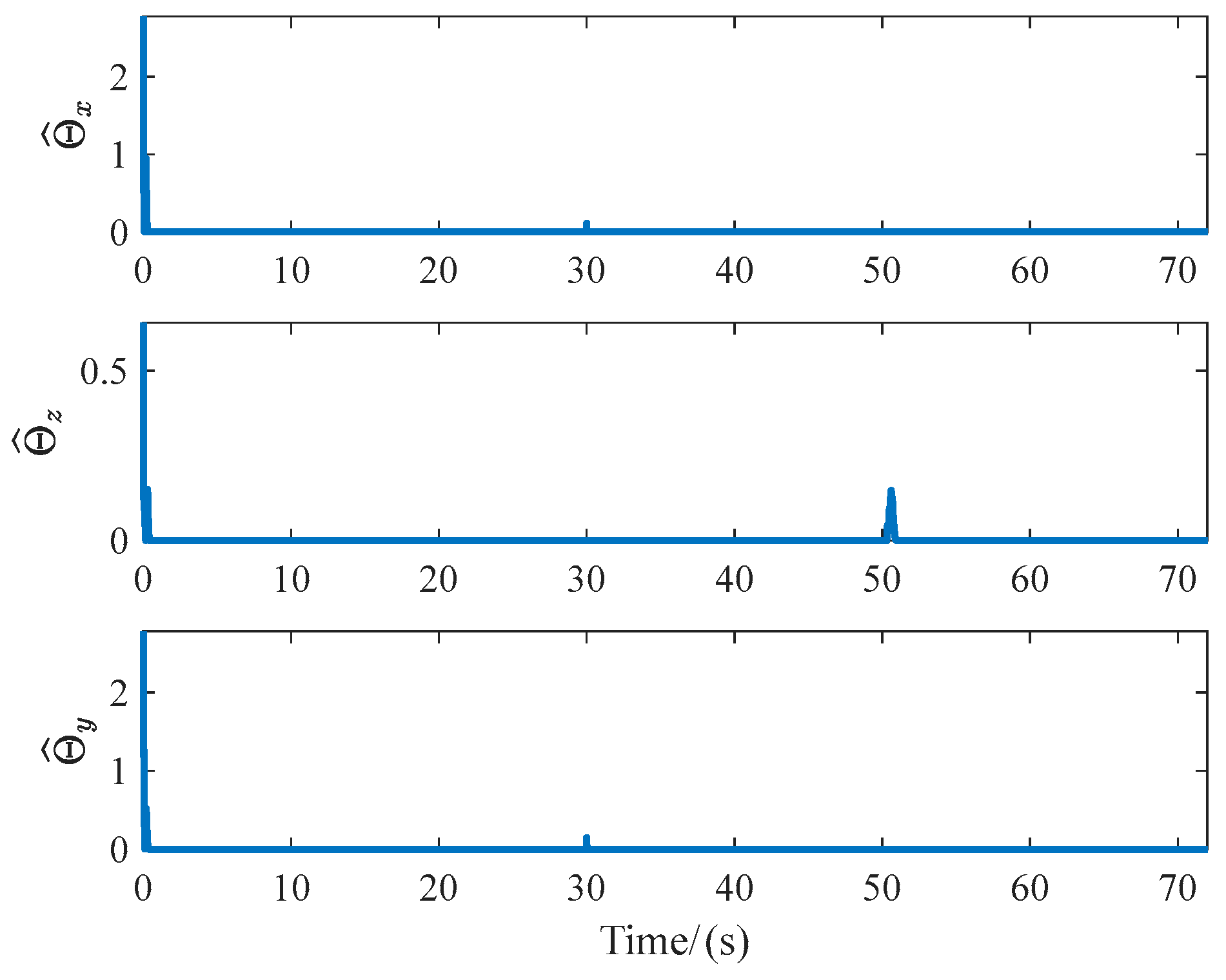
The three-channel attitude angular velocity and attitude angular velocity deviation are displayed in Figure 17 and Figure 18. These figures illustrate that this paper’s controller ensures that the attitude angular velocity is smooth and the attitude angular velocity error is always kept within the constraints throughout the flight. Figure 19, Figure 20, Figure 21 and Figure 22 show the curves of the auxiliary variables Λ 1 , Λ 2 , the filter error z and the network weight estimates Θ ^ , respectively. The designed controllers ensure that they are stable within the appointed time, thus corroborating the conclusions of Theorems 1 and 2.
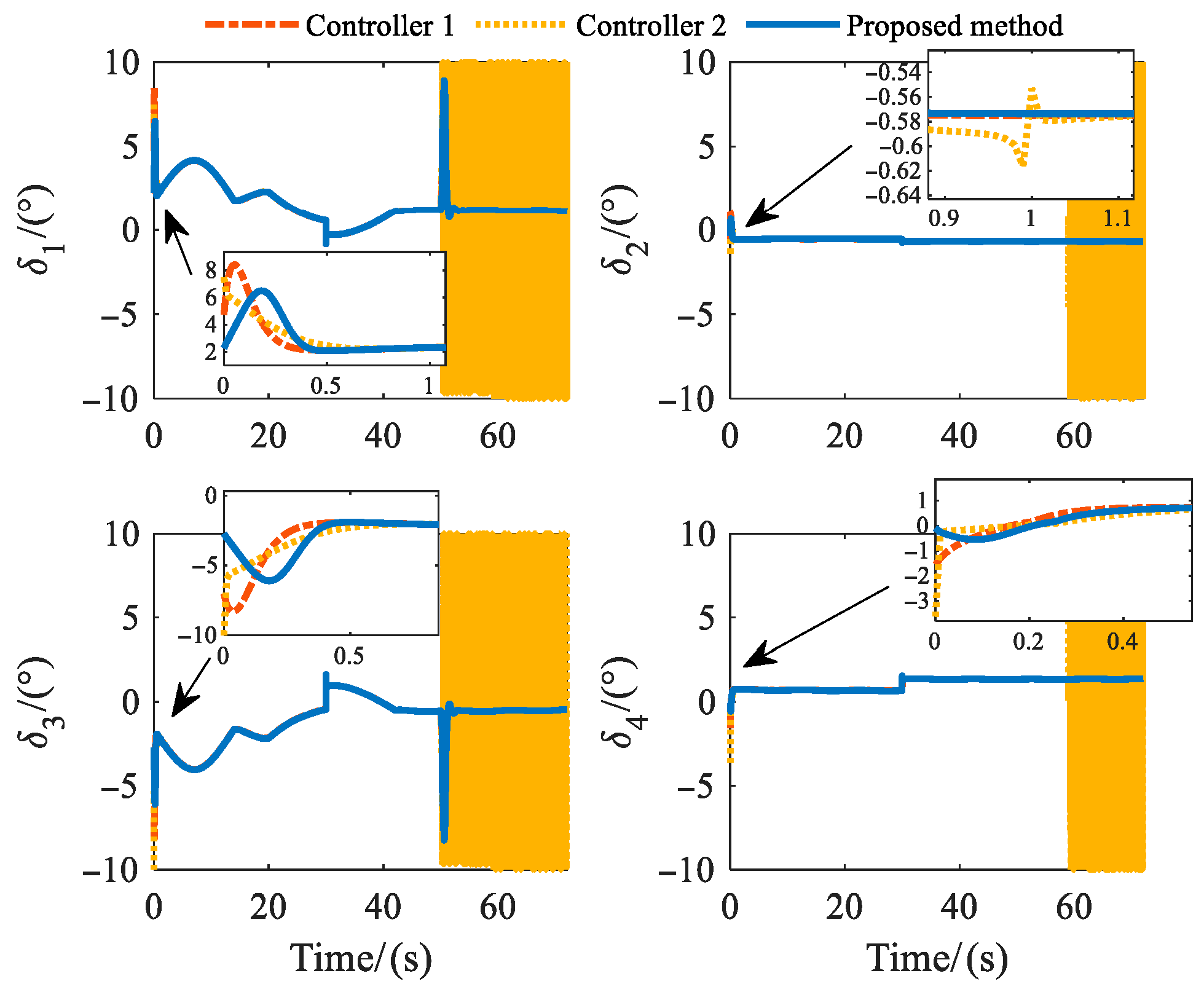
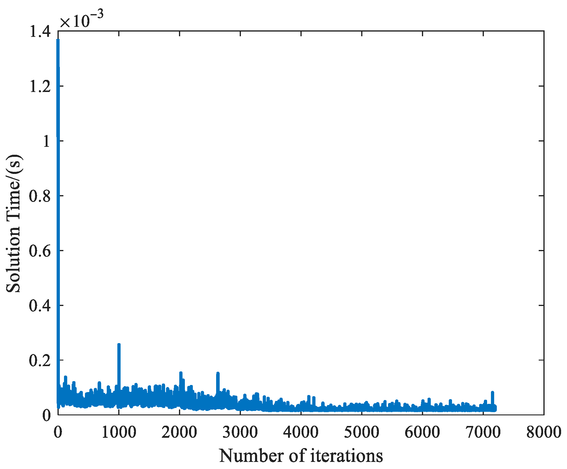
The rudder deflection angle change curve is given in Figure 23, and the time transformation function used in this paper has a smaller rudder deflection angle command at the initial moment because the first and second-order derivatives of the time transformation function in the initial state are both 0, which effectively avoids the actuator saturation problem that can be caused by a large attitude deviation at the initial moment. Moreover, at the convergence moment ( t = 1 ), the time transformation function designed by controller 2 triggers the control command singularity when the simulation step size is small enough because the denominator of the time transformation function in controller 2 is close to 0, but our controller does not have this problem. Figure 24 shows the computation time of the neural network at different simulation steps. It can be seen that the time per computation is less than 0.0015 s, meeting the performance requirements of onboard computers.
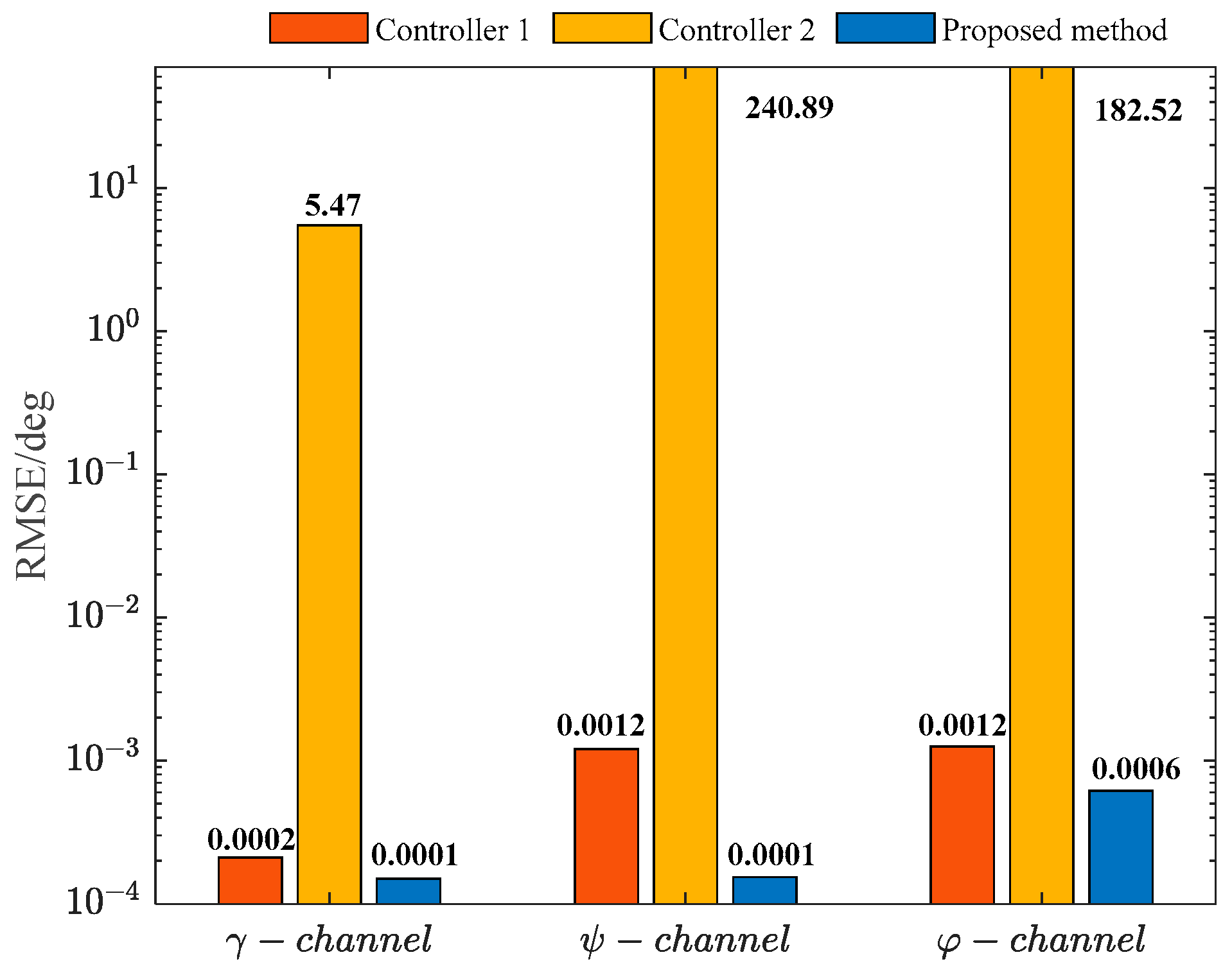
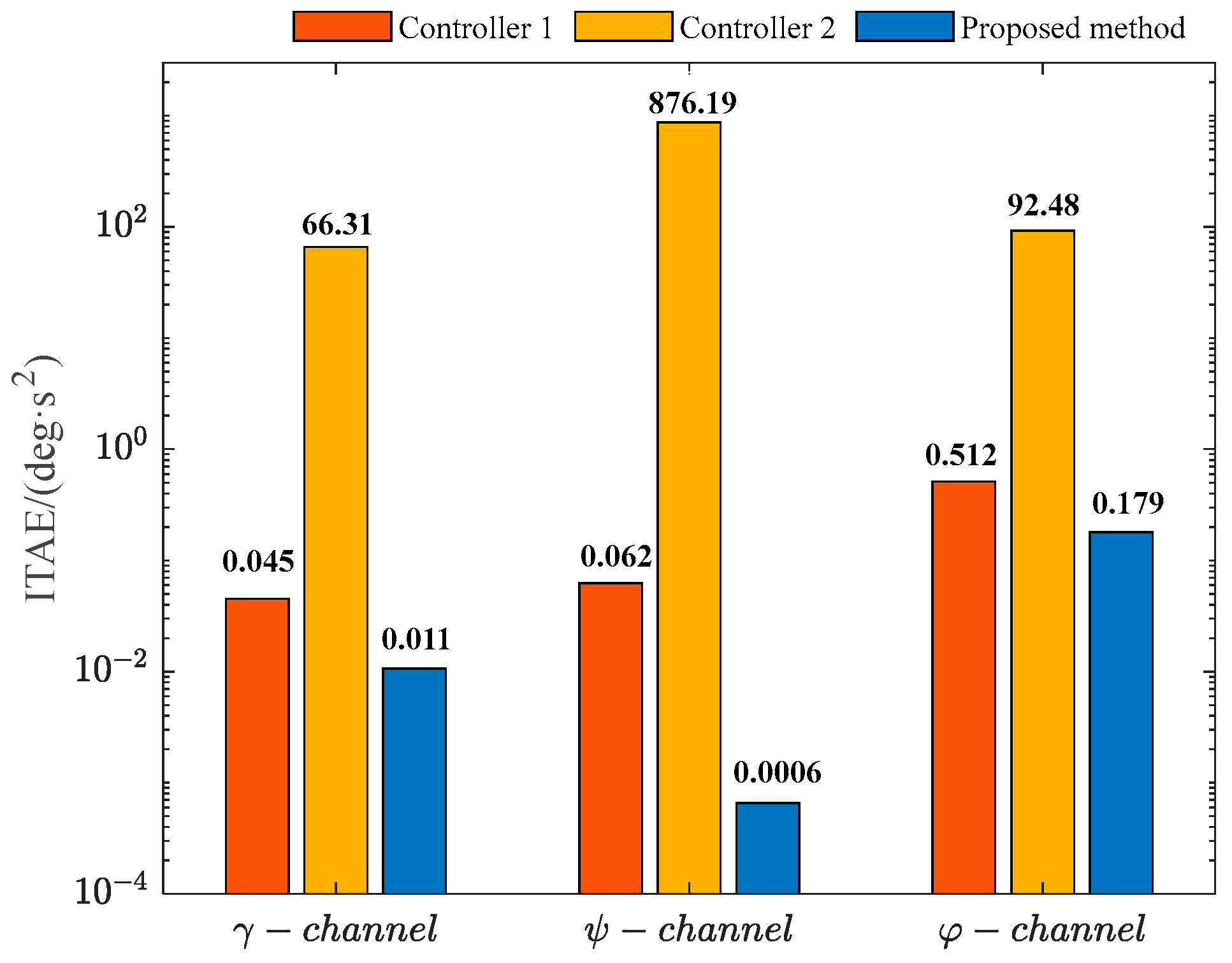
Furthermore, we employ the integral time absolute error (ITAE) and the root mean square error (RMSE) metrics to quantitatively measure capabilities of the controllers discussed earlier.
(1) ITAE = 0 t τ e 1 τ d τ , which represents the size of the error and the convergence speed, with smaller values resulting in better overall controller performance.
(2) RMSE = 1 t 0 t e 1 2 τ d τ , which reflects the average control error, and a smaller value for this metric signifies greater tracking precision by the control method.
The results of the three-channel metrics corresponding to the different controllers are given in Figure 25 and Figure 26.
As shown in Figure 25 and Figure 26, the ITAEs and the RMSEs metric values of this paper’s controller in the γ , ψ and φ channels are significantly lower than those obtained by the other two controllers in different channels. These results indicate that our controller exhibits superior overall performance.
From the above results it is clear that the proposed controller enables the attitude tracking error to converge within the appointed time and remain within the constraints at all times. Moreover, in the face of fast-varying command effects, it can adaptively adjust the performance boundaries according to the flight state, thereby preventing singularity issues that can arise when tracking errors approach or exceed boundaries. Compared to existing prescribed-time and predefined-time controllers, the convergence time of our controller is less conservative, and the first and second-order derivatives of the time conversion function at the initial moment are zero, which reduces the initial control command and effectively reduces the possibility of the actuator saturation problem. Furthermore, the adaptive appointed time filter designed by the method in this paper effectively mitigates the differential explosion problem, and all the signals of the closed-loop system are stabilized at the appointed time. Collectively, these simulation outcomes validate the proposed controller’s capability to address the high-performance attitude tracking challenges for morphing aircraft in the presence of deformation perturbations, sudden aerodynamic uncertainties, asymmetric time-varying constraints, and rapid changes in attitude commands.

5. Conclusions

This paper proposes an appointed-time control method with adaptive boundary adjustment, which effectively solves the high-accuracy stabilization control of morphing aircraft under the influence of time-varying constraints, morphing additional perturbations, abrupt aerodynamic uncertainty disturbances, and fast-varying attitude commands during morphing maneuvers. Compared with the existing morphing aircraft control methods, this method not only achieves a less conservative and precisely regulated system stabilization time but also does not generate the singularity problem at the appointed convergence moment. Moreover, because the initial value of the first and second-order derivatives of the time transition function in the designed appointed-time stable theory is 0, it can make the control quantity generated in the initial large error state smaller, and effectively avoid the problem of actuator saturation. Then, the proposed method is adaptively adjusted based on flight state errors and command changes, which effectively prevents the fragility problem caused by sudden perturbations or fast-changing attitude commands leading to the system error approaching/exceeding the boundaries. Moreover, the UBTF designed herein adeptly handles both asymmetric constraint scenarios and unconstrained control problems within a unified framework. Furthermore, to solve the differential explosion problem, an adaptive appointed-time filter is introduced and the filtering error can be stabilized at a appointed time. Under the action of the designed controller, all the signals in the closed-loop system are guaranteed to be stabilized within the appointed time, and the state error always satisfies the constraints. In summary, the results of simulation and analysis have shown that the proposed controller greatly enhances the control performance.
It is worth noting that this paper assumes that the initial state error of the morphing aircraft remains within the design state constraints. However, for boost-glide morphing aircraft, tracking errors gradually accumulate during the climb phase, making attitude errors at boost-glide separation difficult to predict. Additionally, radial basis functions accurately predict perturbations only when they do not significantly deviate from the training dataset. Therefore, addressing the predefined performance control of deformable aircraft with unknown initial tracking conditions and without reliance on preprocessed datasets will become a key focus for future research. In addition, due to several limitations such as the time and cost, the method is not physically validated in this paper. The above limitations will also be considered and solved in future research.

Author Contributions

Y.Z.: Conceptualization, Methodology, Writing—Review and Editing, Writing—original draft, Visualization, Validation, Investigation, Formal analysis. J.P.: Formal Analysis, Investigation, Data curation, Supervision. Y.G.: Formal Analysis, Investigation, Validation, Visualization, Methodology. N.C.: Conceptualization, Validation, Resources, Supervision. All authors have read and agreed to the published version of the manuscript.

Funding

The authors are grateful to the School of Astronautics, Harbin Institute of Technology. This research was funded by the National Natural Science Foundation of China grant number [62373124] and [62373122].

Data Availability Statement

The datasets presented in this article are not readily available because the data are part of an ongoing study. Requests to access the datasets should be directed to the corresponding author.

Conflicts of Interest

The authors declare that there are no conflicts of interest regarding the publication of this paper.

References

  1. Barbarino, S.; Bilgen, O.; Ajaj, R.M.; Friswell, M.I.; Inman, D.J. A Review of Morphing Aircraft. J. Intell. Mater. Syst. Struct. 2011, 22, 823–877. [Google Scholar] [CrossRef] [Scilit]
  2. Ajaj, R.M.; Beaverstock, C.S.; Friswell, M.I. Morphing Aircraft: The Need for a New Design Philosophy. Aerosp. Sci. Technol. 2016, 49, 154–166. [Google Scholar] [CrossRef] [Scilit]
  3. Bao, C.; Wang, P.; Tang, G. Integrated Method of Guidance, Control and Morphing for Hypersonic Morphing Vehicle in Glide Phase. Chin. J. Aeronaut. 2021, 34, 535–553. [Google Scholar] [CrossRef] [Scilit]
  4. Yue, T.; Zhang, X.; Wang, L.; Ai, J. Flight Dynamic Modeling and Control for a Telescopic Wing Morphing Aircraft via Asymmetric Wing Morphing. Aerosp. Sci. Technol. 2017, 70, 328–338. [Google Scholar] [CrossRef] [Scilit]
  5. Dai, P.; Feng, D.; Zhao, J.; Cui, J.; Wang, C. Asymmetric Integral Barrier Lyapunov Function-Based Dynamic Surface Control of a State-Constrained Morphing Waverider with Anti-Saturation Compensator. Aerosp. Sci. Technol. 2022, 131, 107975. [Google Scholar] [CrossRef] [Scilit]
  6. Chen, M.; Shen, Y.; Skelton, R.E. Model-Based and Markov Data-Based Linearized Tensegrity Dynamics and Analysis of Morphing Airfoils. In Proceedings of the AIAA SCITECH 2024 Forum, Orlando, FL, USA, 8 January 2024; American Institute of Aeronautics and Astronautics: Reston, VA, USA, 2024. [Google Scholar]
  7. Zhao, L.; Jiang, Y.; She, C.-Y.; Balkcom, D.; Dong, H.; Chen, M. Design of A Lightweight Robotic Tensegrity Morphing Airfoil. In Proceedings of the AIAA SCITECH 2026 Forum, Orlando, FL, USA, 12 January 2026; American Institute of Aeronautics and Astronautics: Reston, VA, USA, 2026. [Google Scholar]
  8. Shen, Y.; Chen, M.; Skelton, R.E. Markov Data-Based Reference Tracking Control to Tensegrity Morphing Airfoils. Eng. Struct. 2023, 291, 116430. [Google Scholar] [CrossRef] [Scilit]
  9. Parancheerivilakkathil, M.S.; Pilakkadan, J.S.; Ajaj, R.M.; Amoozgar, M.; Asadi, D.; Zweiri, Y.; Friswell, M.I. A Review of Control Strategies Used for Morphing Aircraft Applications. Chin. J. Aeronaut. 2024, 37, 436–463. [Google Scholar] [CrossRef] [Scilit]
  10. Yan, B.; Li, Y.; Dai, P.; Liu, S. Aerodynamic Analysis, Dynamic Modeling, and Control of a Morphing Aircraft. J. Aerosp. Eng. 2019, 32, 04019058. [Google Scholar] [CrossRef] [Scilit]
  11. Cai, G.; Yang, Q.; Mu, C.; Li, X. Design of Linear Parameter-Varying Controller for Morphing Aircraft Using Inexact Scheduling Parameters. IET Control Theory Appl. 2023, 17, 493–503. [Google Scholar] [CrossRef] [Scilit]
  12. Lee, J.; Kim, S.; Jung, S.; Lee, H.; Kim, Y. Linear Parameter-Varying Control of Variable Span-Sweep Morphing Aircraft. In Proceedings of the AIAA Scitech 2019 Forum, San Diego, CA, USA, 7 January 2019; American Institute of Aeronautics and Astronautics: Reston, VA, USA, 2019. [Google Scholar]
  13. Jie, Z. H∞ Robust Adaptive Controller for a Morphing Aircraft Based on SRAD and LPV Model. In Proceedings of the 2018 Chinese Control And Decision Conference (CCDC), Shenyang, China, 9–11 June 2018; pp. 5250–5255. [Google Scholar]
  14. Liu, J.; Shan, J.; Wang, J.; Rong, J. Incremental Sliding-Mode Control and Allocation for Morphing-Wing Aircraft Fast Manoeuvring. Aerosp. Sci. Technol. 2022, 131, 107959. [Google Scholar] [CrossRef] [Scilit]
  15. Zhang, H.; Wang, P.; Tang, G.; Bao, W. Fuzzy Disturbance Observer-Based Dynamic Sliding Mode Control for Hypersonic Morphing Vehicles. Aerosp. Sci. Technol. 2023, 142, 108633. [Google Scholar] [CrossRef] [Scilit]
  16. Dai, P.; Yan, B.; Han, T.; Liu, S. Barrier Lyapunov Function Based Model Predictive Control of a Morphing Waverider with Input Saturation and Full-State Constraints. IEEE Trans. Aerosp. Electron. Syst. 2023, 59, 3071–3081. [Google Scholar] [CrossRef] [Scilit]
  17. Guo, T.; Hou, Z.; Zhu, B. Dynamic Modeling and Active Morphing Trajectory-Attitude Separation Control Approach for Gull-Wing Aircraft. IEEE Access 2017, 5, 17006–17019. [Google Scholar] [CrossRef] [Scilit]
  18. Wu, K.; Zhang, P.; Wu, H. A New Control Design for a Morphing UAV Based on Disturbance Observer and Command Filtered Backstepping Techniques. Sci. China Technol. Sci. 2019, 62, 1845–1853. [Google Scholar] [CrossRef] [Scilit]
  19. Gong, L.; Wang, Q.; Dong, C. Disturbance Rejection Control of Morphing Aircraft Based on Switched Nonlinear Systems. Nonlinear Dyn. 2019, 96, 975–995. [Google Scholar] [CrossRef] [Scilit]
  20. Chu, L.; Li, Q.; Gu, F.; Du, X.; He, Y.; Deng, Y. Design, Modeling, and Control of Morphing Aircraft: A Review. Chin. J. Aeronaut. 2022, 35, 220–246. [Google Scholar] [CrossRef] [Scilit]
  21. Zhang, H.; Wang, P.; Tang, G.; Bao, W. Fixed-Time Attitude Control for Hypersonic Morphing Vehicles: A Dynamic Memory Event-Triggering Approach. Aerosp. Sci. Technol. 2024, 155, 109577. [Google Scholar] [CrossRef] [Scilit]
  22. Zhang, H.; Wang, P.; He, R.; Tang, G.; Bao, W. Event-Triggered Attitude Control for Hypersonic Morphing Vehicles Using Fixed-Time Control Technique. Aerosp. Sci. Technol. 2024, 144, 108773. [Google Scholar] [CrossRef] [Scilit]
  23. Chen, H.; Wang, P.; Tang, G. Fuzzy Disturbance Observer-Based Fixed-Time Sliding Mode Control for Hypersonic Morphing Vehicles with Uncertainties. IEEE Trans. Aerosp. Electron. Syst. 2023, 59, 3521–3530. [Google Scholar] [CrossRef] [Scilit]
  24. Liang, X.; Wang, Q.; Xu, B.; Dong, C. Back-Stepping Fault-Tolerant Control for Morphing Aircraft Based on Fixed-Time Observer. Int. J. Control Autom. Syst. 2021, 19, 3924–3936. [Google Scholar] [CrossRef] [Scilit]
  25. Tang, H.; Chen, Y. Composite Observer-Based Resilient MPC for Heterogeneous UAV-UGV Systems Under Hybrid Cyberattacks. IEEE Trans. Aerosp. Electron. Syst. 2025, 61, 8277–8290. [Google Scholar] [CrossRef] [Scilit]
  26. Jiang, J.; Tang, J.; Liu, M.; Li, Y.; Chen, H.; Cao, D. A Data-Driven Neural Model Predictive Controller for Multi-Layer Nonlinear Vibration Isolation System. Aerosp. Sci. Technol. 2025, 166, 110583. [Google Scholar] [CrossRef] [Scilit]
  27. Ju, X.; Wei, C.; Xu, H.; Wang, F. Fractional-Order Sliding Mode Control with a Predefined-Time Observer for VTVL Reusable Launch Vehicles under Actuator Faults and Saturation Constraints. ISA Trans. 2022, 129, 55–72. [Google Scholar] [CrossRef] [Scilit]
  28. Xiao, Y. Predefined-Time Robust Attitude Tracking Control of Flexible Spacecraft with Continuous and Nonsingular Performance. Aerosp. Sci. Technol. 2025, 159, 110000. [Google Scholar] [CrossRef] [Scilit]
  29. Dong, T. Terminal Sliding Mode Attitude Tracking Control for Unmanned Vehicle with Predefined-Time Stability. Aerosp. Sci. Technol. 2023, 142, 108669. [Google Scholar] [CrossRef] [Scilit]
  30. Xu, S.; Wei, C.; Zhang, L.; Mu, R. Neural Network Based Adaptive Nonsingular Practical Predefined-Time Fault-Tolerant Control for Hypersonic Morphing Aircraft. Chin. J. Aeronaut. 2023, 37, 421–435. [Google Scholar] [CrossRef] [Scilit]
  31. Lu, X.; Wang, J.; Wang, Y.; Chen, J. Neural Network Observer-Based Predefined-Time Attitude Control for Morphing Hypersonic Vehicles. Aerosp. Sci. Technol. 2024, 152, 109333. [Google Scholar] [CrossRef] [Scilit]
  32. Lv, J.; Ju, X.; Wang, C. Neural Network-Based Nonconservative Predefined-Time Backstepping Control for Uncertain Strict-Feedback Nonlinear Systems. IEEE Trans. Neural Netw. Learn. Syst. 2023, 35, 16562–16573. [Google Scholar] [CrossRef] [Scilit]
  33. Zhao, K.; Xie, Y.; Xu, S.; Zhang, L. Adaptive Neural Appointed-Time Prescribed Performance Control for the Manipulator System via Barrier Lyapunov Function. J. Frankl. Inst. 2024, 362, 107468. [Google Scholar] [CrossRef] [Scilit]
  34. Pal, A.K.; Kamal, S.; Nagar, S.K.; Bandyopadhyay, B.; Fridman, L. Design of Controllers with Arbitrary Convergence Time. Automatica 2020, 112, 108710. [Google Scholar] [CrossRef] [Scilit]
  35. Pal, A.K.; Kamal, S.; Yu, X.; Nagar, S.K.; Bandyopadhyay, B. Free-Will Arbitrary Time Terminal Sliding Mode Control. IEEE Trans. Circuits Syst. II Express Briefs 2022, 69, 3189–3193. [Google Scholar] [CrossRef] [Scilit]
  36. Li, D.; Zhang, L.; Xu, S.; Li, Y.; Cui, N. Appointed Time Control for Flexible Satellite with Active Vibration Suppression. Adv. Space Res. 2024, 74, 3284–3296. [Google Scholar] [CrossRef] [Scilit]
  37. Zhang, L.; Liu, J.; Cui, N. Backstepping Control for a Two-Link Manipulator with Appointed-Time Convergence. ISA Trans. 2022, 128, 208–219. [Google Scholar] [CrossRef] [Scilit]
  38. Wang, N.; Gao, Y.; Zhang, X. Data-Driven Performance-Prescribed Reinforcement Learning Control of an Unmanned Surface Vehicle. IEEE Trans. Neural Netw. Learn. Syst. 2021, 32, 5456–5467. [Google Scholar] [CrossRef] [Scilit]
  39. Bechlioulis, C.P.; Rovithakis, G.A. Robust Adaptive Control of Feedback Linearizable MIMO Nonlinear Systems with Prescribed Performance. IEEE Trans. Autom. Control 2008, 53, 2090–2099. [Google Scholar] [CrossRef] [Scilit]
  40. Xu, S.; Guan, Y.; Wei, C.; Li, Y.; Xu, L. Reinforcement-Learning-Based Tracking Control with Fixed-Time Prescribed Performance for Reusable Launch Vehicle under Input Constraints. Appl. Sci. 2022, 12, 7436. [Google Scholar] [CrossRef] [Scilit]
  41. Shao, X.; Hu, Q.; Shi, Y.; Jiang, B. Fault-Tolerant Prescribed Performance Attitude Tracking Control for Spacecraft Under Input Saturation. IEEE Trans. Control Syst. Technol. 2020, 28, 574–582. [Google Scholar] [CrossRef] [Scilit]
  42. Gong, L.; Wang, Q.; Dong, C.; Zhong, K. Prescribed Performance Control of Morphing Aircraft Based on Switched Nonlinear Systems and Reinforcement Learning. Meas. Control 2019, 52, 608–624. [Google Scholar] [CrossRef] [Scilit]
  43. Meng, F.; Wang, T.; Chen, G. Prescribed Performance-Based Active Anti-Disturbance Backstepping Control for Morphing Aircraft. Aerosp. Sci. Technol. 2024, 152, 109386. [Google Scholar] [CrossRef] [Scilit]
  44. Bu, X.; Hua, C.; Lv, M.; Wu, Z. Flight Control of Waverider Vehicles with Fragility-Avoidance Prescribed Performance. IEEE Trans. Aerosp. Electron. Syst. 2023, 59, 5248–5261. [Google Scholar] [CrossRef] [Scilit]
  45. Ji, R.; Li, D.; Ma, J.; Ge, S.S. Saturation-Tolerant Prescribed Control of MIMO Systems with Unknown Control Directions. IEEE Trans. Fuzzy Syst. 2022, 30, 5116–5127. [Google Scholar] [CrossRef] [Scilit]
  46. Zheng, D.-D.; Li, X.; Ren, X.; Na, J. Intelligent Control for Robotic Manipulator with Adaptive Learning Rate and Variable Prescribed Performance Boundaries. J. Frankl. Inst. 2023, 360, 7037–7062. [Google Scholar] [CrossRef] [Scilit]
  47. Bu, X. Saturated Control with Variable Prescribed Performance Applied to the Manipulator of UAV. IEEE J. Miniat. Air Space Syst. 2023, 4, 212–220. [Google Scholar] [CrossRef] [Scilit]
  48. Bu, X.; Jiang, B.; Feng, Y. Non-Fragile Tracking Control of Constrained Waverider Vehicles with Readjusting Prescribed Performance. Nonlinear Dyn. 2022, 108, 3657–3669. [Google Scholar] [CrossRef] [Scilit]
  49. Bu, X.; Jiang, B.; Lei, H. Nonfragile Quantitative Prescribed Performance Control of Waverider Vehicles with Actuator Saturation. IEEE Trans. Aerosp. Electron. Syst. 2022, 58, 3538–3548. [Google Scholar] [CrossRef] [Scilit]
  50. Bu, X.; Lv, M.; Lei, H.; Cao, J. Fuzzy Neural Pseudo Control with Prescribed Performance for Waverider Vehicles: A Fragility-Avoidance Approach. IEEE Trans. Cybern. 2023, 53, 4986–4999. [Google Scholar] [CrossRef] [Scilit]
  51. Zhao, K.; Song, Y.; Chen, C.L.P.; Chen, L. Control of Nonlinear Systems under Dynamic Constraints: A Unified Barrier Function-Based Approach. Automatica 2020, 119, 109102. [Google Scholar] [CrossRef] [Scilit]
  52. Jin, X. Adaptive Fixed-Time Control for MIMO Nonlinear Systems with Asymmetric Output Constraints Using Universal Barrier Functions. IEEE Trans. Autom. Control 2019, 64, 3046–3053. [Google Scholar] [CrossRef] [Scilit]
  53. Dai, P.; Yan, B.; Liu, R.; Liu, S.; Wang, M. Modeling and Nonlinear Model Predictive Control of a Variable-Sweep-Wing Morphing Waverider. IEEE Access 2021, 9, 63510–63520. [Google Scholar] [CrossRef] [Scilit]
  54. Yang, G.T.; Tang, S.J.; Zhao, L.D.; Guo, J. Dynamic Modeling and Response of a Morphing UAV with Variable Sweep and Variable Span. Acta Armamentarii 2014, 35, 102. [Google Scholar] [CrossRef]
  55. Pu, J.; Zhang, Y.; Guan, Y.; Cui, N. Recurrent Neural Network-Based Predefined Time Control for Morphing Aircraft with Asymmetric Time-Varying Constraints. Appl. Math. Model. 2024, 135, 578–600. [Google Scholar] [CrossRef] [Scilit]
  56. Chen, H.; Wang, P.; Tang, G. Prescribed-Time Control for Hypersonic Morphing Vehicles with State Error Constraints and Uncertainties. Aerosp. Sci. Technol. 2023, 142, 108671. [Google Scholar] [CrossRef] [Scilit]
  57. Jia, F.; Wang, X.; Zhou, X. Robust Adaptive Prescribed Performance Control for a Class of Nonlinear Pure-Feedback Systems. Int. J. Robust Nonlinear Control 2019, 29, 3971–3987. [Google Scholar] [CrossRef] [Scilit]
  58. Ni, J.; Ahn, C.K.; Liu, L.; Liu, C. Prescribed Performance Fixed-Time Recurrent Neural Network Control for Uncertain Nonlinear Systems. Neurocomputing 2019, 363, 351–365. [Google Scholar] [CrossRef] [Scilit]
  59. Polyakov, A. Nonlinear Feedback Design for Fixed-Time Stabilization of Linear Control Systems. IEEE Trans. Autom. Control 2012, 57, 2106–2110. [Google Scholar] [CrossRef] [Scilit]
  60. Sánchez-Torres, J.D.; Gómez-Gutiérrez, D.; López, E.; Loukianov, A.G. A Class of Predefined-Time Stable Dynamical Systems. IMA J. Math. Control Inf. 2018, 35, i1–i29. [Google Scholar] [CrossRef] [Scilit]
  61. Wu, C.; Yan, J.; Shen, J.; Wu, X.; Xiao, B. Predefined-Time Attitude Stabilization of Receiver Aircraft in Aerial Refueling. IEEE Trans. Circuits Syst. II 2021, 68, 3321–3325. [Google Scholar] [CrossRef] [Scilit]
  62. Wang, F.; Gao, Z.; Xie, X.; Zhou, C.; Hua, C. Adaptive Prescribed-Time Filtered Control Design for a Full-State Constrained Nonlinear System. IEEE Trans. Cybern. 2025, 55, 321–331. [Google Scholar] [CrossRef] [Scilit]
  63. Li, J.; Zhang, J.; Ye, J.; Shao, L.; Bu, X. Optimal Midcourse Guidance with Terminal Relaxation and Range Convex Optimization. Aerospace 2025, 12, 618. [Google Scholar] [CrossRef] [Scilit]
  64. Quartullo, R.; Bianchini, G.; Garulli, A.; Giannitrapani, A. Robust Variable-Horizon MPC with Adaptive Terminal Constraints. Automatica 2025, 179, 112465. [Google Scholar] [CrossRef] [Scilit]
  65. Zhang, T.; Xia, M.; Yi, Y. Adaptive Neural Dynamic Surface Control of Strict-Feedback Nonlinear Systems with Full State Constraints and Unmodeled Dynamics. Automatica 2017, 81, 232–239. [Google Scholar] [CrossRef] [Scilit]
Figure 1. Shape of the aircraft.
Aerospace 13 00441 g001
Figure 2. Rudder distribution of the aircraft.
Aerospace 13 00441 g002
Figure 3. Time history of κ ( t ) .
Aerospace 13 00441 g003
Figure 4. Time history of κ ˙ ( t ) .
Aerospace 13 00441 g004
Figure 5. Time history of κ ¨ ( t ) .
Aerospace 13 00441 g005
Figure 6. The structure of this paper’s controller.
Aerospace 13 00441 g006
Figure 7. Simulation results with T c = 0.4 .
Aerospace 13 00441 g007
Figure 8. Simulation results with T c = 0.8 .
Aerospace 13 00441 g008
Figure 9. Simulation results with T c = 1.2 .
Aerospace 13 00441 g009
Figure 10. Flight envelope of the morphing aircraft.
Aerospace 13 00441 g010
Figure 11. Time histories of the roll angle.
Aerospace 13 00441 g011
Figure 12. Time histories of the roll angle error.
Aerospace 13 00441 g012
Figure 13. Time histories of the pitch angle.
Aerospace 13 00441 g013
Figure 14. Time histories of the pitch angle error.
Aerospace 13 00441 g014
Figure 15. Time histories of the yaw angle.
Aerospace 13 00441 g015
Figure 16. Time histories of the yaw angle error.
Aerospace 13 00441 g016
Figure 17. Time histories of angular rate.
Aerospace 13 00441 g017
Figure 18. Time histories of angular rate error.
Aerospace 13 00441 g018
Figure 19. Time histories of Λ 1 .
Aerospace 13 00441 g019
Figure 20. Time histories of Λ 2 .
Aerospace 13 00441 g020
Figure 21. Time histories of z .
Aerospace 13 00441 g021
Figure 22. Time histories of Θ ^ .
Aerospace 13 00441 g022
Figure 23. Time histories of the rudder declination angles.
Aerospace 13 00441 g023
Figure 24. Neural network computation time.
Aerospace 13 00441 g024
Figure 25. ITAE indices of different controllers.
Aerospace 13 00441 g025
Figure 26. RMSE indices of different controllers.
Aerospace 13 00441 g026
Table 1. Settings of the initial values.
CaseCase 1Case 2Case 3Case 4Case 5Case 6
Initial   value   of   x 1 φ −1 deg−2 deg−3 deg−4 deg1 deg2 deg
Table 2. The constraint function and controller parameters.
ControllerController Parameters
Proposed controller α 1 = α 2 = α 4 = 1 , α 3 = 5 , α 5 = 10 λ 1 = 0.01 , λ 2 = λ 3 = 0.1 m 1 = 50 , m 2 = 10 , m 3 = 100 ϖ = 0.01 b _ 1 j = 8 e 2 t + 0.3 + ρ a ( t ) b ¯ 1 j = 4 e t + 0.2 + ρ a ( t ) b _ 2 j = 15 e 2 t + 10 + ρ a ( t ) b ¯ 2 j = 15 e 2 t + 15 + ρ a ( t )
Table 3. Structural parameters of the morphing aircraft.
ParametersValue
Mass   of   the   fuselage   m 0 850 kg
Cross-section area Sref2.2 m2
Reference length L1.6 m
Mass   of   the   morphing   wings   m 1 , m 2 52 kg
Table 4. Parameter selection for different controllers.
ControllerController Parameters
Proposed controller α 1 = α 2 = α 4 = 0.5 , α 3 = 6 , α 5 = 40 λ 1 = 0.01 , λ 2 = 1 , λ 3 = 0.1 m 1 = 20 , m 2 = 1 , m 3 = 100 T c = 0.001 , ϖ = 0.001 k ρ 1 = 10 , k ρ 2 = 2 b _ 1 j = 8 e 2 t + 0.3 + ρ a ( t ) b ¯ 1 j = 4 e t + 0.2 + ρ a ( t ) b _ 2 j = 15 e 2 t + 10 + ρ a ( t ) b ¯ 2 j = 15 e 2 t + 15 + ρ a ( t )
Controller 1 α = 0.1 , T c = 1 , χ s = 15 , ε = 0.01
Controller 2 r 0 = 1.2 , T p = 1 , κ a = 2 , κ b = 3 c 1 = c 2 = c 3 = c 4 = 1 k a = 8 e 2 t + 0.3 , k b = 15 e 2 t + 15
Disclaimer/Publisher’s Note: The statements, opinions and data contained in all publications are solely those of the individual author(s) and contributor(s) and not of MDPI and/or the editor(s). MDPI and/or the editor(s) disclaim responsibility for any injury to people or property resulting from any ideas, methods, instructions or products referred to in the content.