Article

Fast Data-Driven Noise Prediction for an Aircraft in Unconventional Configuration Using Flight Test Data

by
Dominik Eisenhut
* and
Andreas Strohmayer
University of Stuttgart, Institute of Aircraft Design, 70569 Stuttgart, Germany
*
Author to whom correspondence should be addressed.
Aerospace 2026, 13(3), 292; https://doi.org/10.3390/aerospace13030292
Submission received: 27 February 2026 / Revised: 17 March 2026 / Accepted: 17 March 2026 / Published: 19 March 2026

Abstract

New, highly integrated, disruptive aircraft concepts are being devised to reduce aviation’s environmental footprint, but their performance is oftentimes challenging for the aircraft designer to assess. Furthermore, these novel aircraft often introduce new risks, such as noise, that cannot be addressed quickly by available methods. Overall, in the pursuit of more environmental friendly aircraft configurations and the lack of methods to design such aircraft, aircraft-level trade-offs between noise and performance are challenging. The present study aims to close this gap by using a machine learning-based approach for one unconventional aircraft to investigate usability in the early stages of aircraft design. Based on overflight noise measurements, noise models for this aircraft are created with different approaches and base models. The single-output models show good performance, with mean absolute errors around 1 dB, good rank correlations and R2 scores above 0.9. Support vector regression provides reasonably good agreement from experiments requiring only a small effort to set up; Neural Networks achieve better performance, but increased effort is required to obtain the model.

1. Introduction

Aviation, like many other industries, contributes to climate change through emissions. Different initiatives such as Flightpath 2050 [1] and Fly the Green Deal [2] aim at limiting this impact and making aviation a climate-neutral industry by 2050. One solution may be the use of novel aircraft concepts that closely integrate components to promote positive synergies; an example of this approach is Distributed Electric Propulsion (DEP), used by aircraft such as the Electra.aero EL2 [3] and EL9 [4]. However, at the aircraft level, methods are often lacking to assess the performance benefit that these innovations aim to provide. Furthermore, this close integration can cause unwanted effects such as noise [5,6,7]. Apart from annoyance, this also poses a certification risk, when, for example, ICAO Annex 16 [8] limits cannot be achieved. Here, methodologies are also lacking to make design trade-offs at the aircraft level [9,10,11]. Our novel approach in this study is to use machine learning (ML) to bridge the gap between aircraft-level assessment and high(er)-fidelity simulations.
The interest in applications of ML to aviation is rapidly growing, as highlighted by many review papers [11,12,13,14,15,16]. Several previous works have taken a similar direction to the present study. For example, with a focus on aeroacoustics in propeller aircraft, Poggi et al. [17] investigated a single isolated propeller based on high-fidelity data, and they also examined six counter-rotating propellers as a DEP configuration [18]. Both studies aim more at optimization on the propeller level than finding an optimum aircraft configuration. Similarly, Thurman and Zawodny [19] used a lower-fidelity database for hovering rotors for similar purposes. All three of these studies leave a gap in aircraft-level assessment, as aircraft-level metrics and trade-offs are missing. Furthermore, integration aspects are not covered in studies that assess isolated components. Apart from these studies, Manghnani et al. [20,21,22] focus on developing an ML model for aircraft design to be utilized for general aviation and advanced air mobility. The general approach is different, applying lower-fidelity methods (panel method) as well as a generic geometry that covers only the wing and propeller instead of the full aircraft [20,21,22].
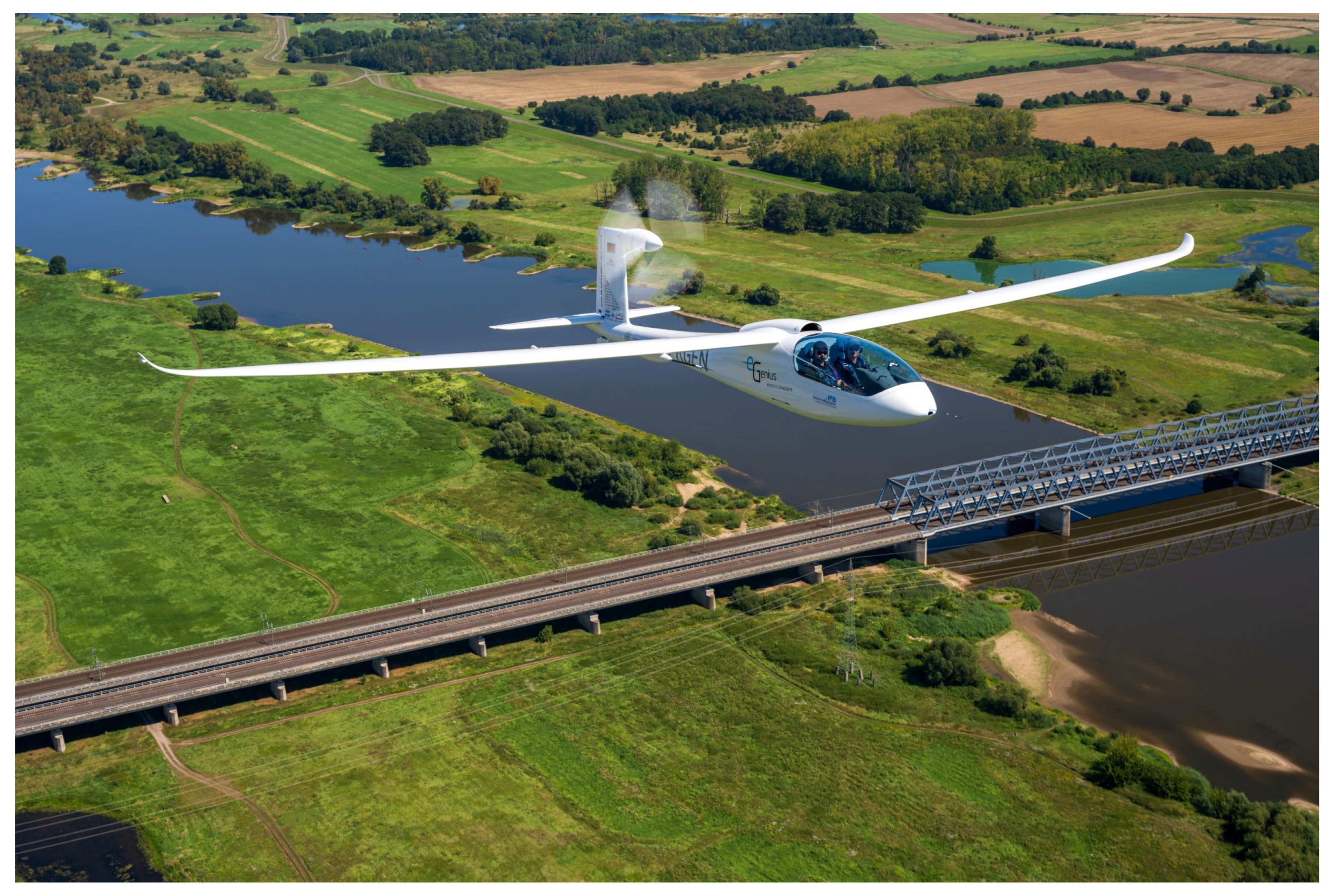
The present paper covers this topic by looking at the University of Stuttgart Institute of Aircraft Design’s aircraft, e-Genius [23]. Figure 1 shows the two-seat electric aircraft with its propeller mounted in front of the vertical tail. Due to this unconventional design and the all-electric power train, unique features are apparent. An extensive noise measurement campaign was conducted in August 2025.
The use of an ML-based surrogate is a flexible approach that can be applied to various aircraft configurations. The research question addressed in this paper is whether an ML model can be used to predict noise with adequate accuracy at the preliminary aircraft design stage. In the present work, this methodology is applied to the e-Genius configuration. In the future, an enhanced model will be trained based on higher-fidelity simulation data; the necessary database for this is currently being created. This future step will address propeller performance in addition to noise, thereby bridging the gap and allowing an aircraft-level trade-off.
The remainder of the paper is structured as follows. First, the materials and methods are explained. This methodology includes a description of the noise measurement campaign and the resulting data set. Second, we describe the ML approach, including all the methods used. Third, we summarize the results of the different trained surrogates, including single- and multi-output models. Fourth, we discuss the accuracy and create two additional models addressing the findings from the initial models. Finally, we present our conclusion and an outlook on future research.

2. Materials and Methods

First, the Materials and Methods Section covers the underlying experimental noise database used for the training and validation of the surrogates. Second, we introduce the investigated models and their tuned hyperparameters as well as the general approach.

2.1. Experimental Noise Database

The lessons learned from the e-Genius noise test campaign in 2024 [24] have been applied to this year’s campaign with the following changes. The e-Genius has been equipped with a Global Positioning System–Real-Time Kinematics (GPS-RTK) receiver, which allows an accuracy of approximately 1 cm in all three dimensions. This is enabled by using the SAPOS service as a ground reference station. Hence, the exact position of the aircraft in relation to the microphones can be tracked, making it possible to correct measurements and calculate additional metrics.
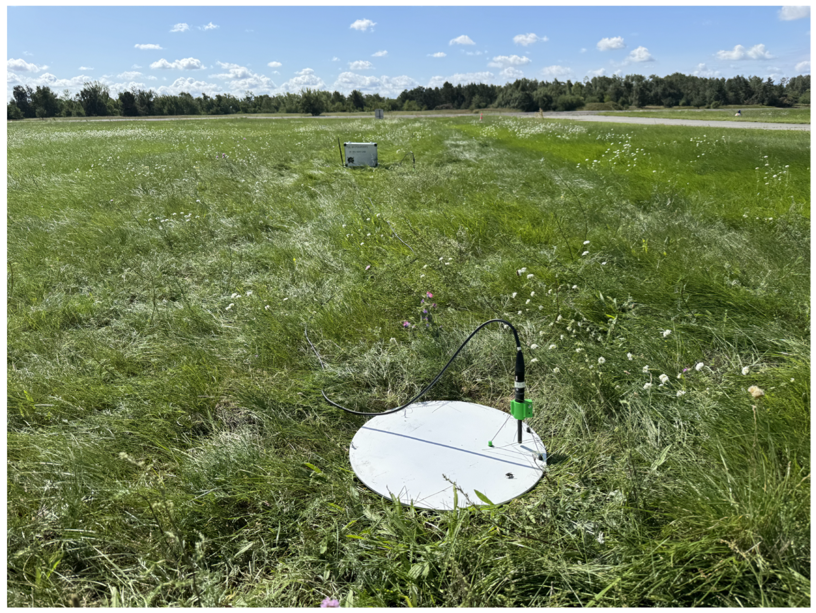
The measurement setup consists of twelve microphones, divided across four measurement boxes—two boxes with two channels each and two boxes with four channels each. The microphones are mounted 5 mm above a ground plate facing downward according to the ICAO Annex 16 Volume I [8] (compare Figure 2). Furthermore, each microphone is calibrated to a 1000 Hz tone at 94 dB. Time synchronization is achieved by a beeping device, encoding time information, at least once per measurement box and recording. Due to the sampling rate of the recordings, 44.1 kHz, the theoretical maximum frequency that can be captured is the Nyquist frequency of 22.05 kHz.
Over the course of two days, six recordings with a total of 39 overflights have been performed, including the following parameters in the test matrix:
  • Planned Indicated Airspeed: 120 km/h, 140 km/h, 160 km/h, 180 km/h.
  • Planned Overflight Height: 10 m, 100 m.
  • Propeller Pitch Angle: 8.5° (low-pitch stop), 14°, 20°, 26.5°, 31.5° (high-pitch stop).
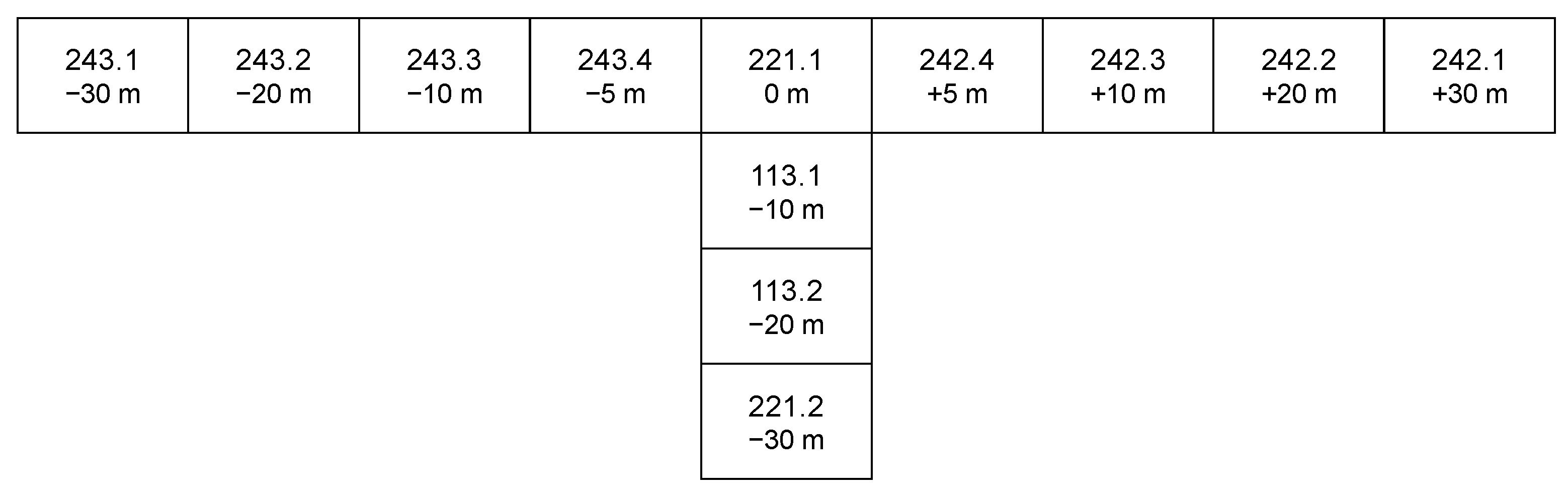
Figure 3 shows the twelve microphones arranged in a T shape. The microphones are overflown from the bottom (microphone 221.2) upward (microphone 221.1), whereas the cross stroke of the T captures lateral noise. The maximum distance to each side is 30 m, with microphone distances increasing outward. In the overflight direction, the 4 microphones are spaced at an equal distance of 10 m also starting 30 m before the cross stroke of the T.
The constant-speed propeller of the aircraft was operated in five distinct fixed pitch settings. The aircraft is not equipped with any means of measuring the blade pitch angle, therefore, the actual angle was measured on the ground, and then the whole flight performed in this setting. The pitch angle was measured at the outermost position of the blade in relation to the longitudinal axis of the aircraft. The mechanical low-pitch and high-pitch end stops can also be selected precisely in flight. For higher pitch angles, the take-off and climbing performance was no longer sufficient. Thus, the angle had to be adjusted throughout the flight for safety reasons. The 26.5° position was selected based on the time required to adjust the blade angle from the mechanical end stop to this setting on the ground. This leaves a few uncertainties: (i) precision in measuring time and stopping the blade adjustment and (ii) the potential influence of aerodynamic forces on the time needed for blade adjustment. Furthermore, not all combinations of airspeed and pitch angle are flyable in a safe manner because of overspeed or underspeed as well as poor climbing performance.
A few overflights had to be excluded from the final database due to the following factors. First of all, four overflights (two at maximum power and two with energy harvesting) were omitted due to their non-horizontal flight trajectories. Furthermore, some overflights were excluded due to waiting aircraft influencing noise measurements (two), due to an unstabilized overflight (one), or due to crickets sitting close to the microphone at the time of overflight (one, not already removed). Finally, all overflights at high altitudes were omitted from the database because of the limited emission angles and uncertainties due to atmospheric dampening. Ultimately, 22 overflights remained in the database.
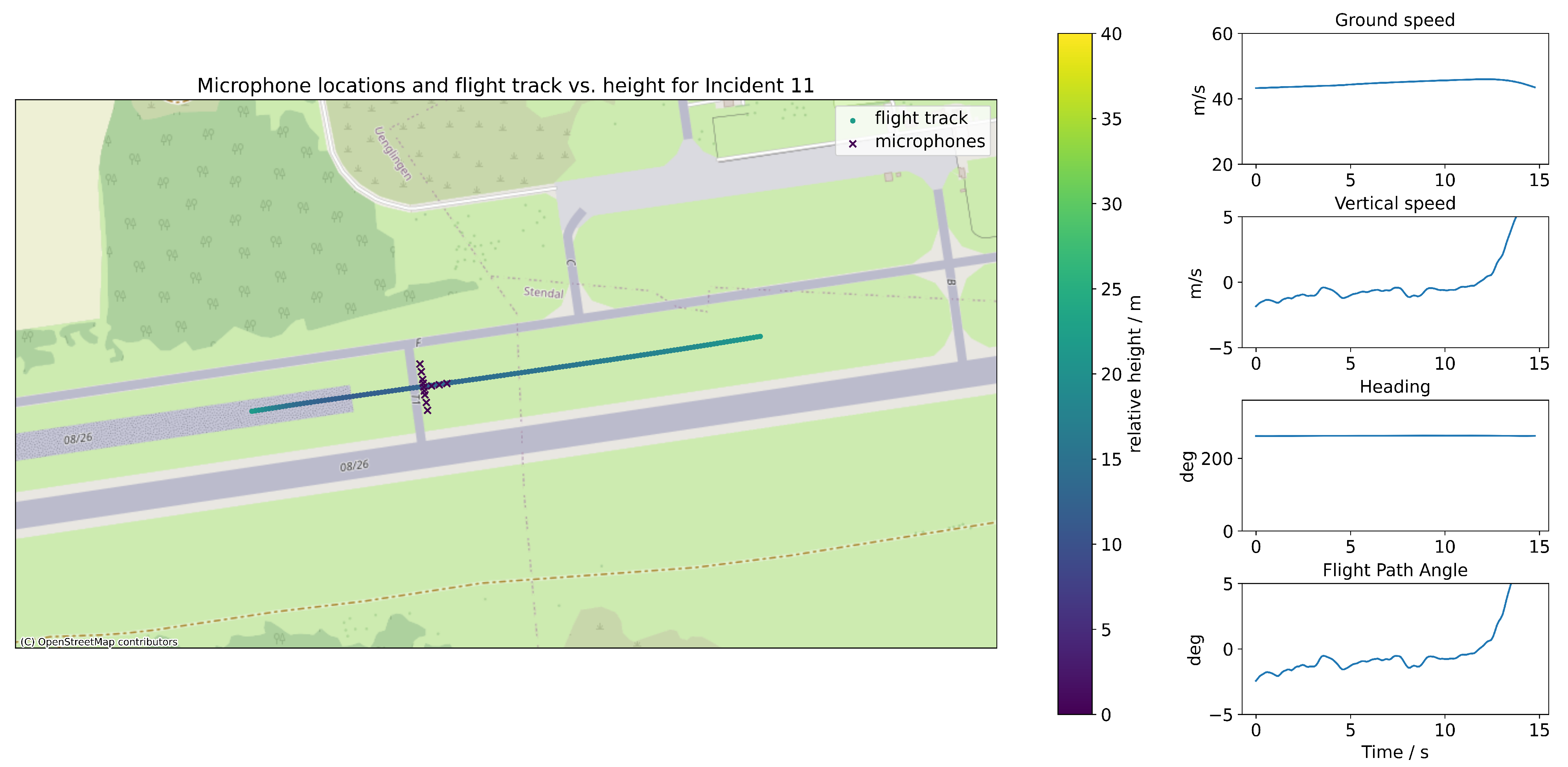
Figure 4 shows the ground track of incident 11 of the first recording. Each microphone is marked with an “x”, and the color map shows the height above ground of the aircraft. On the right-hand side, additional information is calculated based on the GPS fixes. The noticeable climb at the end is mostly not used within the evaluation or corrected for.
Every incident is processed in a similar manner using the evaluation routine of Eisenhut et al. [24], extended to include GPS-RTK measurements as well as background correction. In detail, the following steps are performed. Because the microphone is mounted above a metal base plate, the noise level is decreased by 6 dB to account for the total reflection [25]. Next, from each GPS fix in the log, the heading, ground speed and flight path angle can be calculated, assuming a slip-free flight. Optionally, a moving average can be selected for smoother results of this calculation. Based on heading and ground speed the relative velocity to each microphone can be calculated. This is used to remove the Doppler shift from the recording. In addition, the sign change of the relative velocity allows to identify the exact time of overflight of each microphone. Finally, considering the flight path of the aircraft and the travel time of sound, the delay time can be estimated, giving the position of the aircraft when the recorded sound was actually emitted. Based on this, the emission angles can be calculated, also correcting for any flight path angle.
For each overflight, 10 s of each microphone’s recording are evaluated. The frame size for the Fast Fourier Transforms (FFTs) is selected as 0.2 s, achieving 50% overlap and using a Hann window, resulting in 99 FFTs per overflight and microphone. Furthermore, for each overflight, a sample representing the background noise is manually selected. Depending on the background noise sample duration and selected window length, FFTs are calculated with the same settings as for the overflight itself. From all background FFTs, the Root Mean Square (RMS) is calculated, and this “mean” is removed from the overflight signal. Afterwards, together with the actual distance to each microphone at emission time, the sound pressure is corrected for geometrical spreading. Considering atmospheric damping with ISO 9613-1 [26] led to an overestimation of damping for higher distances and frequencies, resulting in unrealistic sound pressure at the specified reference distance. Thus, a correction for atmospheric damping was not included in the final data set.
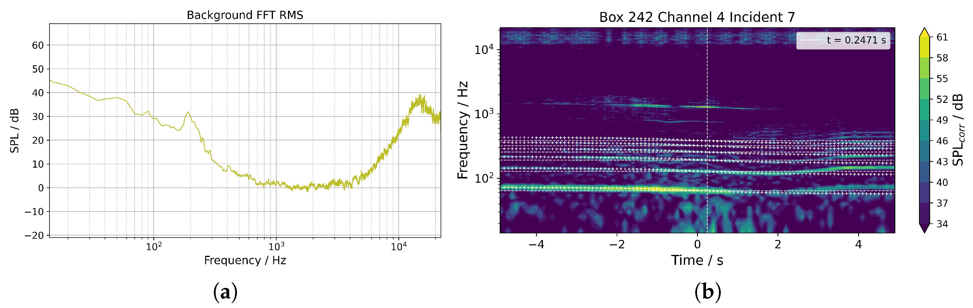
Figure 5 shows the influence of background noise on Sound Pressure Levels (SPLs) observed before and during some overflights, or, more specifically, the influence of crickets chirping close to the microphone. However, even on more distant microphones, this distinct signal was still visible in the graphs and audible in the recordings. On the left-hand side, Figure 5a shows the frequency of the background noise, with the increasing sound levels starting at roughly 4000 Hz. On the right, Figure 5b shows the background-corrected overflight signal, which has the following features: (i) periodic artifacts in higher-frequency regions due to the cricket can still be seen, and (ii) in the aircraft noise, especially at the Blade Passing Frequency (BPF), some information has been lost, e.g., around 2 s and the first BPF. In summary, this overflight is one of those that had to be excluded due to this environmental influence.
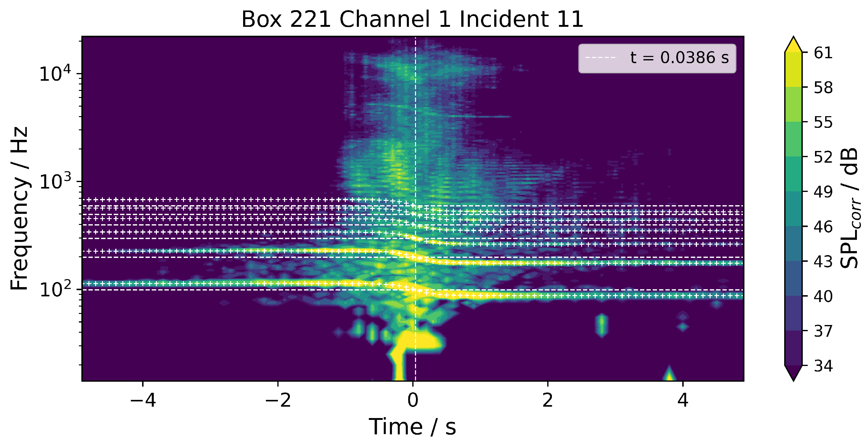
By examining the frequency over time, some plausibility checks can be performed before removing Doppler shift and applying geometrical spreading. Figure 6 shows that the ideal BPF (dashed horizontal line) and the exact time of the overflight (dashed vertical line, no Doppler shift) align with tonal noise components in the underlying experimental noise data. Furthermore, the calculated Doppler-shifted BPFs (drawn with “+” signs) based on the reported rotational speed of the propeller align well with the measured frequencies before and after the overflight. The first six multiples of the BPF are highlighted in the figure. The time on the upper right indicates the propagation time when the aircraft overflies the microphone and thus the sign of the relative velocity changes. In addition, the initiated increase in power (compare Figure 4) and thus RPM at fixed pitch is not yet reflected in the received audio signal, as there is no increase in frequency at the end of the signal. This is due to the propagation time necessary for the signal to be received by the microphones.
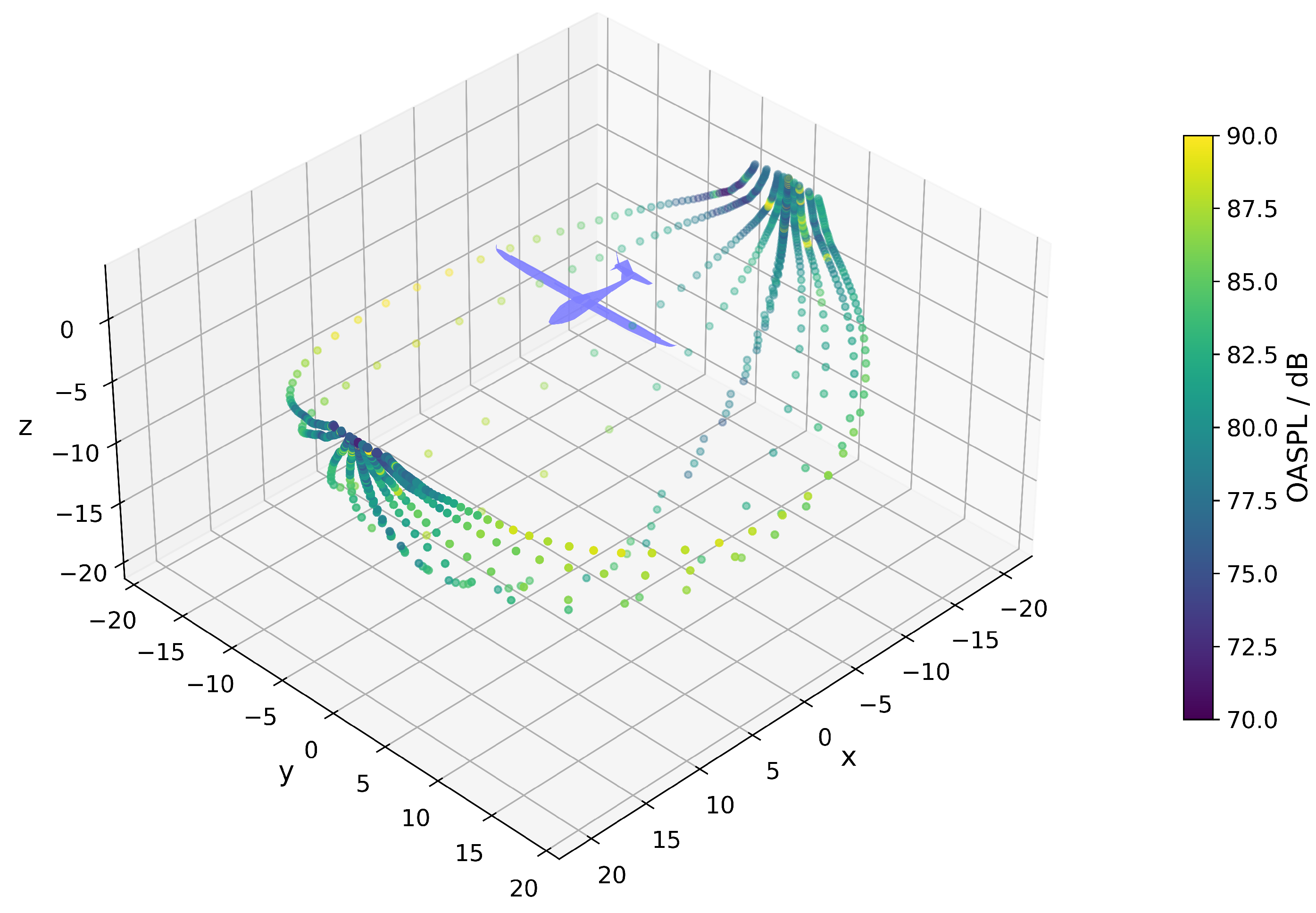
Overall, the hemisphere shown in Figure 7 can be created based on the overflight measurements and a reference radius of 20 m. The center microphones can be identified by the increased number of dots. In flight direction to the right, a local maximum is visible, while on the left a local minimum is visible. This can be explained by the vertical tail of the aircraft and the rotational direction of the propeller. Looking at the propeller from the front of the aircraft, the blades pass the vertical tail segment from left to right. This results in a reflection of airflow and noise on the vertical tail segment, leading to the local maximum on one side, and the shadowing causes a local minimum on the other side. Similarly, a shadowing effect by the horizontal tail segment is visible in some overflights.
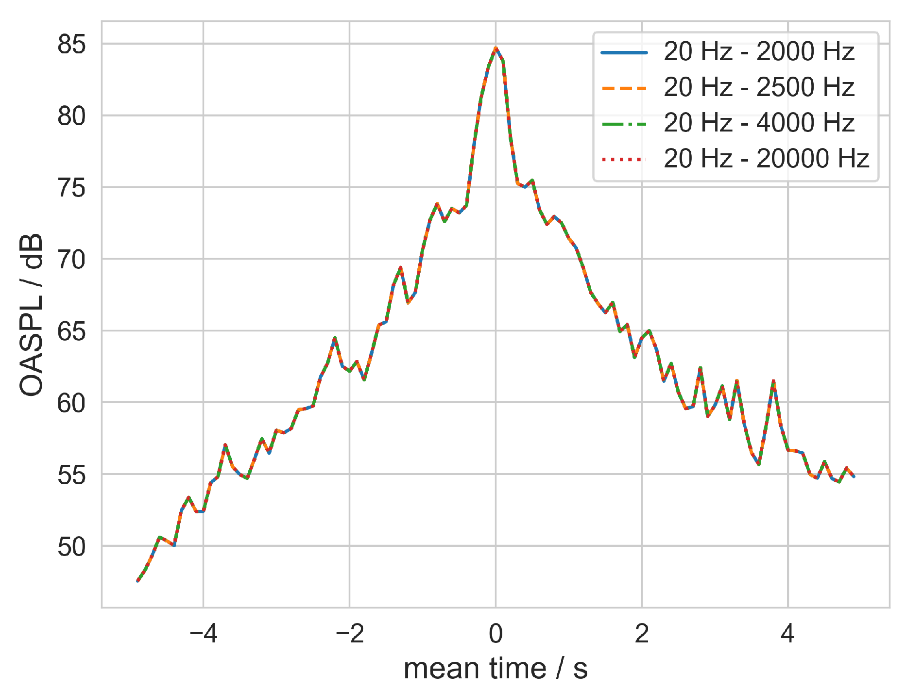
Finally, the calculation of the Overall Sound Pressure Level (OASPL) is limited to the one-third-octave bands d with center frequencies from 20 Hz up to 2500 Hz for the surrogate model. 20 Hz is the hearing limit of the human ear, and limiting the upper frequency can allow better future comparisons to currently performed simulations. This could allow a potential combination of experimental and simulative data in a future surrogate. Figure 8 shows that there is negligible influence on the OASPL over higher frequencies, therefore justifying the selection of the upper limit.

2.2. Machine Learning Approach for Fast Noise Prediction

For lower-dimensional input data or when creating a lookup table over a full grid is feasible, linear interpolation is a reasonable means within aircraft design. However, if there is no full grid, the interpolation relies on triangulation, which can be performed with SciPy’s LinearNDInterpolator (version 1.15.2 [27]). However, in the present case with 7 input parameters (dimensions), a total of 26 136 points, and a time complexity O ( n ( d / 2 ) ) (with n being the number of points and d the dimension), this is infeasible. Apart from time and memory constraints, the stability of the method was also an issue even in tests with reduced number of samples. Therefore, other methods need to be considered.
The present study investigates Linear Regression (LR), Support Vector Regression (SVR), Radial Basis Function (RBF) Interpolation, and Neural Networks (NNs). Python 3.12.9 is used together with SciPy 1.15.2 [27], scikit-learn 1.7.2 [28], and Keras 3.11.3 [29] with TensorFlow 2.20.0 [30]. While LR and SVR are build with scikit-learn, RBFInterpolator relies on SciPy, and NNs are built using Keras coupled with TensorFlow. Generally, an 80:20 split is used for training and test data. Hyperparameter optimization is performed with the help of GridSearchCV for 5-fold Cross-Validation (CV) for LR, SVR, and RBFInterpolator, while NN architectures are varied manually for different random seeds also using 5-fold CV. The loss function used here is Mean Squared Error (MSE). Only some models (those that perform best) are assessed on the test data. In addition to the MSE, the Mean Absolute Error (MAE) and R2 value as well as the Spearman r s and Kendall τ rank correlation coefficients are assessed.
In general, different scaling options are tested. These options include one with no scaling, as well as the following three scikit-learn scaling methods: (i) StandardScaler, (ii) PowerTransformer, and (iii) QuantileTransformer. Both the features and the targets of the data set are scaled with the same methods, but different scaling factors are used for each feature and target. However, no scaling and QuantileTransformer did not perform well compared to StandardScaler and PowerTransformer, which are similar. Unfortunately, the latter resulted in unfeasible results after inverse transformation in some cases. Due to this, only StandardScaler is assessed from this point onward.
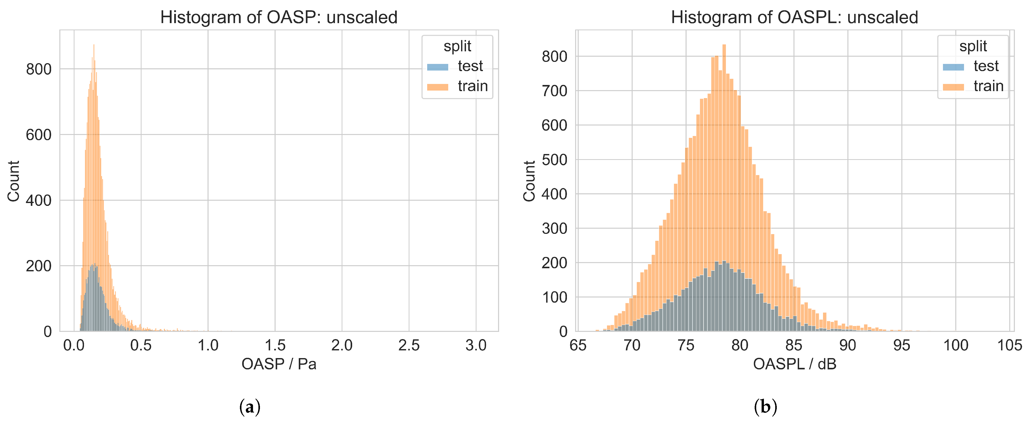
With regard to the targets, both options—predicting Overall Sound Pressure (OASP) and predicting OASPL—are tested at a radius of 20 m. However, a look at the histogram in Figure 9 already shows that the OASPL resembles a normal distribution more closely than the OASP.
For the faster models, training is performed on a workstation laptop with a 6-core Intel Core i7-9850H CPU, with 48 GB of RAM. For more time-consuming training, a node of the institute’s cluster was used. This has an AMD Epyc 9554 64-core CPU, 384 GB RAM, and an Nvidia L40s GPU with 48 GB RAM.

2.2.1. Single-Output Models

The single-output models are trained on six or seven features with a single output or target. The features—in other words, the inputs—are the direction of sound emission, either as spherical angles ( φ , θ ) or in Cartesian coordinates (x, y, z), as well as the velocity, rotational speed, propeller pitch angle, and power. Using the polar and azimuthal angles of spherical coordinates has the benefit of requiring one fewer feature; however, this poses the risk of singularity at the south pole as well as periodicity at 0 π and 2 π , which is not directly visible for the models. For Cartesian coordinates, both of these challenges are absent.
Looking at the underlying data, peaks in the histogram can be seen in front of and behind the aircraft (x ≈ ±20 m, y ≈ 0 m, and z ≈ 0 m or φ { 0 , π , 2 π } and θ π ). This clustering is visible in Figure 7. In addition, the remaining features (airspeed, rotational speed, propeller pitch angle, and power) have multiple peaks in the histogram, as the values are fixed throughout one overflight; one overflight provides 99 samples from each of 12 microphones, totaling 1188 points. The training set consists of 20 908 samples, and the test set consists of 5228 samples.

2.2.2. Multi-Output Models

The multi-output models share similar features with the single output models, but in contrast to adding the direction as a feature, the whole hemisphere is predicted at once. This allows smaller and faster models, at the risk of having an insufficient database consisting of only 22 overflights. These 22 flights must be split into training and test data as well, further reducing the number of samples available to train the models. Furthermore, each overflight consists of unique microphone locations that are not aligned with each other. The reasons for this are overflight velocity, variations in actual overflight height, and small deviations in lateral precision. Therefore, it is necessary to interpolate to a common representation. The steps performed are described in the following paragraphs.
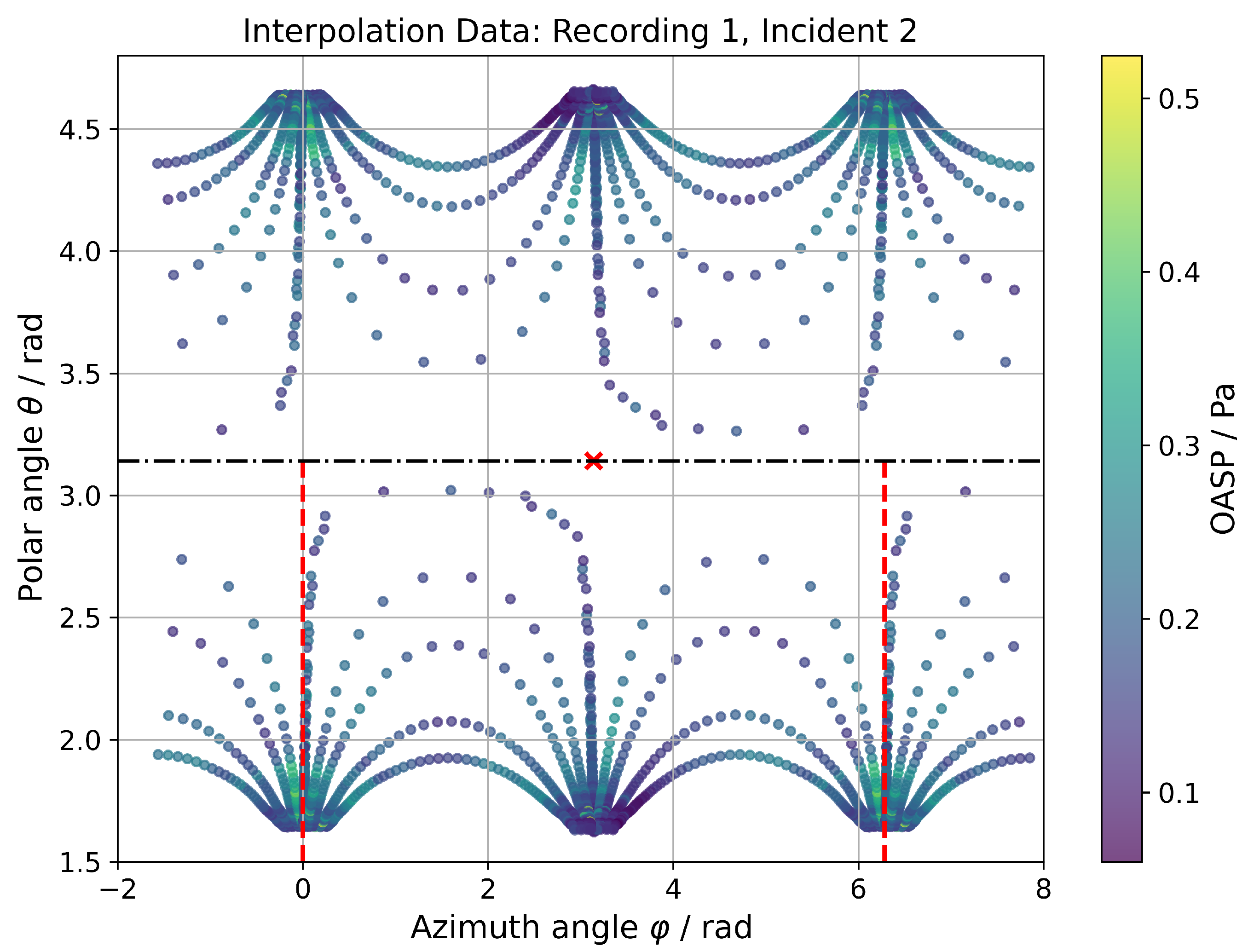
The first step consists of creating an interpolation surface for each overflight to interpolate the measured data points to a common selection of virtual microphones for all overflights. This is performed using a two-dimensional representation of the partial hemisphere, using azimuthal and polar angles, and the OASP at the radius of 20 m. Due to the singularity as well as periodicity already described in the previous section, the data are mirrored at φ = 0 π and φ = 2 π in the azimuthal direction, as well as reflected through φ = π in the polar θ direction. An example of the resulting data used by LinearNDInterpolator in SciPy is given in Figure 10. This case poses no difficulty in triangulation, as there is only a 2-dimensional space and the number of points is rather small.
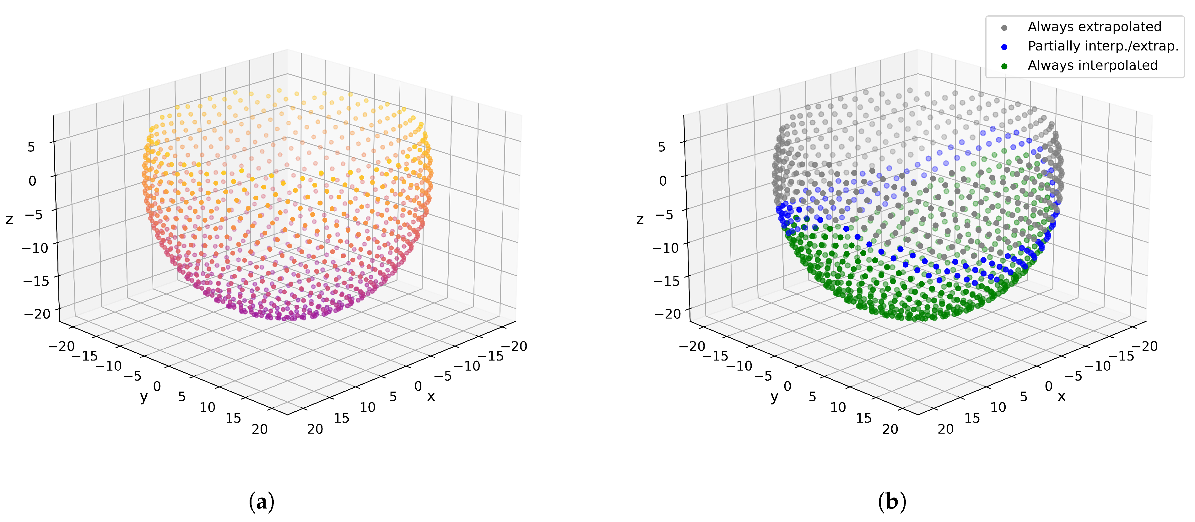
Having interpolation surfaces for all overflights, the next step is to select a common hemisphere. An equidistant grid of azimuthal and polar angles leads to a clustering or higher density at the poles; accordingly, a better option is a Fibonacci sphere [31]. Therefore, as a full grid is not necessary for the ML models, the second option is chosen. The selected sphere originally consists of 1493 points, but all points below θ = 70° are removed, resulting in a total of 1001 virtual microphones. This removal essentially cuts the top part of the sphere. Cutting 20° above the horizon is performed to ensure that the “horizontal emission” is captured while the aircraft is flying with a flight path angle at a maximum of 20°.
Figure 11a shows the resulting Fibonacci sphere. This is the same partial sphere that is used for a simulative database currently in creation. As the overflight measurements only partially cover these virtual microphones, all fully extrapolated points are marked and removed. Partially extrapolated points are also marked but kept. Figure 11b shows all these points combined across all overflights.
In the next step, the partially extrapolated points are filled using two approaches: first, singular value decomposition with the Python package fancyimpute (IterativeSVD) [32], and second, creation of an SVR model with scikit-learn. The goal of this approach is to create a model that can partially fit patterns within the data across all overflights. Therefore, this can improve the precision of these unknown values in comparison to a pure extrapolation from the individual overflight. In both cases, known data points are hidden from the training data (train), and with GridSearchCV, good models are searched, using the disclosed data for validation (val). The metric of the best SVR model is MSE val = 0.0301 in the scaled frame. This top-performing model is selected and retrained on the whole training set, reducing the loss on the test data to MSE test = 0.0293 in the scaled regime, or after scaling back to the original range to MSE test = 0.5546 . For comparison, the lowest MSEval for IterativeSVD is 12.070 (original). As the performance of the SVR model is better, the extrapolated values are replaced with the predictions of this model.
Overall, after removing the solely extrapolated microphones, 516 virtual microphones remain in the whole data set. This is more than an order of magnitude greater than the number of samples. In the next step, to reduce the dimensionality of the target, dimensionality reduction is performed using Principal Component Analysis (PCA). Depending on the total variance desired to be captured by all principal components, 5 (Var > 95%), 9 (Var > 98%), or 12 (Var > 99%) principal components result. Again, as more principal components are added, the risk of having too few available training samples increases. In total, the training set consists of 17 samples, and 5 samples remain for the test set.
In summary, the approach makes it possible to transform the uniquely measured overflight points to a common representation (virtual microphones from the Fibonacci sphere) and to reduce the dimensionality of the data. The general approach and transformation on the common representation can also be seen as a first step toward the ability to combine a simulative database with the experimental results to create a coupled surrogate model in the future. However, additional steps would be necessary to align the simulations with the experiments, e.g., considering atmospheric dampening. Furthermore, the aim of the simulations currently performed is to include non-stationary points, whereas the experimental overflights are performed as stationary horizontal overflights.

3. Results

This section will give an overview of the results for all investigated models grouped by the single-output and multi-output approaches. For each individual approach, various best models per setup are displayed; finally, an optimal configuration is down-selected, while overfitting is limited if necessary.

3.1. Single-Output Models

This first section covers the results of the single-output models. As described earlier, these use the direction as a trainable parameter and thus predict noise in relation to operational parameters and direction. The following approaches are used: LR, RBF interpolation, SVR, and NNs.

3.1.1. Linear Regression

LR is a simple methodology, and if it works reasonably well, the amount of effort required to set it up is small, as are the amounts of computational time and resources needed. Different models and hyperparameters are varied with scikit-learn’s GridSearchCV: plain LR, Lasso (L1 regularization), Ridge (L2 regularization), and ElasticNet (L1 and L2 regularization). The available hyperparameters for each model are varied over a wide range. Overall, as expected, the Cartesian coordinates resulted in better training and validation losses, as well as the usage of OASPL instead of OASP. The best models for each variant are summarized in Table 1. The table shows that all models achieve similar results, and the small difference between training and validation losses shows no sign of overfitting. However, the training and validation losses are quite high. Thus, the model is not capable of estimating the underlying data properly and learning all the non-linear features in the data. Therefore, no best model is selected.

3.1.2. RBF Interpolation

The performance of RBF interpolation is expected to be used as a baseline for other models. Again, the same two coordinate systems are used, and different available kernels and hyperparameters are tested. These are optimized using a wrapper function that makes the SciPy function compatible with GridSearchCV. The best models as defined by the lowest validation MSEs are given in Table 2. In all cases, using Cartesian coordinates and predicting OASPL produced the best results.
Most or all models in Table 2 show a tendency toward overfitting, as MSEtrain is substantially lower than MSEval. To select a model with lower overfitting, in addition to the validation loss (MSEval), the absolute difference between training and validation loss is also considered. Looking at the SVR in the next section, the limit is defined approximately as the gap for the best SVR model (<0.01). The resulting model that achieves the lowest MSEval while satisfying the gap constraint uses a quintic kernel. Its metrics are given in Table 3.
Furthermore, the Spearman r s and Kendall τ rank correlations are given in Table 4. This is helpful for conceptual aircraft design, as the rank correlation is a good measure of how well trends are maintained. The higher the score, the better the original order of the data is represented in the predictions, which entails a better chance of selecting the most promising configuration not only according to the model but also to the underlying data. The R2 score also gives a similar indication; however, this shows how far the predictions are from the perfect prediction without considering the actual ranks.

3.1.3. Support Vector Regression

For SVR, once again, GridSearchCV is used to find an optimal combination of model and hyperparameters. Different underlying functions, kernels, are used: linear, RBF, polynomial (degrees 2–6), and sigmoid. Table 5 shows the best-performing models based on the validation loss. In comparison to RBF interpolation, SVR has a lower tendency of overfitting. For the linear kernels, as with LR, it appears that the model is not able to capture the non-linearity and complexity of the underlying problem and that the sigmoid kernel is not working at all, with an MSE over 200 in scaled space. Further metrics for the best model with the lowest validation loss using the RBF kernel are given in Table 6 and Table 7.

3.1.4. Neural Network

The optimization and selection of a suitable model are performed manually with the assistance of scripts, due to the large parameter space and the infinite number of possible NN architectures. These scripts make it possible to calculate multiple architectures in parallel with various random seeds and CV folds. As the Cartesian coordinates and OASPL have proven reliable, this configuration alone will be investigated for the NN. Again, the reason is to reduce the complexity of the optimization task due to the infinite parameters available. Different numbers of hidden layers as well as neurons per layer, various dropout layers as well as rate, and L1/L2 regularization have been varied. The final model is selected based on the lowest validation loss while also considering the gap compared to the training data. This model is then assessed on the test data. Metrics of the selected NN model are given in Table 8 and Table 9. In contrast to RBF interpolation and SVR, no retraining based on the whole training set is possible with the NN, as the result is not deterministic. Therefore, a validation set is still necessary to select the epoch where minimal validation loss occurs.

3.2. Multi-Output Models

This section covers the same approaches again; however, due to the substantially lower performance, LR is not investigated further. For SVR and RBF, scikit-learns MultiOutputRegressor is used, resulting in distinct single-output models for each target. Thus, there is no connection between the different models or outputs, and hence, no potential influence between different targets is covered. In contrast, NNs work with multiple outputs from one model, and so potential influences of one target on another can be covered.
The results of RBF interpolation and SVR are not promising. The MSEtrain is substantially higher, and the models are also overfitted (deteriorating MSEval); to make matters worse, the R2 score is only slightly positive or sometimes even negative. In addition, the rank correlation ranges from almost -1 to 1 in some principal components. Therefore, the models are not usable. For SVR, it could be that the number of samples is too low to create a good model; the same may be true of the NN models. As expected, the number of neurons needed to create an overfitted model is reduced drastically, resulting in a simpler and faster model. However, as with the other two methods, there are principal components where the trends are not well covered. In general, models achieving an MSE close to those of the single-output models (MSE = 0.261) in training were drastically overfitted, with greater validation losses by a factor of four or more (MSE = 1.024). For models with reduced gaps between training (MSE = 0.956) and validation (MSE = 1.147) losses, the performance is still significantly lower than that of the single-output models. Therefore, due to their limited performance, the multi-output models are not investigated further.

4. Discussion

In general, the single-output models outperformed the multi-output models. This is attributable to the low number of samples and the higher complexity in the latter case. The PCA helps with this; however, there remain components where trends are not kept. Furthermore, in the single-output data, every overflight is part of the training data, as the direction is part of the input. Due to the selected training, validation and test splits, only some directions from some overflights are unknown for training. In the multi-output case, however, full overflights are unknown in training. However, even in training, metrics were not comparable to those of the single-output models. Therefore, this section discusses only three selected single-output models, namely, RBF interpolation, SVR, and NN, in further detail. Again, it must be noted that the RBF and SVR models are trained on the whole training set after CV, whereas the NN is only trained on 80% of the training set, as the remaining validation set is necessary to select the epoch with lowest validation loss.
As reflected by the metrics provided in Section 3.1, the SVR outperforms the RBF interpolation in all metrics. In this case, the interpolation is quite accurate, as there are many samples available. Regarding the NN, the metrics are even better, achieving reduced MSE and MAE values. Furthermore, the improved rank correlation values highlight that general trends are kept well. Only the R2 value is slightly lower. Specifically on the test data, the NN’s performance drops slightly more than that of the SVR, but the NN still prevails in all metrics. However, the SVR has the benefit that, for the test metric, the model can be retrained on the whole training set, whereas the NN still needs validation data to select the epoch with the lowest validation loss.
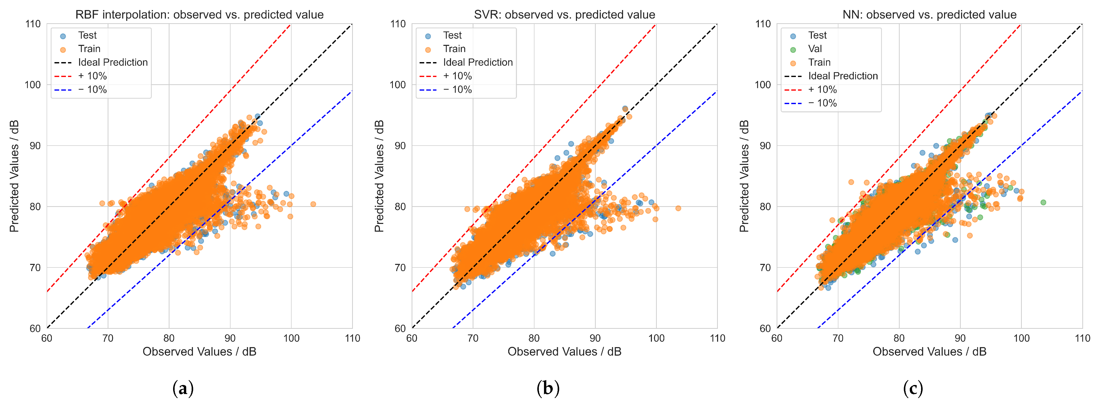
Figure 12 shows the performance of the three investigated single-output models and compares their predictions with the observed values. This underlines the impression given by the MSE and other metrics for each selected model. All three are similar in shape, with outliers in the same regions. Moving from best to worst, the NN in Figure 12c looks closer overall to the ideal prediction, which highlights the reduced MSE. The outlier region below the ideal line to the right seems slightly larger, emphasizing the lower R2 value. Next, the SVR in Figure 12b looks closer to the ideal, especially in the higher regime and close to the +10% line compared to the RBF interpolation in Figure 12a. In all cases, these outliers consist of points from all groups, i.e., the training, validation (if applicable), and test data. Furthermore, all these points share the common feature of being far forward or aft of the aircraft, where x ≈ ±20 m.
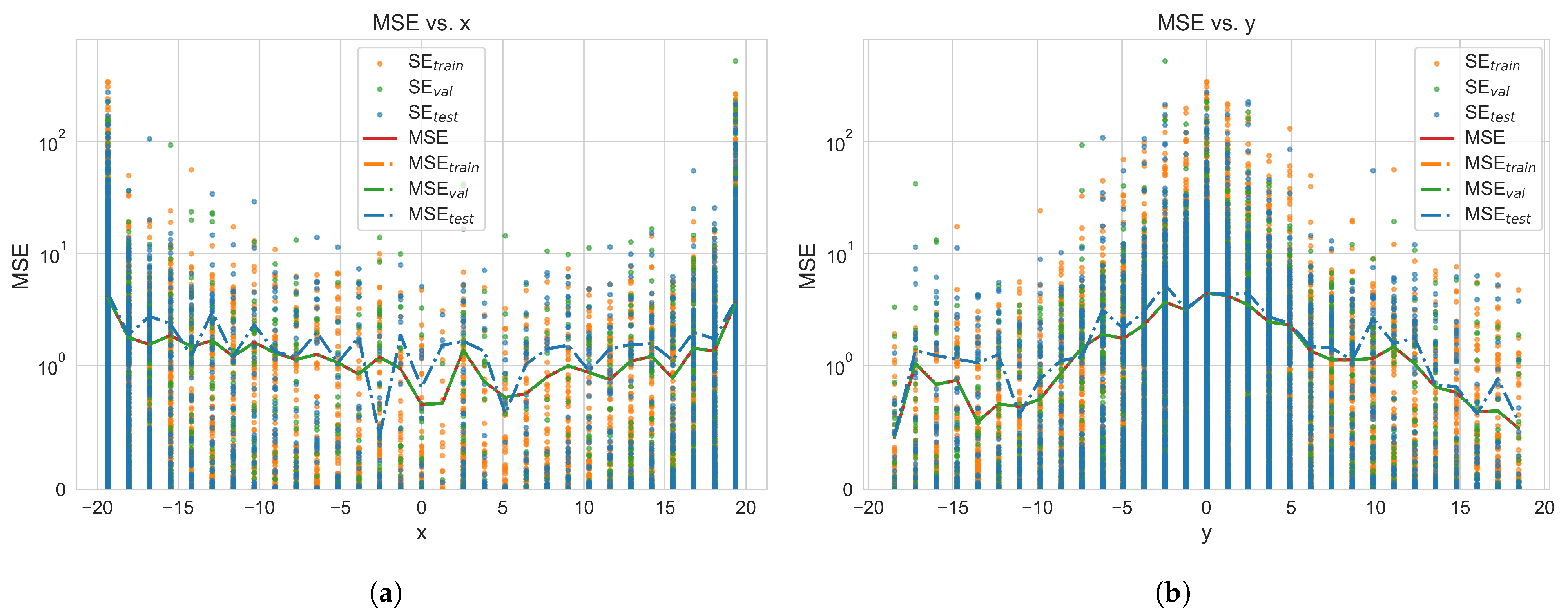
Figure 13 shows the variance or uncertainty (squared error and its mean) of the NN model against the x- and y-coordinates. The other two approaches lead to similar results. In front of and behind the aircraft (x ≈ ±20 m and y ≈ 0 m), we see the smallest differences between training, validation and test data, but the MSE is at its highest. The first observation can be explained by the number of samples in the region, which is at its highest due to the previously described clustering occurring in the overflight. The latter could be because the uncertainty in the experimental data is at a maximum because the distance from aircraft to microphone is at its highest. This leads to the highest atmospheric attenuation, which cannot be corrected for. Another point could be potential impacts due to a ground effect connected to shallow emission angles [33]. In contrast, directly below the aircraft (x ≈ 0 m and y ≈ ±20 m), the opposite effect occurs. First, the number of points is at its lowest, potentially increasing the gap between the training and test sets. Second, the experimental uncertainty is at its lowest due to the steep angle and low distance between aircraft and microphone; therefore, the MSE is at its minimum. In addition, the four center microphones lead to closely spaced, with varying noise levels. This impacts the overall prediction but can be more distinct where fewer observations are available in general, impacting, for example, the x ≈ 0 m region. Overall, all three models are suitable for the overall aircraft design, achieving good MSE and MAE values as well as rank correlations. The RBF and SVR models offer reasonably good results with almost no effort to set up, whereas the NN model offers improved metrics at the cost of an increased effort.
To account for these findings, two final NN models are trained using StandardScaler, OASPL and Cartesian coordinates. First, the impact of splitting training and test data is assessed by splitting whole overflights from the training data set. Here, the selection is performed manually to ensure good coverage of parameters varied in the overflights. Second, the potential uncertainty of more distant points is investigated by limiting any directions to 15° below the horizon. This leads to a total of 6126 samples: 4900 training samples and 1226 test samples for the standard splitting approach, and 4734 training samples (17 overflights) and 1392 test samples (5 overflights) for splitting over whole overflights. The same architecture is used for both approaches; however, the number of neurons per layer is reduced in contrast to the original NN due to the lower number of samples. Furthermore, the same random seed is used in both cases to eliminate any influence of randomness in initialization. The results are given in Table 10 and Table 11.
Table 10 and Table 11 show significantly improved accuracy for training and validation cases compared to the original NN model (see Section 3.1.4). Comparing the standard splitting and splitting by overflights for test data, we see the expected trends. The gap between training and validation is higher for the standard split, as all 22 overflights are part of these sets, increasing variance compared to the 17 overflights in the overflight split. For a similar reason, there is a larger drop in test metrics for the overflight split. These test samples are taken from the five overflights completely unknown to the model. However, the performance only drops towards the performance of the original NN model and not towards the values observed in the multi-output models., indicating that the bad performance of the multi-output models is due to other factors.
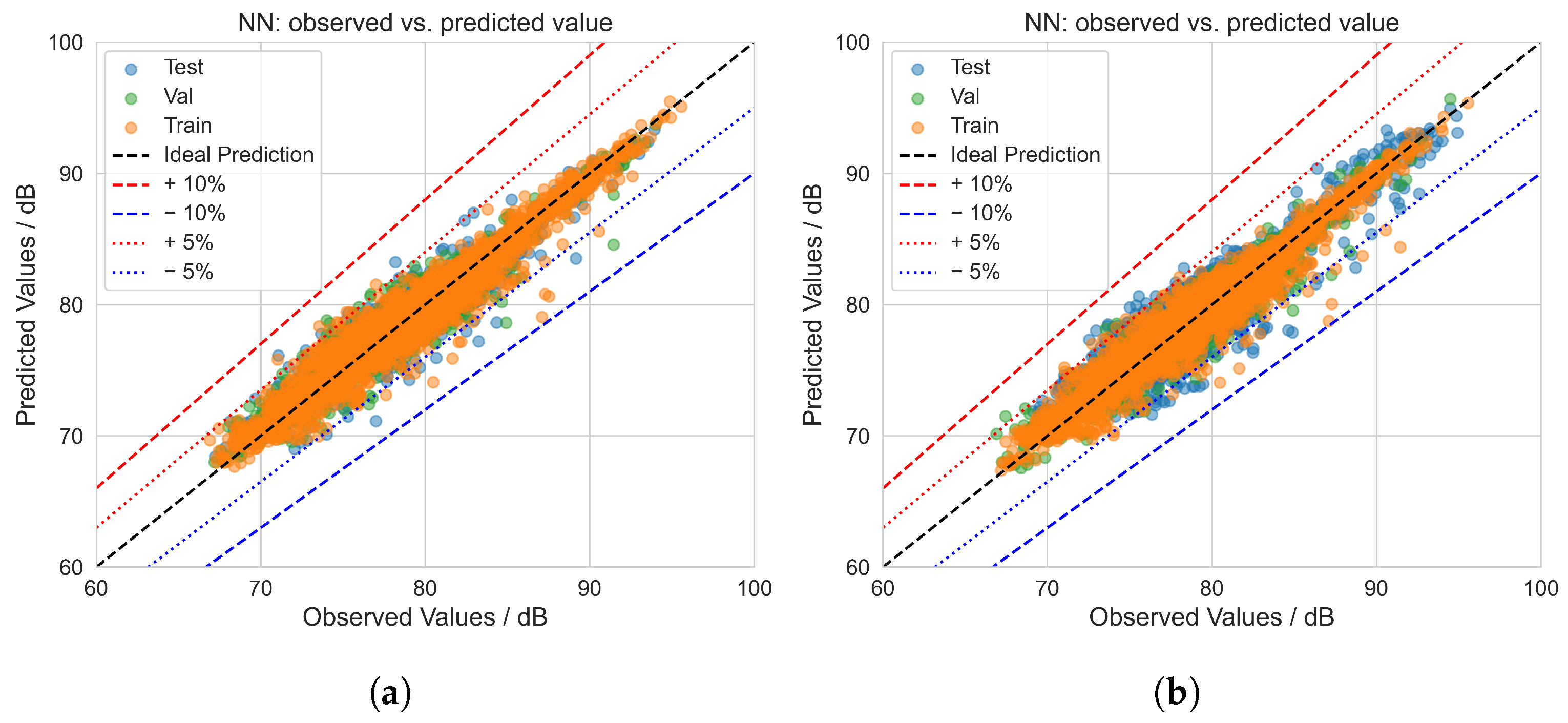
Figure 14 underlines the observed trends. Improved overall performance can be seen, as almost all points lie within the ±5% margins, whereas earlier many points were close to the ±10% margins. Furthermore, the disproportionate increase in MSEtest for the overflight split is underlined in Figure 14b, as more test samples (blue dots) are visible in the outer regions than in Figure 14a.
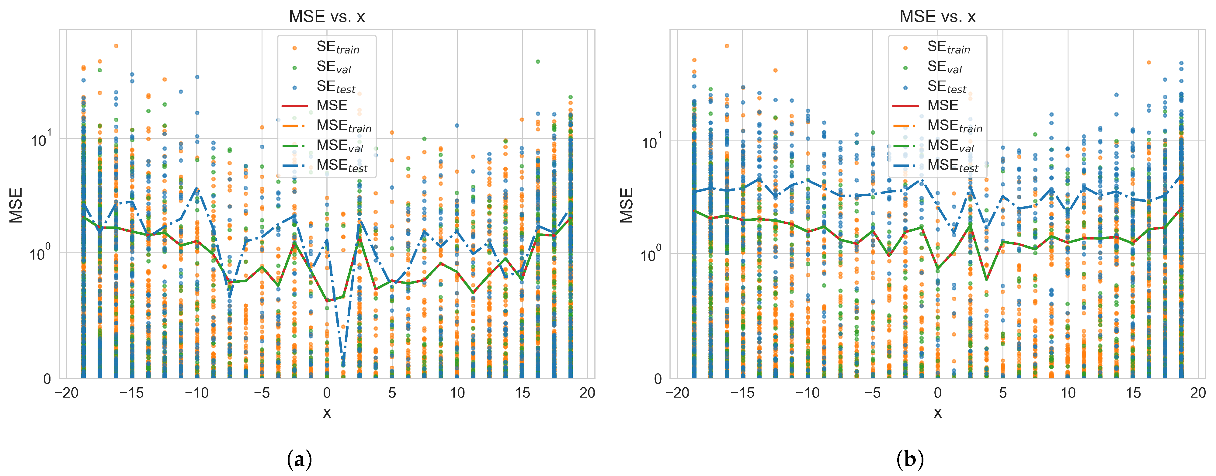
Looking at the x-coordinates again, Figure 15 shows that the overall loss is reduced compared to that of the original NN, which is in line with the previous findings. Furthermore, it highlights the differences between training, validation and test losses for the two splitting approaches. In Figure 15a, the test loss is closer to the training and, for one bin, even below it, whereas for the overflight split in Figure 15b, the test loss is always above the training and validation loss.
Overall, these final two models offer increased performance over previous models, further underscoring their suitability for overall aircraft design. Core metrics are drastically improved: the general accuracy (MSE, MAE and R2) is improved, and trends are even better reflected (Spearman r s and Kendall τ ).
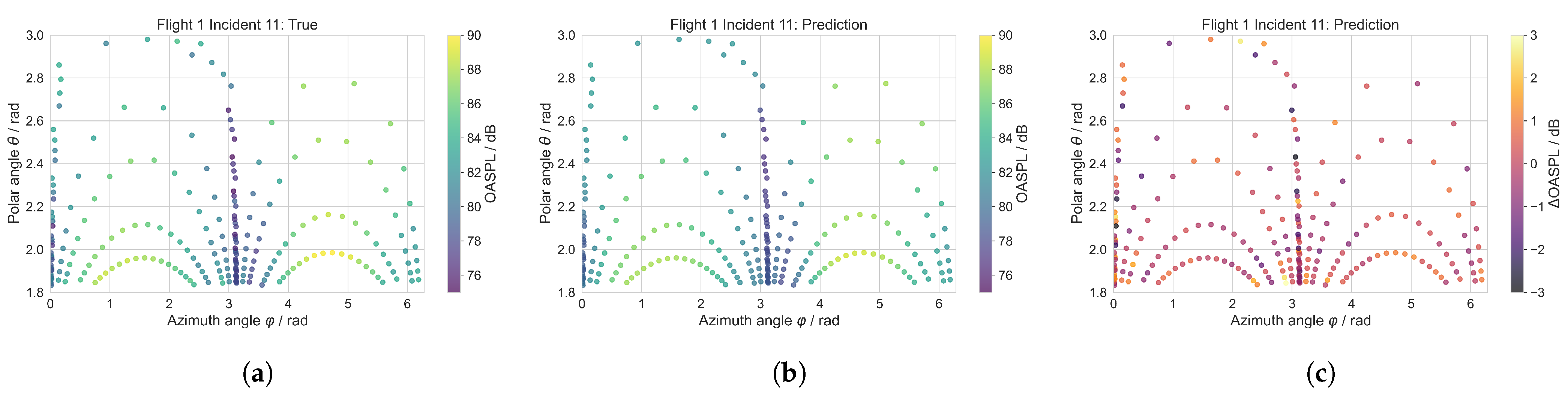
Finally, for one overflight (incident 11 of the first recording/flight), the accuracy of the standard split NN model is shown in Figure 16, while Figure 16a shows the true values from the experiment, Figure 16b shows the prediction of the NN, and Figure 16c shows the absolute differences between true and predicted values.
It can be seen that, especially for the four center microphones, the predictions vary the most regarding the ΔOASPL in Figure 16c. This is expected, as the experimental results have variations quite close together, whereas the predictions are “averaged” across these points. This tendency can also be observed in other overflights.

5. Conclusions and Outlook

This paper investigated the possibility of using ML approaches to estimate noise in overall aircraft design. The novel aspect of this study is that it bridges the gap to enable trade-offs between noise and performance in early design for the unconventional e-Genius. In this early stage, a fast prediction method covering the underlying physics is detrimental to any conceptual aircraft-level trade-off, where many options are assessed in a short time frame. Two approaches with different underlying methods have been investigated. The single-output models, which predicted only a single noise level depending on operational and directional parameters, outperformed the multi-output models which predicted a whole hemisphere at once.
When predicting a single output, the RBF interpolation achieves an MAE of 1.52 dB, while the SVR achieves 1.38 dB and the NN achieves 1.31 dB. This shows that NN and simpler models can estimate noise quite accurately. However, the amount of effort required is different. SVR can be set up and optimized with almost no effort. For RBF interpolation, a selection of an optimal model is necessary, reducing the gap between training and validation loss, to reduce overfitting tendencies. Depending on the desired accuracy and the time available for setup, RBF interpolation or SVR can be sufficient for the early design process, achieving good accuracy and maintaining trends. The additional manual effort to set up better-performing NNs might not be worthwhile in all cases. Furthermore, rank correlation shows good capabilities in terms of keeping necessary trends in the aircraft design process. This enables the confident selection of architectures or designs that not only appear to be the most promising but actually are the most promising out of the available options.
The multi-output models did not work properly for the task. Assessing different methods of splitting training and test data underlines the potential problem of not having enough samples available rather than the inevitable splitting of whole overflights in this approach. Finally, this study showed that limiting the emission angle further by removing points with the highest uncertainty from the experimental data improves the performance of the NN models. Here, an MAE in the region of 1 dB is possible for completely unknown data, also achieving high rank correlations and R2 values above 0.9.
The next steps include creating a model based on simulation data, which would have several benefits over flight tests: (i) geometric adaptation is possible; (ii) no flying aircraft is required; and (iii) the microphones are always at the same position, with no variance in overflight height or lateral deviation. This database will consist of non-stationary flight points and will allow some geometrical adjustments of the underlying aircraft concept. If necessary, frequency-based models could also be trained by increasing the model dimensionality or number of models, allowing to assess the approach for frequency bands as well. In addition, we plan to enable aircraft-level trade-offs by adding the models to an aircraft design toolbox, enabling the prediction of certification metrics and more. Furthermore, comparisons to existing methods in the toolbox could be performed.

Author Contributions

Conceptualization, D.E.; methodology, D.E.; software, D.E.; validation, D.E.; formal analysis, D.E.; investigation, D.E.; resources, D.E.; data curation, D.E.; writing—original draft preparation, D.E.; writing—review and editing, D.E. and A.S.; visualization, D.E.; supervision, A.S.; project administration, D.E.; funding acquisition, D.E. All authors have read and agreed to the published version of the manuscript.

Funding

This Project is supported by the Federal Ministry for Economic Affairs and Climate Action (BMWK) on the basis of a decision by the German Bundestag. Grant ID: KK5102509SY3.

Data Availability Statement

All relevant data are included as figures or tables in the main article. Further inquiries can be directed to the corresponding author.

Acknowledgments

The authors would like to thank their project partners for engaging them in fruitful discussions. The authors also express their gratitude to the Institute of Aerodynamics and Gas Dynamics at the University of Stuttgart for providing the noise measurement equipment. Finally, the authors extend special thanks to their colleague Andreas Bender for providing support during the noise measurement campaign and data evaluation.

Conflicts of Interest

The authors declare no conflicts of interest.

Abbreviations

The following abbreviations are used in this manuscript:
BPFBlade Passing Frequency
CFDComputational Fluid Dynamics
CVCross-Validation
DEPDistributed Electric Propulsion
FFTFast Fourier Transform
GPSGlobal Positioning System
LRLinear Regression
MAEMean Absolute Error
MLMachine Learning
MSEMean Squared Error
NNNeural Network
PCAPrincipal Component Analysis
RBFRadial Basis Function
RMSRoot Mean Square
RTKReal-Time Kinematics
SPLSound Pressure Level
SVRSupport Vector Regression
OASPOverall Sound Pressure
OASPLOverall Sound Pressure Level

References

  1. European Commission Directorate General for Research and Innovation; European Commission Directorate General for Mobility and Transport. Flightpath 2050 Europe’s Vision for Aviation; Publications Office: Luxembourg, 2011. [Google Scholar]
  2. European Commission; Directorate General for Research and Innovation. Fly the Green Deal: Europe’s Vision for Sustainable Aviation; Publications Office: Luxembourg, 2022. [Google Scholar]
  3. Electra.Aero. Electra.Aero|Electra Completes World’s First Hybrid-Electric eSTOL Aircraft Flight. 2023. Available online: https://www.electra.aero/news/worlds-first-hybrid-electric-estol-flight (accessed on 23 February 2026).
  4. Electra.Aero. Electra.Aero|Electra Reveals Design for EL9 Ultra Short Hybrid-Electric Aircraft. 2024. Available online: https://www.electra.aero/news/electra-reveals-design-for-el9-ultra-short-hybrid-electric-aircraft (accessed on 23 February 2026).
  5. Zawodny, N.S.; Boyd, D.D.; Nark, D.M. Aerodynamic and Acoustic Interactions Associated with Inboard Propeller-Wing Configurations. In Proceedings of the AIAA Scitech 2021 Forum, Virtual Event, 11–15, 19–21 January 2021. [Google Scholar] [CrossRef]
  6. Wickersheim, R.; Keßler, M.; Sembowski, J.; Bongen, D.; Gomes, J. Numerical Investigation and Validation of Noise Sources of a Distributed Propulsion System. AIAA J. 2025, 63, 1418–1430. [Google Scholar] [CrossRef]
  7. Wickersheim, R.; Keßler, M.; Krämer, E. Numerical Identification of Tonal Noise Sources and Comparison With Fly-Over Measurements of a Distributed Electric Propulsion-Flight Demonstrator. In Proceedings of the AIAA SCITECH 2025 Forum, Orlando, FL, USA, 6–10 January 2025. [Google Scholar] [CrossRef]
  8. International Civil Aviation Organization. Annex 16 Environmental Protection Volume I—Aircraft Noise, 8th ed.; International Civil Aviation Organization: Montreal, QC, Canada, 2017. [Google Scholar]
  9. Bertsch, L.; Dobrzynski, W.; Guérin, S. Tool Development for Low-Noise Aircraft Design. J. Aircr. 2010, 47, 694–699. [Google Scholar] [CrossRef]
  10. Koch, H.M. Reduction of Aircraft Noise by Wing Design and Add-On Technologies. Ph.D. Thesis, TU Braunschweig, Göttingen, Germany, 2021. [Google Scholar]
  11. Le Clainche, S.; Ferrer, E.; Gibson, S.; Cross, E.; Parente, A.; Vinuesa, R. Improving Aircraft Performance Using Machine Learning: A Review. Aerosp. Sci. Technol. 2023, 138, 108354. [Google Scholar] [CrossRef]
  12. Brunton, S.L.; Nathan Kutz, J.; Manohar, K.; Aravkin, A.Y.; Morgansen, K.; Klemisch, J.; Goebel, N.; Buttrick, J.; Poskin, J.; Blom-Schieber, A.W.; et al. Data-Driven Aerospace Engineering: Reframing the Industry with Machine Learning. AIAA J. 2021, 59, 2820–2847. [Google Scholar] [CrossRef]
  13. Dong, Y.; Tao, J.; Zhang, Y.; Lin, W.; Ai, J. Deep Learning in Aircraft Design, Dynamics, and Control: Review and Prospects. IEEE Trans. Aerosp. Electron. Syst. 2021, 57, 2346–2368. [Google Scholar] [CrossRef]
  14. Li, J.; Du, X.; Martins, J.R.R.A. Machine Learning in Aerodynamic Shape Optimization. Prog. Aerosp. Sci. 2022, 134, 100849. [Google Scholar] [CrossRef]
  15. Bianco, M.J.; Gerstoft, P.; Traer, J.; Ozanich, E.; Roch, M.A.; Gannot, S.; Deledalle, C.A. Machine Learning in Acoustics: Theory and Applications. J. Acoust. Soc. Am. 2019, 146, 3590–3628. [Google Scholar] [CrossRef] [PubMed]
  16. Amirsalari, B.; Rocha, J. Recent Advances in Airfoil Self-Noise Passive Reduction. Aerospace 2023, 10, 791. [Google Scholar] [CrossRef]
  17. Poggi, C.; Rossetti, M.; Bernardini, G.; Iemma, U.; Andolfi, C.; Milano, C.; Gennaretti, M. Surrogate Models for Predicting Noise Emission and Aerodynamic Performance of Propellers. Aerosp. Sci. Technol. 2022, 125, 107016. [Google Scholar] [CrossRef]
  18. Poggi, C.; Rossetti, M.; Serafini, J.; Bernardini, G.; Gennaretti, M.; Iemma, U. Neural Network Meta–Modelling for an Efficient Prediction of Propeller Array Acoustic Signature. Aerosp. Sci. Technol. 2022, 130, 107910. [Google Scholar] [CrossRef]
  19. Thurman, C.; Zawodny, N. Aeroacoustic Characterization of Optimum Hovering Rotors Using Artificial Neural Networks. In Proceedings of the Vertical Flight Society 77th Annual Forum, Virtual Conference, 10–14 May 2021; pp. 1–10. [Google Scholar] [CrossRef]
  20. Manghnani, J.; Ewert, R.; Delfs, J.W. Predicting Propeller Tonal Noise with AI Trained First-Principle Models: A Novel Methodology. In Proceedings of the DAS|DAGA 2025, Copenhagen, Denmark, 17–20 March 2025. [Google Scholar]
  21. Manghnani, J.; Domogalla, V.; Ewert, R.; Bertsch, L.; Delfs, J.W. A First Principle Based Approach for Prediction of Tonal Noise From Isolated and Installed Propeller. In Proceedings of the 30th AIAA/CEAS Aeroacoustics Conference (2024), Rome, Italy, 4–7 June 2024. [Google Scholar] [CrossRef]
  22. Manghnani, J.; Ewert, R.; Delfs, J. Towards Data-Driven Aeroacoustic Modeling to Predict Propeller Installation Noise: A First-Principle Based Approach. In Proceedings of the AIAA Aviation Forum and Ascend 2025, Las Vegas, NV, USA, 21–25 July 2025. [Google Scholar] [CrossRef]
  23. Institute of Aircraft Design, University of Stuttgart. E-Genius Homepage. Available online: https://www.ifb.uni-stuttgart.de/en/research/aircraftdesign/mannedaircraft/e-genius/ (accessed on 24 February 2026).
  24. Eisenhut, D.; Bender, A.; Strohmayer, A. Overflight Noise Measurements of a Crewed All-Electric Flying Demonstrator. In Proceedings of the 11th European Conference for Aeronautics and Aerospace Sciences (EUCASS), Roma, Italy, 30 June–4 July 2025. [Google Scholar] [CrossRef]
  25. DIN 45684-2:2015-12; Akustik_—Ermittlung von Fluggeräuschimmissionen an Landeplätzen_—Teil_2: Bestimmung Akustischer und Flugbetrieblicher Kenngrößen; Text Deutsch und Englisch. German Institute for Standardisation: Berlin, Germany, 2015. [CrossRef]
  26. ISO 9613-1; Acoustics—Attenuation of Sound during Propagation Outdoors. ISO: Geneva, Switzerland, 1993.
  27. Virtanen, P.; Gommers, R.; Oliphant, T.E.; Haberland, M.; Reddy, T.; Cournapeau, D.; Burovski, E.; Peterson, P.; Weckesser, W.; Bright, J.; et al. SciPy 1.0: Fundamental Algorithms for Scientific Computing in Python. Nat. Methods 2020, 17, 261–272. [Google Scholar] [CrossRef] [PubMed]
  28. Pedregosa, F.; Varoquaux, G.; Gramfort, A.; Michel, V.; Thirion, B.; Grisel, O.; Blondel, M.; Prettenhofer, P.; Weiss, R.; Dubourg, V.; et al. Scikit-Learn: Machine Learning in Python. J. Mach. Learn. Res. 2011, 12, 2825–2830. [Google Scholar]
  29. Chollet, F. Keras. 2015. Available online: https://keras.io (accessed on 23 February 2026).
  30. Abadi, M.; Agarwal, A.; Barham, P.; Brevdo, E.; Chen, Z.; Citro, C.; Corrado, G.S.; Davis, A.; Dean, J.; Devin, M.; et al. TensorFlow: Large-Scale Machine Learning on Heterogeneous Distributed Systems. arXiv 2016, arXiv:1603.04467. [Google Scholar]
  31. González, Á. Measurement of Areas on a Sphere Using Fibonacci and Latitude-Longitude Lattices. Math. Geosci. 2010, 42, 49–64. [Google Scholar] [CrossRef]
  32. Rubinsteyn, A.; Feldman, S. Fancyimpute: An Imputation Library for Python. 2016. Available online: https://github.com/iskandr/fancyimpute (accessed on 23 February 2026).
  33. Feldhusen-Hoffmann, A.; Bertsch, L.; Pott-Pollenske, M.; Domogalla, V.; Kreienfeld, M.; Doerge, N. Noise and Local Pollutants of Small Aircraft: Overview of Simulation Activities and of the First Flight Test within the DLR Project L2 INK. In Proceedings of the AIAA AVIATION 2023 Forum, San Diego, CA, USA and Online, 12–16 June 2023. [Google Scholar] [CrossRef]
Figure 1. e-Genius in its fully battery-electric configuration. Photographed by Tobias Barth.
Aerospace 13 00292 g001
Figure 2. Noise measurement setup: microphone mounted upside down on a ground plate. In the background, one of the measurement boxes can be seen.
Aerospace 13 00292 g002
Figure 3. Noise measurement setup: microphone arrangement (box.channel), including relative distances to the center microphone.
Aerospace 13 00292 g003
Figure 4. Example ground track, derived from incident 11, recording 1. Microphone positions are marked as x, and the height above the center microphone is represented by the color of the track. At the end of the sequence, roughly at time 12.5 s, the power is increased and a climb is initiated, as can be seen in the vertical speed and flight path angle.
Aerospace 13 00292 g004
Figure 5. Influence of crickets on the noise measurement. (a) RMS of all FFTs performed for one background noise excerpt. There is a very distinct increase in SPL beginning roughly at 4000 Hz. (b) During the overflight, the chirping of the cricket is still seen in the FFT graph at high frequencies after correcting for the background signal, where SPLcorr is the background-corrected SPL. Furthermore, aircraft noise features are partially removed.
Aerospace 13 00292 g005
Figure 6. FFT over time for the center microphone (221.1) for the incident 11 of the first flight. Time 0 s is exactly when the aircraft overflies the microphone. Taking into account the propagation time (speed of sound, t = 0.0386 s), the vertical dashed line marks the overflight time as recorded by the microphone. The horizontal dashed lines mark the ideal first six BPFs without a Doppler shift. Furthermore, the + signs mark the calculated Doppler-shifted first six BPFs based on the relative velocity from the GPS. SPLcorr is the background-corrected SPL.
Aerospace 13 00292 g006
Figure 7. OASPL hemisphere extracted from all twelve microphones and 99 FFTs for incident 11, flight 1, given relative to a reference radius of 20 m. The orientation of the aircraft is given by the transparent model drawn to scale, with the center of the hemisphere assumed at x = 25% Mean Aerodynamic Chord on the longitudinal axis.
Aerospace 13 00292 g007
Figure 8. OASPL over one overflight (incident 11 of recording 1) for different one-third-octave band upper limits. The influence of higher frequencies on the OASPL is negligible, as can be seen by the coinciding lines.
Aerospace 13 00292 g008
Figure 9. Comparison of the histograms of OASP and OASPL for all overflights in the data set. Test data in blue and training data in orange. (a) Histogram of unscaled OASP in Pa, with minimum 0.0428 Pa and maximum 3.018 Pa. (b) Histogram of unscaled OASPL in dB, with minimum 66.61 dB and maximum 103.58 dB.
Aerospace 13 00292 g009
Figure 10. Resulting data after mirroring and reflection to account for singularity and periodicity for one exemplary overflight. The original data and interpolations are in the range φ = [ 0 , 2 π ] and θ = [ 0 , π ] . Mirroring for periodicity is shown with the red dashed lines, and the point reflection due to the singularity is shown by the x marker. In addition, the dash–dot line is shown to highlight the singularity.
Aerospace 13 00292 g010
Figure 11. Fibonacci sphere and the (partially) extrapolated points. (a) Virtual microphones on the Fibonacci sphere, cut 20° above the horizon. The color gradient highlights the z-value. (b) Always-extrapolated values (gray), partially interpolated/extrapolated values (blue), and always-interpolated values (green) on the Fibonacci sphere based on all overflights.
Aerospace 13 00292 g011
Figure 12. Predicted values versus observed values for the RBF interpolation, SVR, and NN models. Training data are shown in orange, test data in blue, and NN validation data in green. The black dashed line is the ideal prediction, red is +10% and blue is −10%. Sub-figures: (a) RBF interpolation, (b) SVR, and (c) NN.
Aerospace 13 00292 g012
Figure 13. The graphs show the squared error (SE) and its mean for bins across the x- and y-coordinates. The results for the NN model are the ones displayed; however, the other approaches lead to similar results. Sub-figures: (a) MSE vs. x-coordinate, and (b) MSE vs. y-coordinate.
Aerospace 13 00292 g013
Figure 14. Predicted values versus observed values for both NN splitting variants. Training data are shown in orange, validation data in green, and test data in blue. The black dashed line is the ideal prediction, whereas red is +10% or +5% and blue is −10% or −5%. Sub-figure: (a) standard splitting approach, (b) splitting by overflight.
Aerospace 13 00292 g014
Figure 15. The figures show the squared error (SE) and its mean for bins over the x-coordinates for both splitting options. The sub figure (a) is for the standard split, and (b) is for the overflight split.
Aerospace 13 00292 g015
Figure 16. Overview of the experimental results, predictions by the standard split NN, and absolute ΔOASPL. Sub-figures: (a) experimental results, (b) predictions, (c) ΔOASPL.
Aerospace 13 00292 g016
Table 1. Metrics of the LR models with the lowest MSEval for each model, where MSE is given in the scaled frame and MSEdB is given as OASPL in dB. All best models are with Cartesian coordinates and OASPL for training.
ModelMSEtrainMSEvalMSEdB, trainMSEdB, val
Lin. Reg.0.6019220.6026159.9465259.957974
Lasso0.6019220.6026159.9465279.957974
Ridge0.6019240.6026099.9465549.957883
ElasticNet0.6019270.6026099.9466059.957875
Table 2. Metrics of the RBF interpolation model with the lowest MSEdB, val for each kernel. All models are based on Cartesian coordinates and OASPL.
KernelMSEtrainMSEvalMSEdB, trainMSEdB, val
Linear0.0890.2001.4723.307
TPS 10.1450.2042.3993.367
Cubic0.1420.2082.3513.445
Quintic0.1690.2212.7903.656
MQ 20.1370.2022.2703.339
IQ 30.1750.2242.8963.698
IMQ 40.0910.2181.5073.598
Gaussian0.2080.2313.4293.825
1 thin plate spline 2 multiquadric 3 inverse quadratic 4 inverse multiquadric.
Table 3. Metrics of the selected RBF interpolator model (Cartesian coordinates, quintic kernel, StandardScaler, and OASPL). Training and validation metrics are the mean of all CV folds. All test metrics are calculated for a model retrained on the whole training set, resulting in improvement over validation metrics.
MSEtrainMSEvalR2trainR2valMSEtestMAEtestR2test
Scaled0.2730.2780.7270.7220.2720.3730.719
OASPL4.5144.5950.7270.7224.4951.5160.719
Table 4. Rank correlations of the selected RBF interpolator model (Cartesian coordinates, quintic kernel, StandardScaler, and OASPL) calculated on the final model, where the training set is the whole set without any validation data. Rank correlation is unaffected by scaling.
r s , train r s , test r s , combined τ train τ test τ combined
0.8530.8420.8510.6730.6630.671
Table 5. Metrics of the SVR model with the lowest MSEdB, val for each kernel. All models are based on Cartesian coordinates and OASPL.
KernelMSEtrainMSEvalMSEdB, trainMSEdB, val
Linear0.6030.6039.9589.970
RBF0.2410.2503.9854.135
2nd Poly.0.4020.4036.6356.658
3rd Poly.0.3230.3265.3395.387
4th Poly.0.2810.2854.6424.709
5th Poly.0.2670.2734.4154.505
6th Poly.0.2570.2654.2534.371
Table 6. Metrics of the selected SVR model (Cartesian coordinates, RBF kernel, StandardScaler, and OASPL). Training and validation metrics are the mean of all CV folds. All test metrics are calculated with a model retrained on the whole training set, resulting in improvement over validation metrics.
MSEtrainMSEvalR2trainR2valMSEtestMAEtestR2test
scaled0.2410.2500.7590.7500.2470.3400.745
OASPL3.9854.1350.7590.7504.0741.3800.745
Table 7. Rank correlations of the selected SVR model (Cartesian coordinates, RBF kernel, StandardScaler, and OASPL) calculated on the final model, where the training set is the whole set without any validation data. Rank correlation is unaffected by scaling.
r s , train r s , test r s , combined τ train τ test τ combined
0.8750.8620.8720.7040.6890.701
Table 8. Metrics of the selected NN model. Training and validation metrics are given at the epoch where the minimal validation loss occurs. Test metrics are calculated on the same model.
MSEtrainMSEvalR2trainR2valMSEtestMAEtestR2test
Scaled0.1870.2020.7620.7410.2130.3210.720
OASPL3.0953.3370.7620.7413.5161.3060.720
Table 9. Rank correlations of the selected NN model for the final model; training metrics are given for the full training set (including validation data). Rank correlation is unaffected by scaling.
r s , train r s , test r s , combined τ train τ test τ combined
0.9010.8810.8970.7380.7130.733
Table 10. Metrics of the NN model with standard split. Training and validation metrics are given at the epoch where the minimal validation loss occurs.
MetricFrameTrainValTest
MSEScaled0.0570.0840.090
OASPL1.1921.7501.880
MAEscaled0.1740.2130.225
OASPL0.7950.9781.028
R20.9380.9100.896
r s 0.9620.9400.937
τ 0.8430.8010.793
Table 11. Metrics of the NN model with overflight split. Training and validation metrics are given at the Epoch where the minimal validation loss occurs.
MetricFrameTrainValTest
MSEScaled0.0590.0810.175
OASPL1.2441.6923.673
MAEScaled0.1750.2150.339
OASPL0.7990.9831.552
R20.9350.9180.802
r s 0.9610.9520.837
τ 0.8420.8180.652
Disclaimer/Publisher’s Note: The statements, opinions and data contained in all publications are solely those of the individual author(s) and contributor(s) and not of MDPI and/or the editor(s). MDPI and/or the editor(s) disclaim responsibility for any injury to people or property resulting from any ideas, methods, instructions or products referred to in the content.