A Data-Driven Methodology for Developing a Future Design Day Flight Schedule (DDFS)

Abstract

The design day flight schedule (DDFS) plays a pivotal role in airport simulation and infrastructure planning. Despite its importance, previous studies and global guidelines offer only broad recommendations for DDFS preparation, lacking detailed methodologies and empirical validation. This study proposes a systematic, data-driven approach for generating a future DDFS that accounts for projected demand, airline behavior, and regional traffic characteristics. Leveraging historical flight operation data and probabilistic distributions, the proposed method captures existing patterns and anticipated market changes comprehensively. To realistically define each flight’s operational characteristics, a structured 10-step procedure is employed to generate and assign attributes—such as aircraft type, origin/destination airport, and turnaround time—based on empirical patterns and logical constraints. The proposed approach is applied to Incheon International Airport as a case study, demonstrating its practical utility and scalability. The generated DDFSs are shown to be consistent with target-year forecasts in terms of peak-hour operations and fleet composition, with deviations remaining within a small error range. Additional validation confirms that key operational characteristics, including airline shares, connection patterns, and turnaround times, are reproduced with acceptable accuracy. By bridging the gap between high-level guidance and implementable practice, this study contributes a replicable framework for future DDFS generation and provides actionable insights for airport planners aiming to better anticipate operational demands.

1. Introduction

Recently, simulation models have been widely utilized as an evaluation tool for airport planning and operational improvements. In the monumental project to modernize Chicago O’Hare Airport, for instance, a fast-time simulation model named TAAM (Total Airport and Airspace Modeler) is adopted to assess the efficiency of alternative layouts and evaluate environmental impact [1]. Changi Airport in Singapore also employs a passenger terminal simulation model, CAST-Terminal, to analyze terminal capacity and identify potential bottlenecks in future passenger flow. Comparable simulation approaches have also been extensively applied in academic research, including fast-time models for runway capacity estimation and airside bottleneck identification [2], as well as passenger-flow simulations for evaluating terminal layouts and operations in terms of level of service, congestion, and passenger delays at major hub airports [3,4,5].

In airport simulation analyses, system entities are generated and processed according to predefined schedules and operational rules. In airside simulations, individual flights are generated from flight schedules and progress through a sequence of operational stages such as pushback, taxi-out, takeoff, landing, taxi-in, and parking. Likewise, in terminal simulation models, passengers are generated and traverse terminal facilities, including check-in counters, security screening, passport control, and immigration. These simulation models produce primary performance measures related to the level of service, such as flight or passenger delays, congestion, and queue lengths. Based on these primary outputs, secondary performance metrics—including delay costs, fuel consumption, carbon emissions, and noise impacts—can also be derived to support quantitative evaluation and comparison of alternative planning or operational scenarios.

Given this modeling structure, the reliability and credibility of simulation outcomes critically depend on the quality of the input data, particularly the flight schedule used to generate aircraft movements and passenger flows. Recognizing this, ACRP Report 98 identifies the detailed design day flight schedule (DDFS) as one of the indispensable inputs required for airport simulation analyses [6]. Similarly, the Airport Development Reference Manual (ADRM) by IATA also suggests preparing and using a DDFS in airport terminal simulation, particularly at busy airports [7].

To support the development and use of DDFSs, ACRP Report 163 provides the most comprehensive guidance currently available, outlining key concepts, definitions, and considerations for constructing and applying DDFSs in airport planning and simulation modeling [8]. The guidance, however, is not sufficient for practical applications in that it just offers a conceptual framework and a list of considerations, without providing a concrete step-by-step methodology for constructing a DDFS.

While DDFS plays an important role in simulation-based analyses, airport simulation studies handle detailed flight schedules as exogenous input data [5]. Typically, the schedules are derived from historical timetables, projected flight programs, or operational databases [3,4,5], and, for future scenarios, adjusted or generated through simple growth- or parameter-based assumptions [2,3,4]. Nonetheless, the existing literature largely lacks a detailed description of how such input schedules are constructed based on the underlying data and assumptions. As a result, the process of developing DDFSs often remains opaque and difficult to reproduce, limiting the transparency and comparability of simulation-based evaluation results.

Motivated by this practical gap, this paper proposes a structured methodology for developing a future DDFS, particularly for airport simulation analysis. We also present and discuss computational results for the suggested method using a case study of Incheon International Airport.

The remainder of this paper is organized as follows. The next section reviews previous studies and guidelines related to the development of DDFS. Section 3 outlines the conceptual framework of the methodology, and the 10-step procedure is detailed in Section 4. Section 5 presents computational results from a case study, and validation of the results is presented. We then provide conclusions and suggestions for future research in Section 6.

2. Previous Studies

The use of design-day conditions as a planning basis is well established in the classical airport planning literature, where aggregate design-day demand has long been employed for capacity assessment and facility sizing [9,10]. Building on this concept, simulation-based analyses require a more detailed representation of airport activity, as they explicitly model the temporal and operational interactions of individual flights. Consequently, a flight-level design-day schedule is needed as a direct input to simulation models.

ACRP Report 82 [11] introduces the design day schedule (DDFS) as the most detailed approach for preparing future demand, representing airport activity on a flight-by-flight basis. This report further indicates that DDFS can be generated by modifying existing schedules for new market assumptions. This schedule-level representation enables in-depth examination of complex airspace and airfield operations, and rapid analysis of terminal concepts with alternative airline allocations. Specifically, it can serve as input for airfield simulation models (e.g., SIMMOD, TAAM, AirTOp) and aids environmental impact analysis, covering noise, air quality, and emissions [6].

ACRP Report 163 [8] provides a precise guideline for preparing and using DDFS. The document outlines the procedures for the preparation of a DDFS, suggesting that it should be undertaken by analyzing historical and current operational information in conjunction with anticipated future situations such as passenger forecasts, fleet types, and strategic plans of airlines. The guideline emphasizes that the DDFS must align current operations with future projections while addressing various factors related to reliability.

IATA also provides DDFS preparation guidelines [7], which involve defining planning conditions, selecting a baseline schedule (typically a busy day), determining DDFS granularity (using generalized flight characteristics), and developing the DDFS by modifying historical flights.

Collectively, the guidelines issued by ACRP and IATA define the DDFS as a detailed, flight-based representation of a future busy day, and suggest that it can be developed by adapting historical schedules in accordance with anticipated future conditions. Nevertheless, while these guidelines provide objectives and procedural directions for DDFS preparation, they do not prescribe specific methods for systematically integrating historical data with future assumptions.

Beyond guideline documents, several studies have treated future flight schedule generation as a preliminary step for large-scale simulation and system-level analysis. Long et al. (1999) [12] proposed an early framework for forecasting future commercial air traffic schedules by first generating unconstrained future schedules through demand-based growth of existing timetables and subsequently evaluating their feasibility through delay and congestion analyses under NAS capacity constraints.

Bhadra et al. (2005) [13] investigated the development of future flight schedules for simulations of the National Airspace System (NAS) using a top-down approach, in which origin–destination (O–D) passenger demand is first forecast with econometric models, then allocated to routes and airports, and finally translated into aircraft fleet choices and flight schedules. Their framework distinguishes itself by explicitly incorporating socioeconomic factors into passenger demand forecasting and airport selection through regression and multinomial logit models.

Similarly, Dollyhigh et al. (2006) and Post et al. (2008) [14,15] treated future schedule construction as a preparatory step for NAS-wide simulation analyses. Dollyhigh et al. (2006) [14] coupled the Transportation Systems Analysis Model (TSAM) with a schedule growth model that applies Fratar-based scaling to a baseline day, adjusting flight frequencies and aircraft types between airport pairs to match projected enplanements under alternative demand scenarios. In a comparable manner, Post et al. (2008) [15] expanded an existing daily schedule by applying TAF- and ICAO-based growth factors to an origin–destination matrix and subsequently employed heuristic rules to assign additional flights in time and to construct aircraft itineraries for system-level simulation.

At the airport level, Wenzel et al. (2015) [16] proposed a top-down framework for a single airport that converts long-term origin–destination passenger projections into aircraft operations, timed flight itineraries, and capacity-feasible schedules while accounting for airline operational preferences.

In a related but distinct research stream, airline schedule planning has been extensively studied in the operations research literature. These studies typically decompose the problem into sequential subproblems, such as schedule design, fleet assignment, aircraft routing, and crew scheduling, and focus on optimizing the operations of individual airlines. Methodologically, they are commonly addressed using mathematical optimization techniques, including integer programming and network-based models [17,18].

Taken together, the existing literature demonstrates several approaches for generating future flight schedules for aviation system analysis. Existing research has primarily focused on constructing schedules for large-scale simulations of the National Airspace System (NAS) or other system-level analyses, often by scaling historical schedules or allocating forecast passenger demand across the network. As a result, the generated schedules are typically evaluated based on aggregate traffic characteristics, such as national traffic levels or temporal distributions, rather than as detailed, airport-specific operating schedules.

Even in studies that consider schedule generation at the airport level, the focus has generally been on long-term traffic feasibility or aggregate traffic patterns, rather than on explicitly constructing a representative design day that captures detailed operational interactions at the aircraft level. In addition, airline scheduling research has largely focused on optimizing the operations of individual carriers and therefore does not aim to represent the collective operations of multiple airlines at a specific airport.

However, the construction of a future Design Day Flight Schedule (DDFS) has rarely been treated as a primary research problem at the airport level. The DDFS plays a critical role in airport planning and simulation by providing a detailed, flight-level representation of a representative busy day. Developing such a schedule requires simultaneously reflecting forecast demand conditions and the detailed operational characteristics required for airport simulation, including fleet mix composition, peak-hour traffic patterns, turnaround processes, and arrival–departure connections. Despite its importance and complexity, the literature provides limited methodological guidance on how such schedules can be systematically constructed in practice.

To address this gap, this paper proposes a data-driven and reproducible framework for developing future Design Day Flight Schedules (DDFSs) at the airport level. The proposed methodology explicitly integrates top-down demand forecasts with bottom-up operational characteristics derived from historical data, thereby operationalizing existing guideline principles while enabling their direct application to detailed airport planning and simulation analyses.

3. Conceptual Framework

The method proposed in this paper is established under three major assumptions. First, it is assumed that the DDFS for a future (or target) year closely resembles the current flight schedule. The rationale of this assumption is twofold: (1) the current flight schedule reflects the historical preferences of both airlines and passengers for routes and flight schedules over time of day (TOD); and (2) in most busy airports, the slot allocation process is implemented to manage flight demand. The process traditionally applies the so-called grandfather rule, which gives airlines that previously used slots priority over slots in subsequent scheduling periods. For these reasons, sudden changes to flight timetables at major airports are quite uncommon.

Another assumption is that the patterns identified in the latest flight schedule will likely continue unchanged in the near future unless there are drastic changes in the airline industry, such as mergers or pandemics. Examining the latest flight schedules uncovers distinct patterns in the routing strategies employed by airlines and in the management of their aircraft fleets. For instance, certain times of day exhibit distinct surges in the number of arriving and departing flights. We can also identify not only the composition of aircraft fleets for individual airlines but also the strategies they employ in allocating their aircraft fleets to specific routes.

Lastly, we assume that the following information is readily available at the commencement of DDFS preparation: (1) recent records of flight operations for at least one year, containing information on seasonal and operational flight schedule patterns; (2) a set of future-oriented planning inputs derived from a demand forecasting procedure, including the annual flight demand for the target year, runway capacity, fleet mix by operational type (passenger and cargo), and airline market shares.

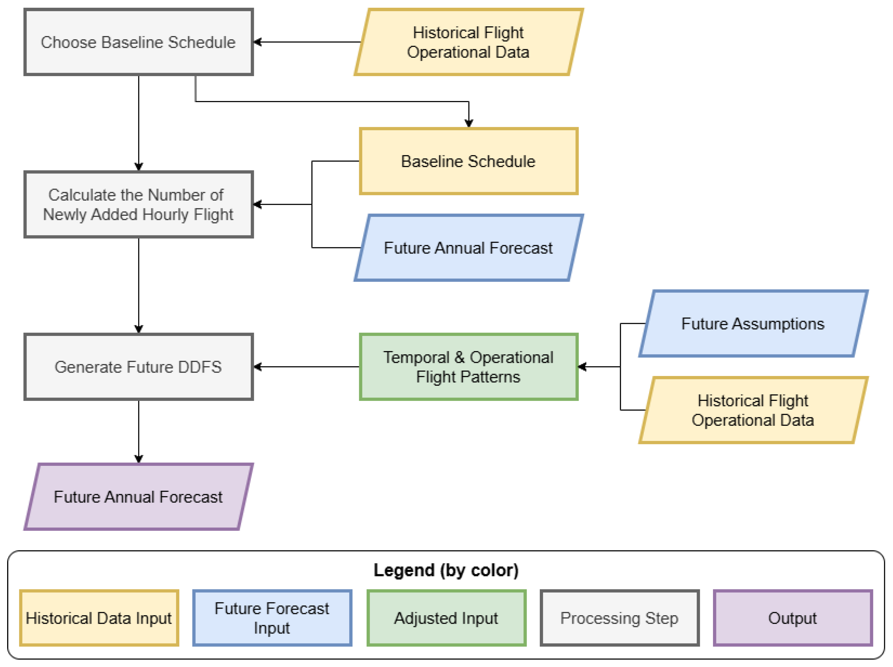
Figure 1 presents the overall framework of the DDFS preparation process. The process begins with the determination of the baseline DDFS from recent flight operations data. The conventional approach to airport planning often utilizes the average day in peak month (ADPM) as the designated design day, although the average day in average month (ADAM) can be employed as an alternative depending on analysis requirements.

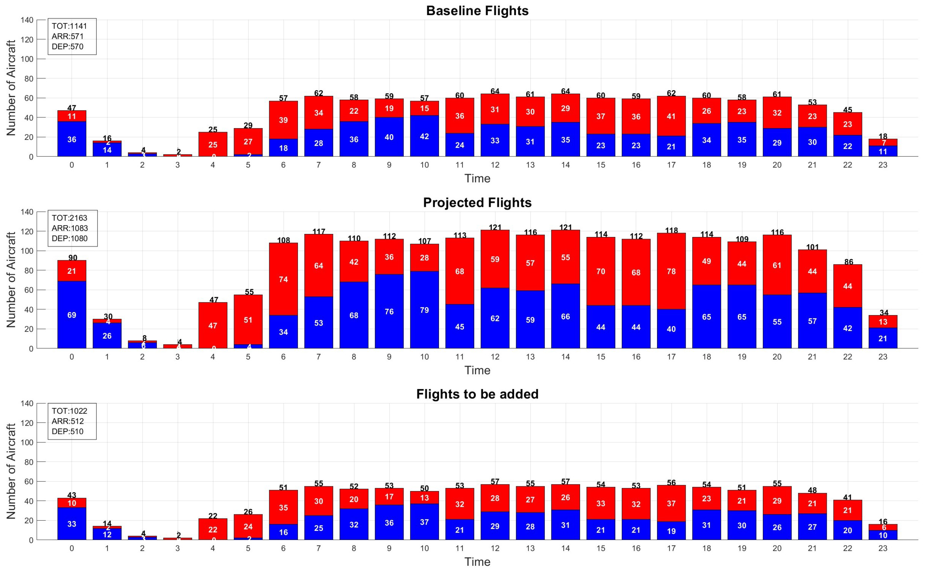
The second step involves determining the number of additional hourly flights by taking the difference between the projected future hourly flights and the baseline DDFS hourly flights. Presented in Figure 2 are the hourly flight operations of the baseline DDFS at Incheon International Airport (ICN), the projected flights for the target year, and the additional hourly flights that will be newly scheduled. In the figure, the additional hourly flights are further divided into two groups, departures (in blue) and arrivals (in red). These additional hourly flights represent the total number of arrival and departure flights to be newly generated in each hour for the target year. The schedule generation procedure assigns detailed operational attributes—such as aircraft type, origin/destination airport—to this predefined set of hourly arrival and departure flights.

In the last and most crucial step, we connect arrival flights with their corresponding departures, considering diverse temporal and operational patterns identified from historical data and reflecting anticipated future trends. This procedure is carried out in an iterative fashion until all additional flights are created. The next section discusses this crucial step in detail.

4. Flight Schedule Generation

A newly generated aircraft is expected to perform three distinct operations in succession: (1) arrival, (2) turnaround, and (3) continued departure. Essentially, the proposed method focuses on identifying and assigning specific attributes to a newly generated aircraft through three operations. Key attributes for an arrival flight include the time of arrival (specifically, in-block time), origin airport, type of operation (whether it is a passenger or cargo flight), aircraft category, and the numbers of both origin/destination and transfer passengers. Similarly, the features related to the subsequent departure include off-block time, destination airport, numbers of origin/destination passengers, and transfer passengers, as well as additional relevant details.

It is important to emphasize that these characteristics are interconnected rather than functioning independently. During 6:00–8:00 a.m., for instance, Incheon International Airport (ICN) experiences a surge of arriving flights from Southeast Asian countries. A majority of these arriving flights are operated by low-cost carriers with two representative aircraft types, B737 and A320. Therefore, the attributes of the newly generated flights are designed to reflect the temporal and operational traits observed at the airport under study.

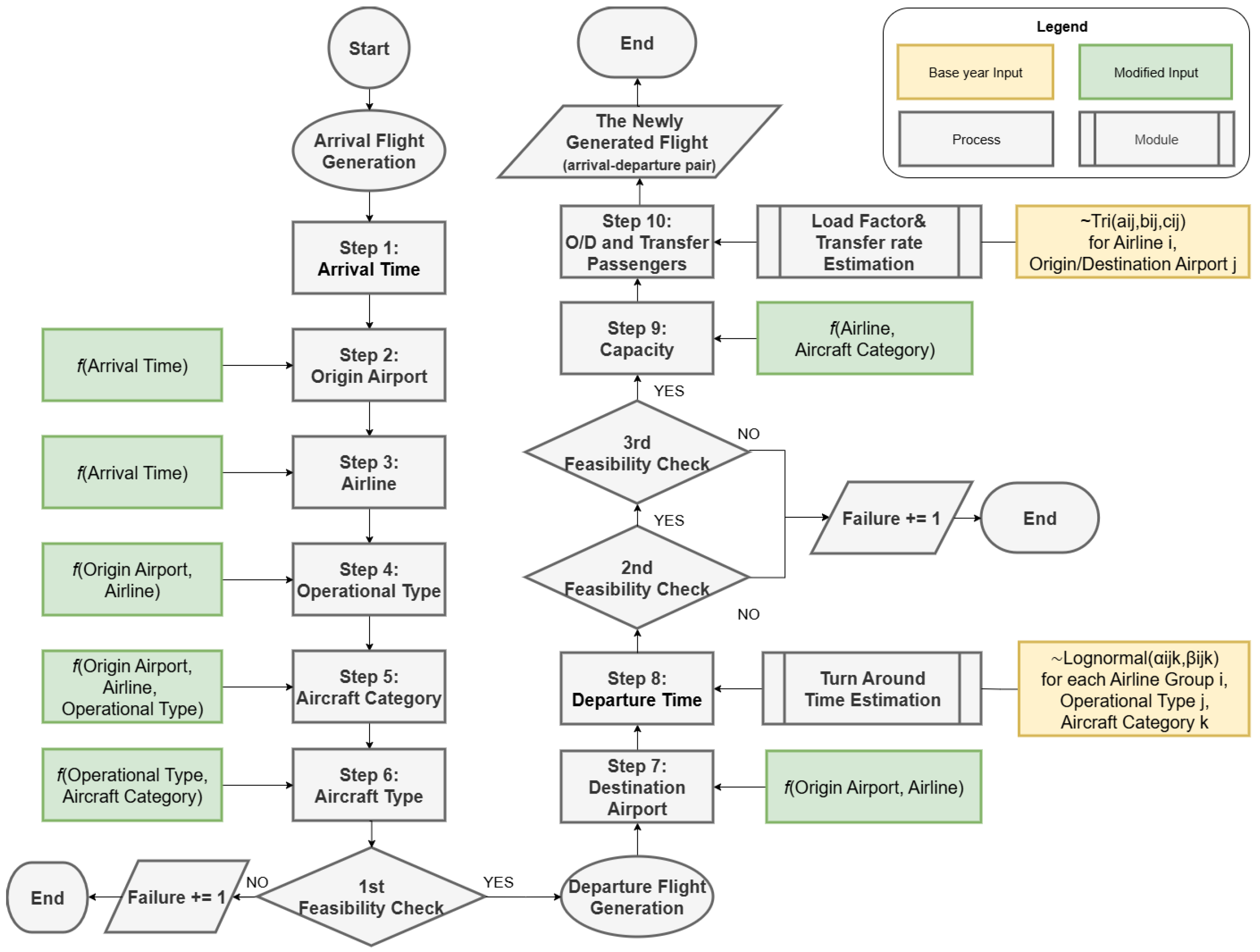
Given the interrelation among attributes, we propose a sequential approach to identify the attributes of newly generated airplanes. Figure 3 presents a comprehensive overview of the steps involved in generating the newly added flight schedule. There are 10 distinct steps, each of which identifies an attribute for a given flight. Steps 1 through 6 focus on determining the characteristics of the arrival flight, while Steps 7 and 8 concentrate on the attributes of the subsequent departure. Steps 9 and 10 determine seating capacity along with the total number of passengers. Over the course of the 10-step attribute generation process, three feasibility tests (represented by rhombuses) are performed to confirm the feasibility of the newly generated flight schedule. When a test is not satisfied, the matching failure counter is incremented by one, and the current generation attempt is terminated.

Given the aggregate number of hourly arrivals and departures that will be newly added, the following outlines the procedure for generating the attributes necessary for the three consecutive operations—arrival, turnaround, and departure—alongside three feasibility tests.

Step 1 (Select an arrival and generate an arrival time, $T^a$):

Step 1-1: Randomly select an arrival from the aggregated number of newly added hourly arrivals and the corresponding hour ($Hr$).

Step 1-2: Given the arrival hour $Hr$ from Step 1-1, randomly choose an arrival time in minutes using a uniform distribution, $M{n}^a\sim U[0,60]$. The candidate arrival time, $T^a$, is the sum of the arrival hour and the minute ($T^a=Hr+M{n}^a$).

Step 2 (Generate origin airport, $O{A}_{t^a}$): Given the arrival time, randomly choose an origin airport for this arrival flight using a probability distribution function (pdf) of origin airport defined as a function of arrival time, derived from past data. When a significant number of origin airports exist, this step can be simplified by grouping airports according to their geographic locations instead of treating each airport independently. This simplification can decrease complexity and reduce the risk of error, as reported by [7]. In our case study, regional groupings practically used by Incheon International Airport Corporation are applied.

Step 3 (Generate airline, $A{L}_{t^a}$): Given the arrival time, randomly choose an airline for this arrival flight using a probability distribution constructed from past data as a function of arrival time.

Step 4 (Generate operational type, $O{T}_{o{a}^i,a{l}^i}$): Randomly select an operation type (i.e., passenger or cargo) for this arrival flight employing a probability distribution defined as a function of airline and origin airport.

Step 5 (Generate aircraft category, $A{C}_{o{a}^i,a{l}^i,o{t}^i}$): Randomly choose an aircraft category for the arrival flight using a probability distribution defined as a function of airline, operation type, and origin airport.

Step 6 (Generate aircraft type, $A{T}_{o{t}^i,a{c}^i}$): Given the operation type and aircraft category, randomly choose an aircraft type for this arrival flight.

Feasibility Test 1 (Verify historical compatibility between aircraft type and origin airport): If the selected aircraft type has been historically operated from the corresponding origin airport, proceed to Step 7. Otherwise, a matching failure is recorded, and the current attempt is terminated.

Step 7 (Generate destination airport, $D{A}_{a{l}^i,o{a}^i}$): Given the airline and origin airport for the arrival flight, randomly choose the destination airport using the pdf of the destination airport defined as a function of airline and origin airport. This step is intended to reflect the underlying tactics employed by airlines in distributing their fleet for connecting flights.

Step 8 (Generate turnaround time $TA{T}_{al{g}^i,o{t}^i,a{c}^i}$ and calculated departure time $T^d$, and connect the arrival with a departure): Turnaround time at an airport usually varies based on airline, operation type (passenger or cargo), and aircraft category. For instance, airlines that use the airport as their main operational base often show a propensity for longer ground times when contrasted with low-cost and foreign carriers. Larger aircraft also require more time to complete turnaround processes. The turnaround time $TA{T}_{al{g}^i,o{t}^i,a{c}^i}$ is randomly decided using a lognormal distribution defined as a function of airline, operation type, and aircraft category. To simplify, airlines may be grouped by factors such as alliance membership, carrier type (legacy versus low-cost), or domestic versus international classification. Once the turnaround time is set, the departure time $T^d$ for the flight is calculated by adding this duration to the arrival time selected in Step 1.

Feasibility Test 2 (Verify connection of the arrival flight with a departure flight): Verify whether there are any remaining hourly departure flights for newly added flights.

Feasibility Test 3 (Verify historical compatibility between aircraft type and the destination airport and establish the arrival-departure connection): Given the aircraft type and the destination airports of the flight, verify whether the aircraft type has been historically operated to that destination airport. Upon positive verification, the connection between this arrival and departure is established. Both the arrival and departure are then eliminated from the list of unscheduled hourly flights. Otherwise, a matching failure is recorded, and the current attempt is terminated.

Step 9 (Identify seat capacity, $CAP{A}_{a{l}^i,a{c}^i}$): Based on the specific airline and aircraft category, determine the average seating capacity associated with the aircraft type utilized by the airline. Average seating capacity can be obtained from past data.

Step 10 (Identify load factor, transfer rate, and the number of O/D and transfer passengers, $LF$, $TF$): Generate random estimates for the load factor and transfer rate of the flight by employing probability distribution functions that characterize the load factor (i.e., the proportion of total passengers to seating capacity) and the transfer rate (i.e., the proportion of transfer passengers) as functions of airline and origin/destination airport pairs. Then, calculate the total number of O/D (origin or destination) and transfer passengers by multiplying these rates by the seat capacity of the aircraft.

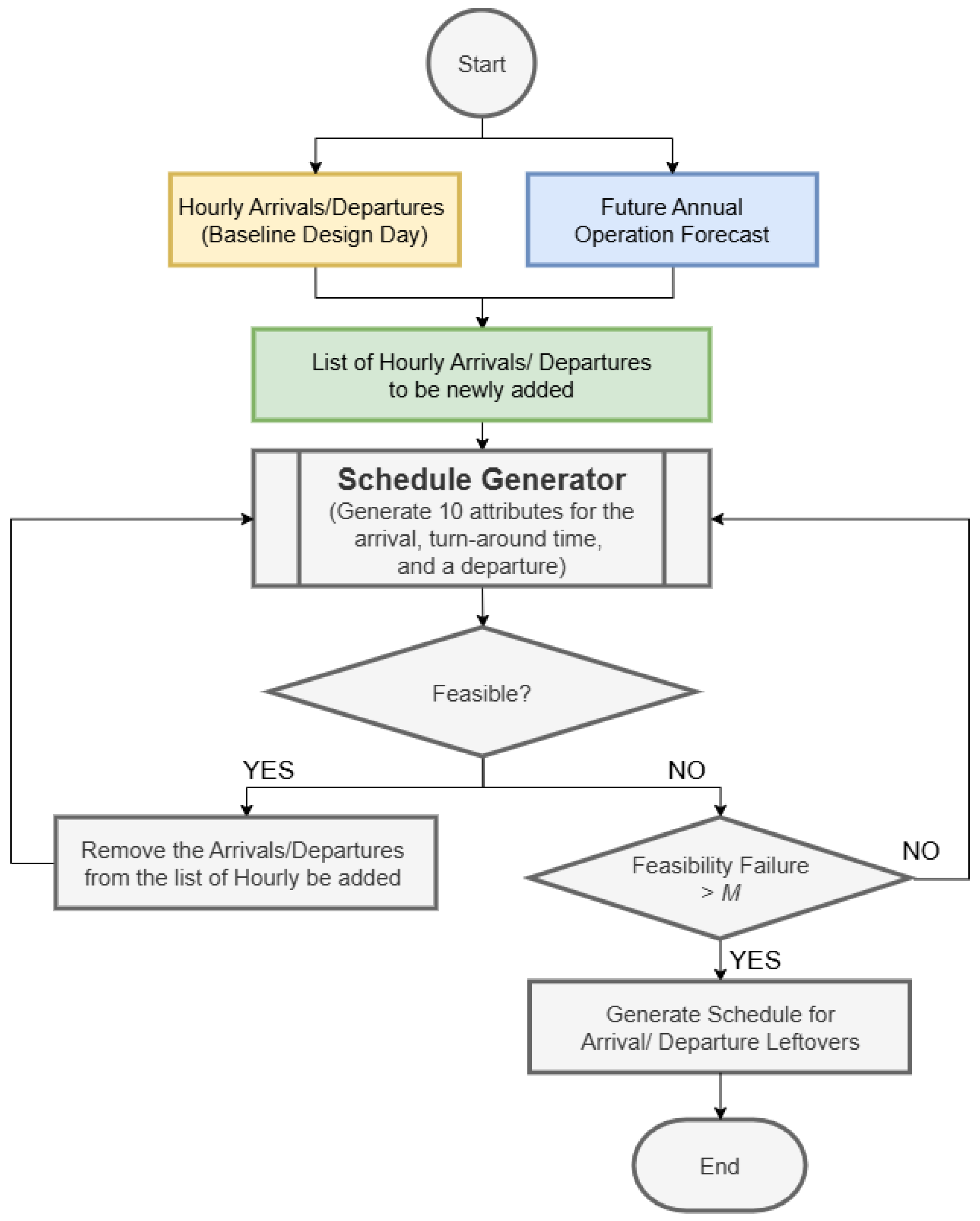
Even after multiple iterations of the whole steps with elimination of arrival–departure paired flights, some arrivals and departures might remain unpaired. This situation occurs mainly because, within the time window considered in the schedule generation process (e.g., a 24-h period), early departures and late arrivals are difficult to pair. These unpaired flights will have only an arrival or departure schedule (instead of a pair) within the time window. Figure 4 illustrates a comprehensive picture of the schedule generation procedure, including the aforementioned 10-step process. As shown in the figure, iteration of the 10-step process stops when the total number of failed feasibility tests reaches a predefined number M. Then we begin generation of schedules for the unpaired flights, applying the 10-step process except for Step 8 (i.e., without determining turnaround time).

Table 1. Randomly generated attributes and associated probability distribution functions.

Notation	Description	Range (or Set)	Probability Distribution Function
$T^a$	Arrival time for an arrival flight	$0\le T^a\le 24$	$T^a=Hr+M{n}^a\sim U[0,60]$
$O{A}_{t^a}$	Origin airport of arrival flight given $t^a$	$OA\in$ airport group set	$f\left(T^a\right) *$
$A{L}_{t^a}$	Airline of arrival flight given $t^a$	$AL\in$ airline set	$f\left(T^a\right) *$
$O{T}_{o{a}^i,a{l}^i}$	Operational type of the arrival flight given $o{a}^i,a{l}^i$	$OT\in \{\mathrm{pax},\mathrm{cargo}\}$	$f(O{A}_{t^a},A{L}_{t^a}) *$
$A{C}_{o{a}^i,a{l}^i,o{t}^i}$	Aircraft category of the arrival flight given $o{a}^i,a{l}^i,o{t}^i$	$AC\in \{A,B,C,D,E,F\}$	$f(A{L}_{t^a},O{A}_{t^a},O{T}_{o{a}^i,a{l}^i}) *$
$A{T}_{o{t}^i,a{c}^i}$	Aircraft type of the arrival flight given $o{t}^i,a{c}^i$	$AT\in$ aircraft type set	$f(O{T}_{o{a}^i,a{l}^i},A{C}_{o{a}^i,a{l}^i,o{t}^i}) *$
$D{A}_{a{l}^i,o{a}^i}$	Destination airport of departure flight given $o{a}^i,a{l}^i$	$DA\in$ airport group set	$f(A{L}_{t^a},O{A}_{t^a}) *$
$TA{T}_{al{g}^i,o{t}^i,a{c}^i}$	Turnaround time of the flight given $al{g}^i,o{t}^i,a{c}^i$	$al{g}^i\in \{\mathrm{National}\mathrm{FSC},\mathrm{LCC},\mathrm{OTHER}\}$	$\sim \mathrm{lognormal}({\alpha }_{al{g}^i,o{t}^i,a{c}^i},{\beta }_{al{g}^i,o{t}^i,a{c}^i})$
$T^d$	Departure time for a departure flight	$0\le T^d\le 24$	–
$CAP{A}_{a{l}^i,a{c}^i}$	Capacity of the flight given $a{l}^i,a{c}^i$	–	$f(A{L}_{t^a},A{C}_{o{a}^i,a{l}^i,o{t}^i}) *$
$L{F}_{a{l}^i,o{a}^i/d{a}^i}$, $T{F}_{a{l}^i,o{a}^i/d{a}^i}$	Load factor and transfer rate of arrival/departure flights given $a{l}^i,o{a}^i/d{a}^i$	$0\le LF,TF\le 1$	$\sim \mathrm{Triangular}\left({\alpha }_{a{l}^i,o{a}^i/d{a}^i}\right)$

Note: * Categorical distribution, where $f\left(x\right)=[x=1]p_1+[x=2]p_2+\cdots +[x=k]p_k$, $\sum p_i=1$. For $k=2$, the distribution reduces to a Bernoulli distribution. $[x=k]=1$ if $x=k$, and 0 otherwise.

presents a summary of the probability distribution functions (pdfs) employed throughout the 10-step procedure. It is important to highlight that historical data collected at the airport serves as the foundation for all pdfs.

It is essential to understand that the randomness incorporated at every step results in a different schedule each time flight schedules are generated. Consequently, the entire process must be repeated several times, after which the best flight schedule is selected to serve as the representative DDFS. In contrast to the feasibility tests in the 10-step process, we define the procedure for choosing the best schedule as a validation process. We discuss the validation process in the case study section.

5. Case Study

This section details the practical application of the proposed method to establish a future DDFS for Incheon International Airport, the primary international airport in South Korea. Recognizing the unprecedented circumstances faced by the aviation industry during the COVID-19 pandemic, which began in mid-2020, we selected 2019 as the base year and designated 2042 as the target year. This means that all probability functions listed in Table 1 are derived from airport data collected in the base year 2019.

In addition, we designate the average day in peak month (ADPM) as the design day, a practice frequently employed in planning airside and terminal facilities. According to International Civil Aviation Organization (ICAO) guidelines, a weekday that demonstrates demand levels similar to the average daily demand during the two months of highest activity is selected to serve as the ADPM [19].

Normally, the airport authority provides results from long-term forecasts for the target year that include annual operations, expected aircraft fleet mix, expected market shares of airlines, and so on.

Table 2. Operational information (base year vs. target year).

		Base Year (2019)	Target Year (2042)
Yearly operations		404,104	764,614
Number of runways		4	5
Runway capacity (operations/h)		107	141
Airline operational share (%)	KE	22.2	22.0
	OZ	15.6	15.2
	Korean LCC	27.6	29.9
	Other	34.6	32.3

and

Table 3. Fleet mix by aircraft category (%).

		Fleet Mix by Aircraft Category (%)
		C	D	E	F
Base year (2019)	Total	53.8	2.7	38.2	5.3
	Pax	58.6	1.2	36.3	3.8
	Cargo	3.5	20.4	65.7	10.4
Target year (2042)	Total	58.9	1.0	38.0	2.1
	Pax	62.7	0.0	36.6	0.7
	Cargo	3.3	16.0	58.2	22.5

shows an example of the information provided by the airport authority for both base and target years.

Applying the annual growth rate from the long-term forecast to the hourly operations of 2019, the initial hourly arrivals and departures in the target year 2042 are obtained, subject to the runway capacity constraint. When the projected hourly demand exceeds this capacity, excess flights are reassigned to nearby high-demand time slots with remaining capacity, reflecting airline scheduling preferences. Figure 2 presents the hourly arrivals and departures for the base year (top), target year (middle), and the increased hourly flights (bottom), which are subsequently detailed using the proposed methodology to generate and allocate the necessary attributes.

By generating random numbers from the probability distribution functions listed in Table 1, each attribute involved in DDFS development is established in the same sequence as outlined in Figure 3. For clarity, we present a few steps as representative examples. Step 2 in Figure 3 determines the origin airport for a given arriving flight. Treated as a discrete random variable, the origin airport of an arriving flight is assumed to follow a distribution $f\left(T^a\right)$, which means the origin airport is randomly distributed according to TOD (see Table 1).

Table 4. Distribution of origin airport regions for arriving flights by time of day.

TOD	Asia	East–South Asia	West–South Asia	China	…	North America	Oceania	Russia	South America
0	14.9%	17.6%	0.1%	21.8%		15.4%	0.7%	7.4%	0.0%
1	2.5%	7.6%	0.1%	37.5%		19.5%	0.1%	1.5%	0.1%
2	2.0%	4.9%	0.0%	55.5%		17.8%	0.3%	3.8%	0.0%
3	24.4%	2.4%	0.1%	3.7%		59.6%	0.1%	1.2%	0.1%
4	5.5%	43.1%	0.0%	9.8%		25.4%	2.9%	2.4%	0.0%
5	16.3%	51.5%	1.6%	11.8%		9.2%	4.9%	1.9%	0.0%
6	11.6%	70.7%	2.4%	2.7%		1.5%	8.7%	0.3%	1.6%
					…
10	11.2%	31.8%	0.8%	29.0%		5.0%	0.9%	3.8%	0.0%
					…
21	10.4%	27.1%	0.0%	18.9%		2.9%	3.3%	4.8%	0.6%
22	10.0%	30.6%	0.0%	15.9%		1.4%	0.8%	4.7%	0.1%
23	12.0%	21.6%	0.1%	12.5%		7.3%	1.0%	10.6%	0.0%

illustrates probability distributions of origin airports by hour (i.e., TOD), reflecting historical distribution patterns. For a high level of granularity, all origin airports are grouped into 13 regions of the world.

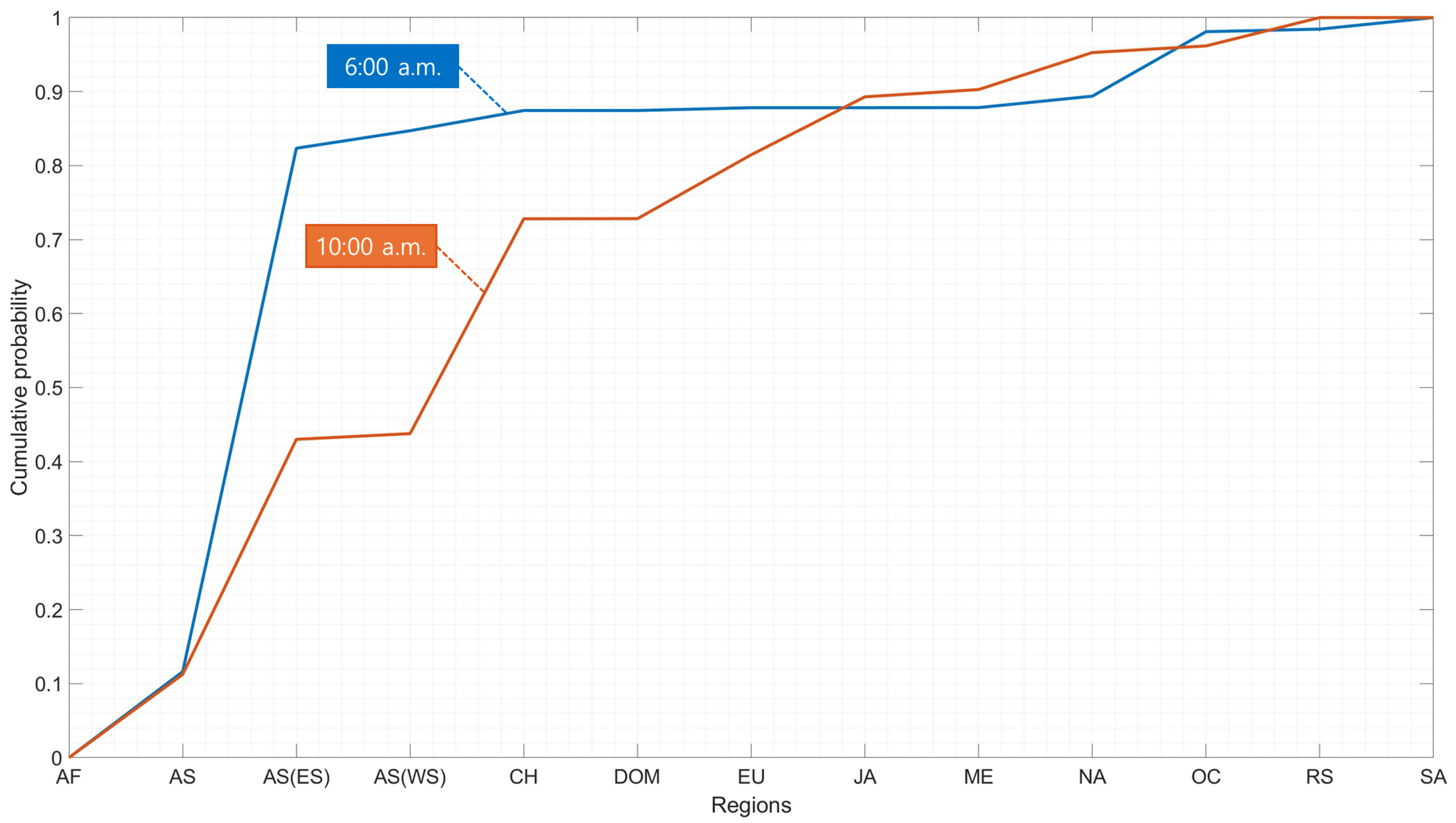
The distribution patterns of origin regions are clearly distinguished over time. For instance, about 70% of arrival flights landing between 6:00 and 7:00 a.m. are from East-South Asia, including Vietnam and Thailand. In contrast, during 10:00–11:00 a.m., routes for arriving flights are more diversified, including China (CH), Europe (EU), and Japan (JA). Figure 5 compares these cumulative distributions over 13 regions, which clearly demonstrates that routes for arrival flights vary according to TOD.

If the proportion of routes is anticipated to change in the target year, the distribution can be modified accordingly. For example, if demand from a specific market is expected to increase substantially in the future, the distribution can be adjusted to reflect this change. The projected future-to-current ratio is applied to the historical distribution, and the resulting adjusted distribution is then used to generate the newly added flights. In this way, anticipated changes in future traffic composition can be reflected in the generated DDFS.

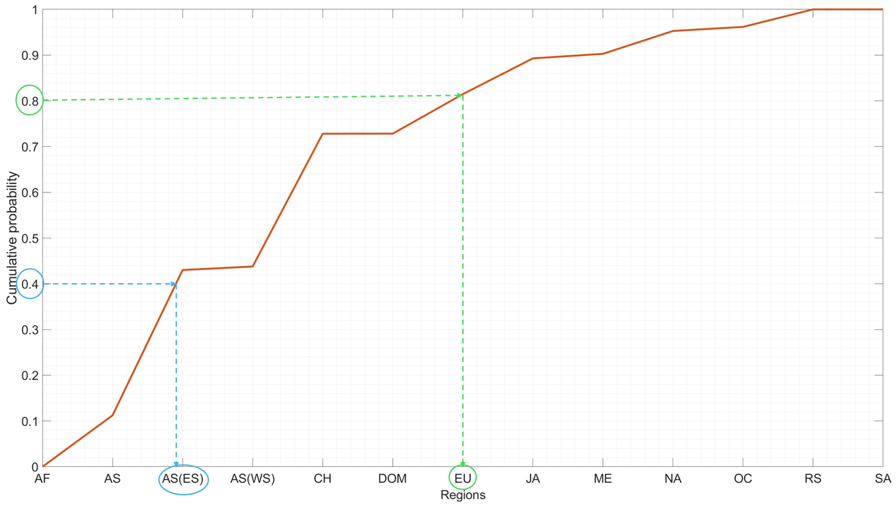
After constructing the cumulative probability distributions, the next step involves randomly determining the origin region for a flight arriving at a specific time of day. This process includes generating a random number between 0 and 1, comparing it to the cumulative probabilities associated with the arrival time of the flight, and designating the origin region whose cumulative probability contains the random number. For instance, if the specified arrival time is 10:00 a.m., Figure 6 illustrates the cumulative probability distribution for that time. If a random number of 0.8 is drawn, Europe is chosen as the origin region (green dotted line). Conversely, if the number is 0.4, Southeast Asia is selected (blue dotted line). Each attribute of an arriving flight, as described in Steps 3 through 6, is determined in a similar way. This approach allows us to capture established operational patterns while also adding diversity through random sampling. Steps 3 through 6, as shown in Table 1, identify the additional attributes needed for an arriving flight.

Here, it is important to recognize that these attributes are independently generated at each step, and thus interdependencies among attributes are not fully captured. To verify such interdependencies, the first feasibility test in Figure 3 is carried out. In this verification step, we check the flight distance of the arriving flight against the flight range of the aircraft type. If the flight distance is within the range of the selected aircraft type, the arrival flight schedule is finalized; otherwise, the procedure returns to the first step, and the sampling process is repeated until a feasible combination is obtained.

Once the attributes for each arrival flight are assigned, the attributes for the continued departure are determined. As shown in Figure 3, there are two key attributes to be decided: (1) the region of the destination airport, assumed to be a function of airline and origin region of the previous arrival flight, $f(O{A}^i,A{L}^i)$; and (2) the scheduled departure time derived from turnaround time. Statistical information pertaining to the interconnections between airlines, originating regions, and terminating regions for continuing flights is derived from historical records.

Table 5. Distribution of origin and destination airport regions for continued flights (Korean Air).

	Destination	Asia	East–South Asia	West–South Asia	China		North America	Oceania	Russia	South America
Origin
Africa		0.0%	50.0%	0.0%	16.7%		0.0%	0.0%	16.7%	0.0%
Asia		5.8%	22.4%	1.3%	18.8%		11.5%	6.3%	1.4%	0.4%
East–South Asia		5.8%	40.2%	1.2%	21.5%		6.5%	3.7%	2.2%	0.5%
West–South Asia		8.0%	14.7%	0.6%	24.3%		0.6%	1.1%	8.0%	0.0%
China		6.7%	27.0%	2.0%	19.7%		4.0%	6.1%	2.5%	0.4%
Domestic		6.9%	7.2%	0.1%	24.4%		0.0%	2.1%	0.6%	0.0%
EU		6.9%	9.8%	2.3%	6.0%	…	30.1%	5.7%	1.3%	2.4%
Japan		4.4%	11.0%	1.2%	25.1%		9.4%	2.0%	3.1%	0.1%
Middle East		13.5%	21.0%	13.5%	11.3%		1.3%	4.9%	1.6%	0.0%
North America		7.6%	19.0%	0.0%	5.3%		29.9%	7.2%	0.2%	0.9%
Oceania		8.4%	30.5%	3.6%	10.1%		13.7%	13.9%	0.7%	0.0%
Russia		7.7%	19.9%	5.4%	6.9%		5.9%	12.8%	9.0%	0.0%
South America		14.1%	15.6%	0.4%	19.1%		12.9%	0.0%	0.0%	4.3%

illustrates a representative distribution of destination regions for continued flights operated by Korean Air, given an origin region.

Random selection of the destination airport region for a continued departure is performed in Step 7, utilizing the probability distribution prepared for each airline. Once the destination region for the continued departure is determined, the second feasibility test is conducted to verify that the destination is within the flight range of the given aircraft type.

Another key attribute of a departure flight is the scheduled departure time, which is determined by adding the turnaround time to the scheduled arrival time. Turnaround time is defined as the interval between an aircraft’s arrival at the gate and its subsequent departure and is affected by aircraft size and airline operational policies [7]. In addition to these two elements, we also consider the operation category (passenger or freight), given differences in pre-operational processes. Collectively, turnaround time is presumed to be a function of airline, aircraft size, and operation type. Using historical information, we model a lognormal distribution for each combination of airline, aircraft type, and operation type.

The turnaround time for a given departure, factoring in airline, aircraft type, and operation type, is randomly generated from the fitted distribution. With the calculated departure time, the second feasibility test is conducted to ensure that there are at least hourly departure flights for the newly added flights. This test verifies that the number of flight operations within a time period remains below the established threshold. The final feasibility test then verifies the historical compatibility between the aircraft type and the destination airport and, if satisfied, establishes the corresponding arrival–departure connection. Upon successful completion of the feasibility assessment, the attributes designated for the departure flight are finalized.

The last step is to determine the seat capacity for the aircraft and the number of passengers for its arrival and departure flights. Seating capacity for a particular aircraft category is determined by employing the average seat capacity derived from historical data.

The number of passengers is divided into O/D passengers and transfer passengers, as their different facility-use behaviors are relevant to terminal analysis. These counts are calculated by applying the load factor and transfer rate to aircraft capacity. To generate passenger numbers stochastically, a triangular distribution is utilized for both load factor and transfer rate estimation. We define the load factor and transfer rate as functions of the airline and the origin/destination airports. For each airline and airport, mean, minimum, and maximum values for the month containing the design day are obtained from historical data and adopted for fitting the triangular distributions.

The steps above generate one line of the schedule. The steps are repeated until all newly added flights are generated. However, because arrivals are generated prior to departures, some early departures and late arrivals fail to be paired and remain as leftovers. We therefore repeat the process for a preset number of iterations and then generate leftover arrivals and departures as independent flights. Once all leftover flights are generated, the future design-day schedule is finalized as a complete set.

5.1. Computational Results

Iteration of the 10 sequential steps continues until all newly added flights (as defined in Figure 2) have been successfully generated. Upon completion of Steps 1 through 10, a new flight schedule is produced.

Because each flight schedule generated through these steps includes randomly assigned attributes based on different probability distribution functions (summarized in Table 1), each full DDFS set is distinct. To account for this variability, multiple DDFS sets are generated, and then the set that best matches the target-year forecasts—specifically, (1) peak-hour flight volume on the design day and (2) fleet mix—is selected.

In the case study, a total of 60 DDFS sets are generated. To assess the overall reliability of the generated schedules, the mean error between each schedule and the corresponding future forecasts is computed. Descriptive statistics for the two indicators are reported in

Table 6. Overall statistics of 60 DDFS schedules.

	Peak Hour Operation [Ops/Hr]	MAE of Fleet Mix [%]
Mean	130	1.47
Median	130	1.48
Mode	130	1.23
Std. Deviation	3.59	0.32
Min value	124	0.63
Max value	142	2.16

.

Low standard deviations (Std.Deviation in Table 6) for both indicators indicate limited variability among the generated schedules, thereby demonstrating the stability of the proposed method. Having established stability, the reliability of the generated schedules is evaluated by comparing the peak-hour operations and fleet mix derived from the 60 DDFS sets with the future forecast. The peak-hour forecast is independently obtained by applying the ADPM–PH factor to the annual forecast, yielding 130 operations per hour for the target year. As shown in Table 6, the mean, median, and mode of peak-hour operations across the 60 DDFS sets closely match the future value. In addition, the results of the mean absolute error (MAE) analysis for the fleet mix show that the mean, median, and mode of the MAE remain within approximately 1%. The MAE of the fleet mix is calculated by comparing for each aircraft category (C, D, E, and F), the proportion specified in the future forecast with the corresponding proportion in each individual DDFS. These results collectively demonstrate an agreement between the generated DDFSs and the future forecast.

Then, the DDFS set that best matches the future forecasts is selected as the final (best) DDFS.

Table 7. Fitness of resulting DDFS relative to future forecast.

	Fleet Mix (%)				Peak-Hour Operations
	C	D	E	F
Future forecast	58.9	1.0	38.0	2.1	130
Best DDFS	56.8	1.5	39.1	2.6	130

compares its two indicators with the corresponding forecast values, and

Table 8. Excerpt of the selected DDFS.

Airline	Pax/Cargo	Aircraft Cat.	Aircraft Type	Arrival				Departure
				Schedule Time	Origin (Region)	O/D Pax	Transfer Pax	Schedule Time	Dest. (Region)	O/D Pax	Transfer Pax
OZ	PAX	E	330	00:40	EU	185	28	06:31	AS(ES)	180	34
KE	CARGO	E	777	14:38	CH			20:30	AS(ES)
KE	PAX	E	777	17:34	NA	157	55	18:57	OC	162	50
OZ	PAX	E	350	04:58	NA	182	75	06:55	AS(ES)	183	35
OZ	PAX	C	320	18:38	JA	78	26	20:57	JA	80	26
KE	PAX	E	747	05:55	AS(ES)	234	56	17:18	AS(ES)	229	54
OZ	PAX	E	777	04:11	AS(ES)	190	35	17:58	AS(ES)	176	33
LJ	PAX	E	737	07:50	AS(ES)	148	7	09:40	AS	150	8
KE	PAX	E	330	06:16	AS(ES)	145	34	07:39	CH	150	30
7C	PAX	E	737	13:17	JA	157	7	14:03	JA	143	6

presents an excerpt.

5.2. Validation

For the chosen DDFS, further validation is performed to ensure conformance with both future forecasts and historical patterns.

To evaluate how well the resulting DDFS captures future changes, the proportions of airline operations from the selected DDFS set are compared with future forecasts (

Table 9. Airline operation ratio error between DDFS and future forecast.

		Future Forecast (=A)	DDFS (=B)	Error (B–A)
		(1)	(2)	(3)
Airline Operation Ratio (%)	KE	22.6	23.5	$0.9\%p$
	OZ	15.2	17.8	$2.6\%p$
	Korean LCC	29.9	31.3	$1.5\%p$
	Other	32.3	27.4	$-4.9\%p$

). As shown in the table, the airline shares derived from the DDFS align closely with the forecasts, remaining within a $\pm 5$% percentage-point error band.

In addition to capturing future changes, alignment with historical operational patterns is also evaluated using two factors: (1) the distribution of connection route pairs (i.e., origin region of inbound flight and destination region of outbound flight) for a given aircraft, and (2) turnaround time by aircraft type.

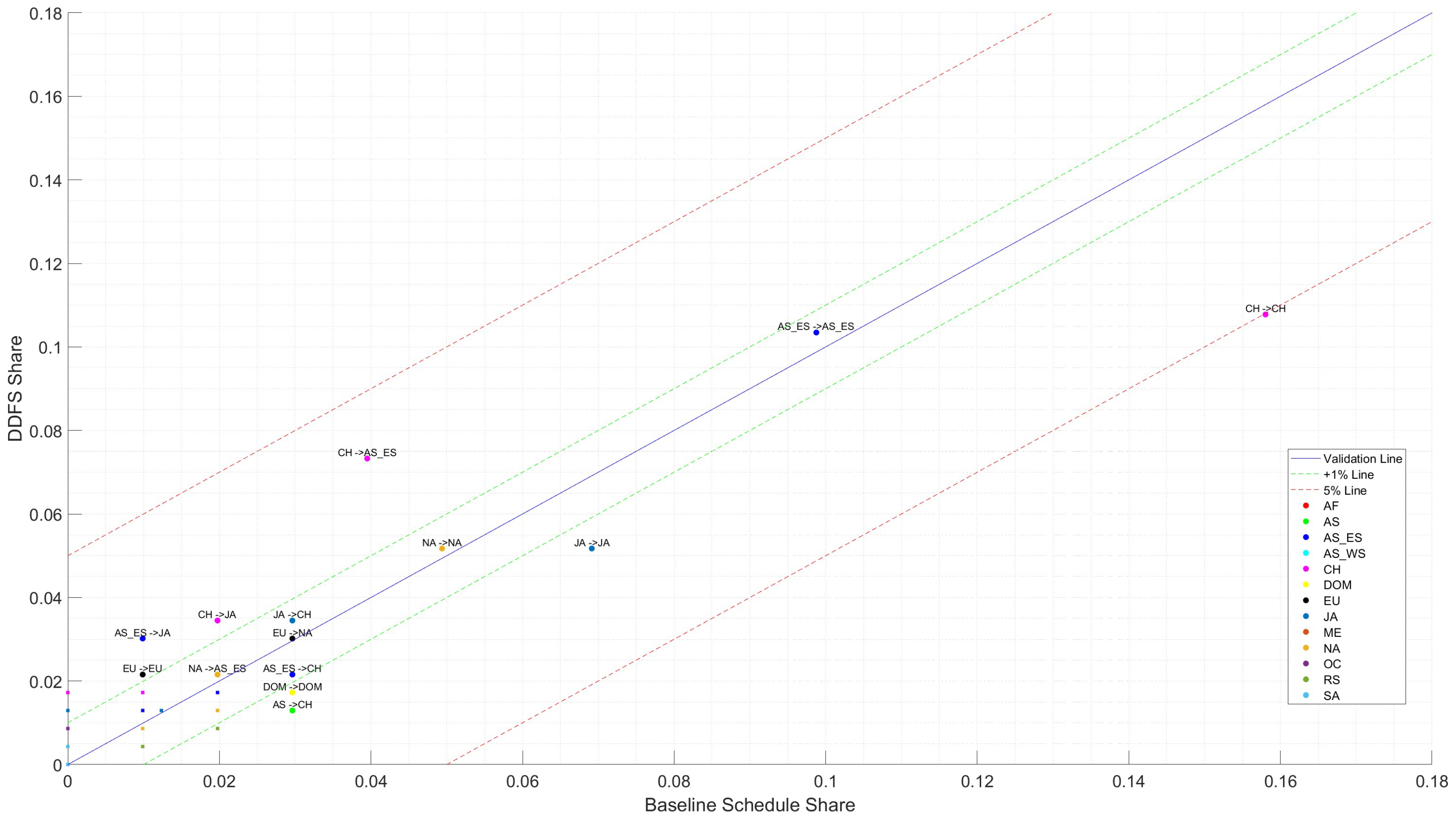
As an example, connecting route-pair patterns of Figure 7 illustrate the validation of connecting route-pair patterns for Korean Air flights by comparing observed shares from the baseline schedule (x-axis) with DDFS-derived shares (y-axis). The 45° line indicates perfect agreement, and the dashed green lines denote the ±1 percentage-point error bands, and dashed red lines denote ±5 percentage-point error bands.

For instance, the North America → North America (NA → NA in the plot) route pair illustrates the comparison, with observed and DDFS-derived shares of 4.9% and 5.2%, respectively. As shown in the figure, all points lie within the ±5 percentage-point error bands, and most fall within the ±1 percentage-point bands. The overall fit is high, with an MAE of 0.002 (0.2%). Overall, these results suggest that the DDFS effectively captures historical patterns.

The distributional characteristics of turnaround time (TAT) are also examined to assess how well the assumed probabilistic models reproduce historical operational patterns. To quantitatively evaluate the agreement between the empirical and fitted TAT distributions, the Kolmogorov–Smirnov (KS) statistic was computed for each airline–operation–aircraft segment. The resulting KS statistics ranged from 0.046 to 0.301 across segments. Lower values were generally observed for relatively homogeneous airline groups, whereas larger deviations appeared in more heterogeneous categories (e.g., “Other” airlines), reflecting differences in operational practices and variability in turnaround behavior. Overall, the results indicate that the fitted distributions capture the empirical TAT patterns with reasonable agreement across segments.

Turnaround time is further evaluated by comparing average values by aircraft category between the baseline design day and the DDFS (

Table 10. Validation result on turnaround time.

Average Turnaround Time
	ADPM Design Day (=A)	DDFS (=B)	Error (B/A)
C	154.9	140.6	0.90
D	151.4	197.0	1.30
E	244.6	259.5	1.10
F	331.3	205.0	0.60

). Errors remain within ±5 percentage points, indicating close agreement with observed operations. The results demonstrate that the adopted models reproduce key operational characteristics with sufficient accuracy for realistic DDFS generation.

6. Conclusions and Recommendations

Due to the accessibility of digital data procured via recently implemented airport information systems, simulation analysis is recognized as a more powerful and practical way for comprehensive planning, design, and operation of airports. For the purpose of simulation analysis, the design day flight schedule (DDFS) constitutes a crucial prerequisite. Recognizing the importance of DDFS in simulation analysis, leading organizations such as IATA and ACRP have provided overall guidelines for DDFS considerations and a comprehensive process; however, detailed methodological documentation is scarce. Motivated by the practical gap, this paper presents a data-driven 10-step procedure for the generation of DDFS. The main idea underlying the procedure is described in the following manner: (1) The DDFS for the target year is derived through the superimposition of the new flight schedule onto the base-year flight schedule. (2) The attributes necessary for defining a flight schedule encompass the carrier, flight classification (passenger or freight), aircraft type, scheduled time, origin (or destination) airport, the number of passengers, etc. (3) For an individual aircraft, the schedules for both its arrival and departure are produced by means of consecutively identifying the pertinent attributes. (4) The attributes are identified via a probabilistic approach utilizing probability distribution functions that are derived from the historical data collected at the airport. (5) The stochastic nature inherent in the entire process ensures that the generated DDFSs are mutually distinct. To accommodate the inherent variability of DDFS, multiple DDFS instances are generated, and the most advantageous one is subsequently chosen based on predefined criteria.

A case study was conducted in which 60 DDFS sets were generated for Incheon International Airport for the year 2042. The generated schedules exhibit limited variability across trials, suggesting that the proposed methodology produces stable and consistent outputs. The best-performing set is selected based on its agreement with the target-year forecasts for fleet mix and peak-hour flight volume on the design day. The selected DDFS is further validated against future forecasts and historical patterns across multiple operational dimensions, with most discrepancies within a 5% error range. Overall, the approach demonstrated through this case study may serve as a practical framework for developing functional DDFS.

Potential improvements for the suggested method include:

(1) Ten-step procedure can be further refined. For instance, in the case study, the load factor and transfer rate are both determined according to the aircraft category. However, the factor and rate can be established additionally, considering O-D airport pairs and time of day.

(2) Sensitivity or scenario-based analyses can be conducted to examine how variations in key planning assumptions influence the generated DDFS. For instance, alternative fleet-mix or operational-profile scenarios reflecting potential airline strategy shifts or fleet modernization trends may be explored.

(3) While distribution parameters were empirically estimated, formal statistical goodness-of-fit tests were not conducted, which represents a methodological limitation. It is recommended that statistical tests be performed whenever a probability distribution function is used in order to verify the function’s significance.

(4) The within-hour arrival time generation may be further refined. While a uniform distribution over 0–60 min was adopted in this study, future research may incorporate structured within-hour patterns reflecting banking/wave structures, airline push patterns, or demand peaking behavior.

(5) The determination of the most appropriate DDFS can be performed with specificity (micro-level) rather than generality (macro-level). The hourly distribution of origin-destination airport traffic over 24 h, for instance, can be an additional evaluative measure for the choice of the DDFS. Similarly, if the projected fleet mix is available at the airline level, the DDFS can be evaluated by leveraging the specific fleet mix of each airline. In addition, the selection process can be extended to incorporate more detailed temporal characteristics, such as short-interval congestion patterns observed over 15-min windows, to better reflect conditions relevant to detailed simulation.

(6) Although the framework is demonstrated using a large, slot-coordinated hub airport, its application to airports with different operational characteristics—such as smaller hubs or domestic-focused airports—can be explored by appropriately redefining the input parameters and distributions, which is left for future research.

(7) In the same vein, the selection criteria for a representative DDFS are application-dependent. While fleet mix and peak-hour operations were emphasized in this study, alternative uses may require different criteria. The proposed methodology, therefore, provides a flexible framework that can be adapted to various planning and simulation objectives.

Despite these limitations, this study contributes by explicitly formulating a reproducible, data-driven process for developing future Design Day Flight Schedules based on empirical airport data. By documenting how long-term demand forecasts are translated into flight-level schedules through a structured procedure, the proposed framework improves the reproducibility of DDFS construction in simulation-based airport studies. In this regard, it can serve as a practical reference for researchers and practitioners who require well-documented and consistent schedule inputs.