Figure 1.
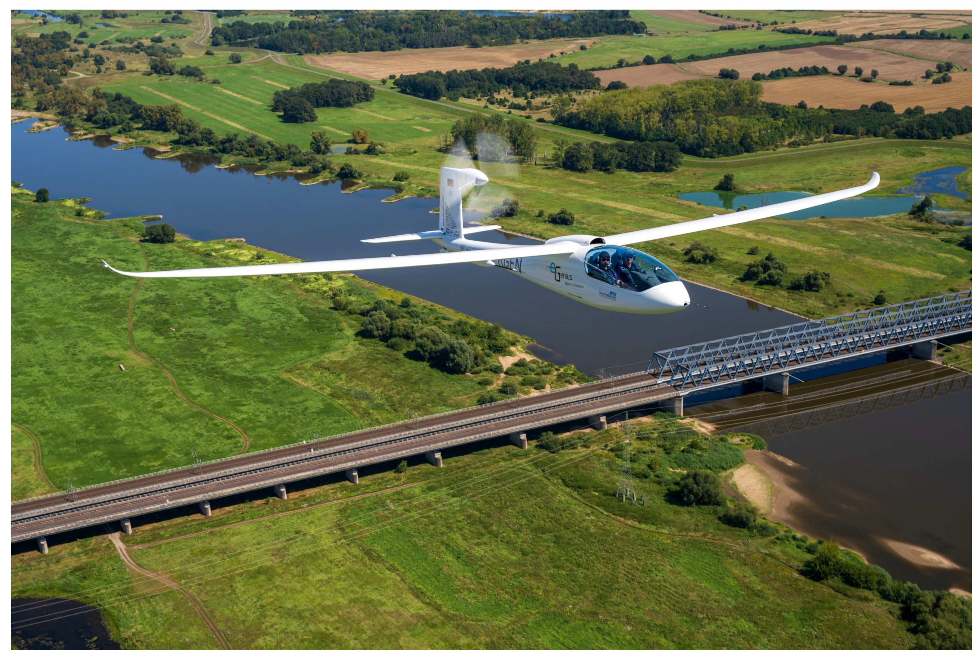
e-Genius in its fully battery-electric configuration. Photographed by Tobias Barth.
Figure 1.
e-Genius in its fully battery-electric configuration. Photographed by Tobias Barth.
Figure 2.
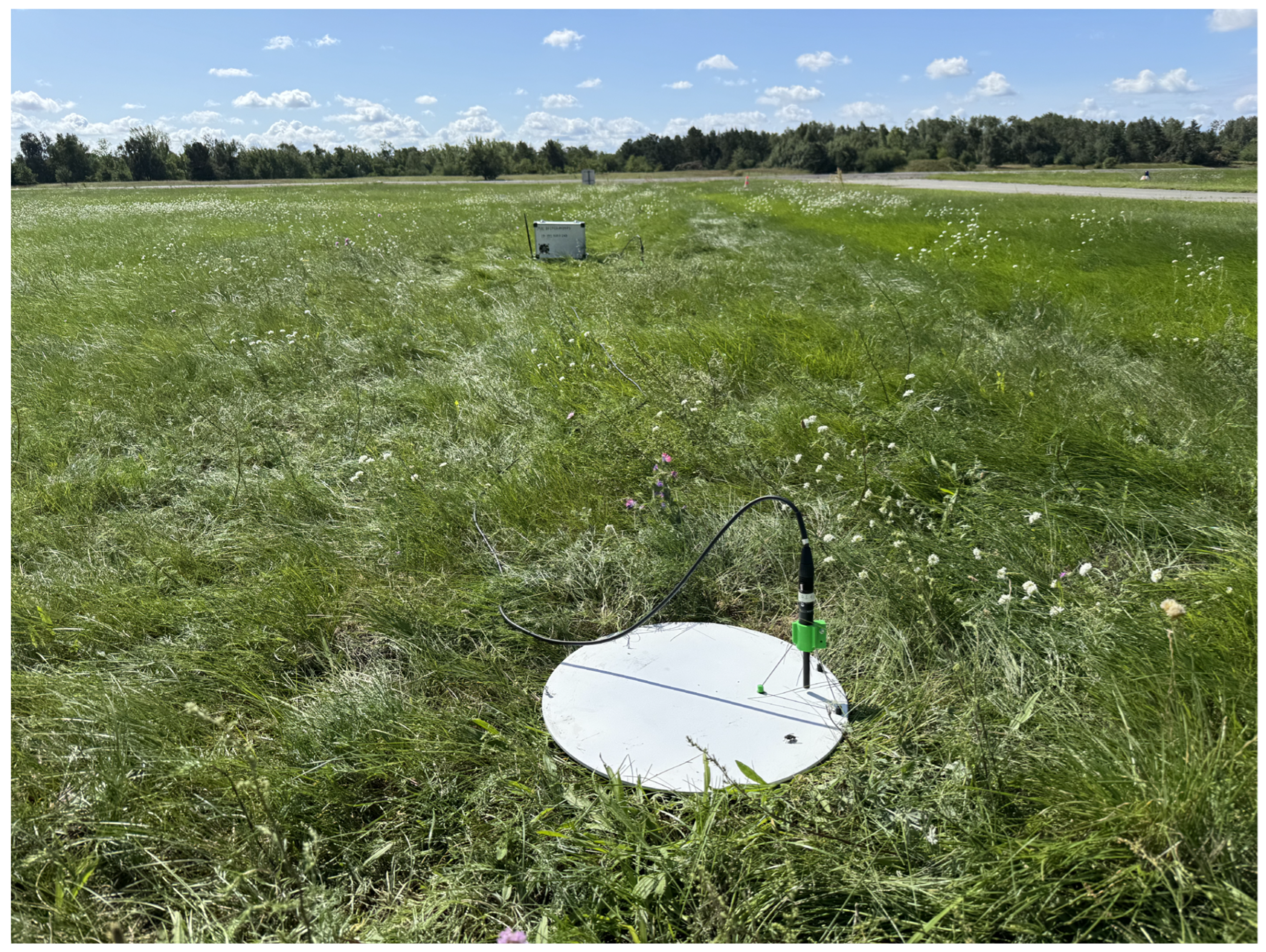
Noise measurement setup: microphone mounted upside down on a ground plate. In the background, one of the measurement boxes can be seen.
Figure 2.
Noise measurement setup: microphone mounted upside down on a ground plate. In the background, one of the measurement boxes can be seen.
Figure 3.
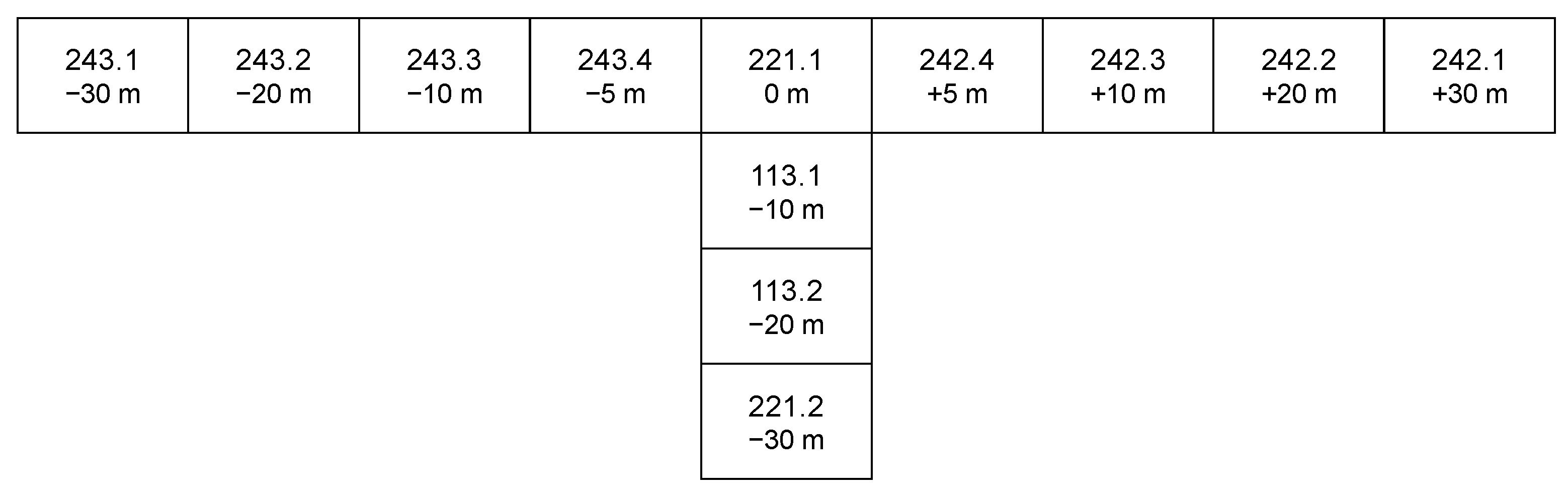
Noise measurement setup: microphone arrangement (box.channel), including relative distances to the center microphone.
Figure 3.
Noise measurement setup: microphone arrangement (box.channel), including relative distances to the center microphone.
Figure 4.
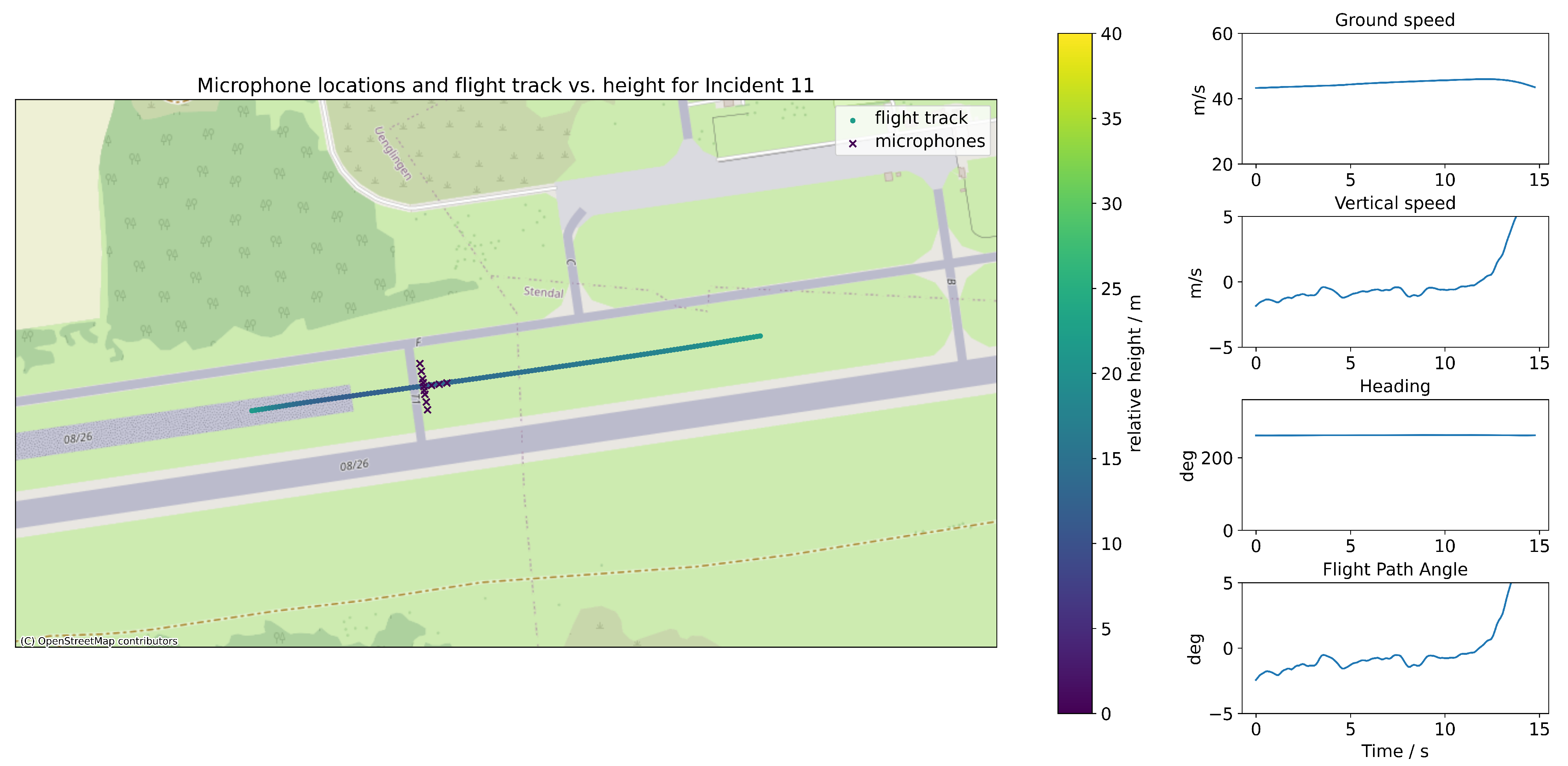
Example ground track, derived from incident 11, recording 1. Microphone positions are marked as x, and the height above the center microphone is represented by the color of the track. At the end of the sequence, roughly at time 12.5 s, the power is increased and a climb is initiated, as can be seen in the vertical speed and flight path angle.
Figure 4.
Example ground track, derived from incident 11, recording 1. Microphone positions are marked as x, and the height above the center microphone is represented by the color of the track. At the end of the sequence, roughly at time 12.5 s, the power is increased and a climb is initiated, as can be seen in the vertical speed and flight path angle.
Figure 5.
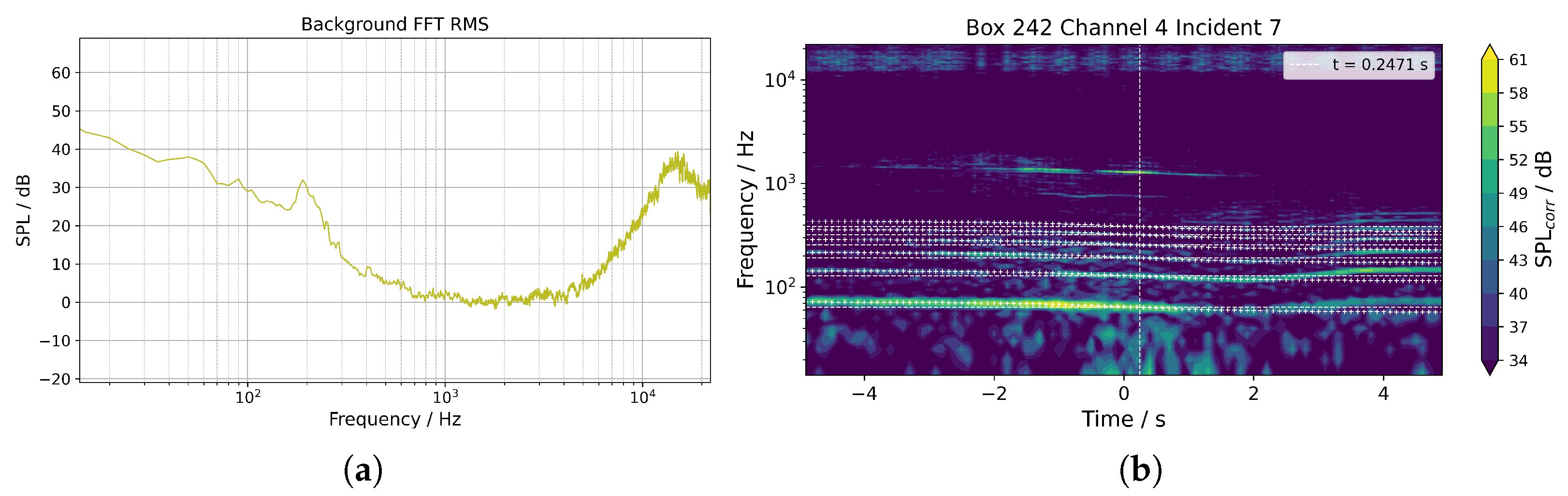
Influence of crickets on the noise measurement. (a) RMS of all FFTs performed for one background noise excerpt. There is a very distinct increase in SPL beginning roughly at 4000 Hz. (b) During the overflight, the chirping of the cricket is still seen in the FFT graph at high frequencies after correcting for the background signal, where SPLcorr is the background-corrected SPL. Furthermore, aircraft noise features are partially removed.
Figure 5.
Influence of crickets on the noise measurement. (a) RMS of all FFTs performed for one background noise excerpt. There is a very distinct increase in SPL beginning roughly at 4000 Hz. (b) During the overflight, the chirping of the cricket is still seen in the FFT graph at high frequencies after correcting for the background signal, where SPLcorr is the background-corrected SPL. Furthermore, aircraft noise features are partially removed.
Figure 6.
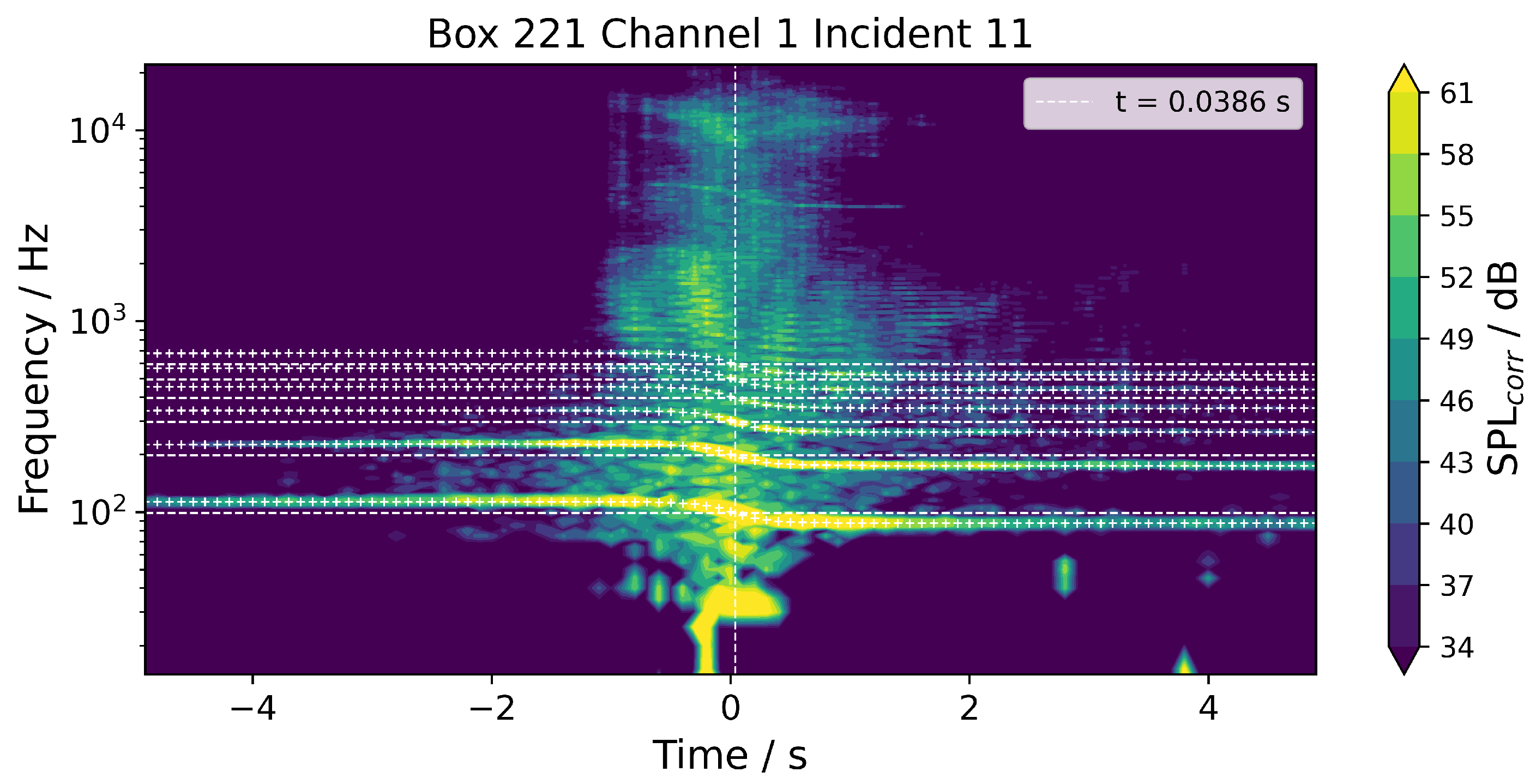
FFT over time for the center microphone (221.1) for the incident 11 of the first flight. Time 0 s is exactly when the aircraft overflies the microphone. Taking into account the propagation time (speed of sound, t = 0.0386 s), the vertical dashed line marks the overflight time as recorded by the microphone. The horizontal dashed lines mark the ideal first six BPFs without a Doppler shift. Furthermore, the + signs mark the calculated Doppler-shifted first six BPFs based on the relative velocity from the GPS. SPLcorr is the background-corrected SPL.
Figure 6.
FFT over time for the center microphone (221.1) for the incident 11 of the first flight. Time 0 s is exactly when the aircraft overflies the microphone. Taking into account the propagation time (speed of sound, t = 0.0386 s), the vertical dashed line marks the overflight time as recorded by the microphone. The horizontal dashed lines mark the ideal first six BPFs without a Doppler shift. Furthermore, the + signs mark the calculated Doppler-shifted first six BPFs based on the relative velocity from the GPS. SPLcorr is the background-corrected SPL.
Figure 7.
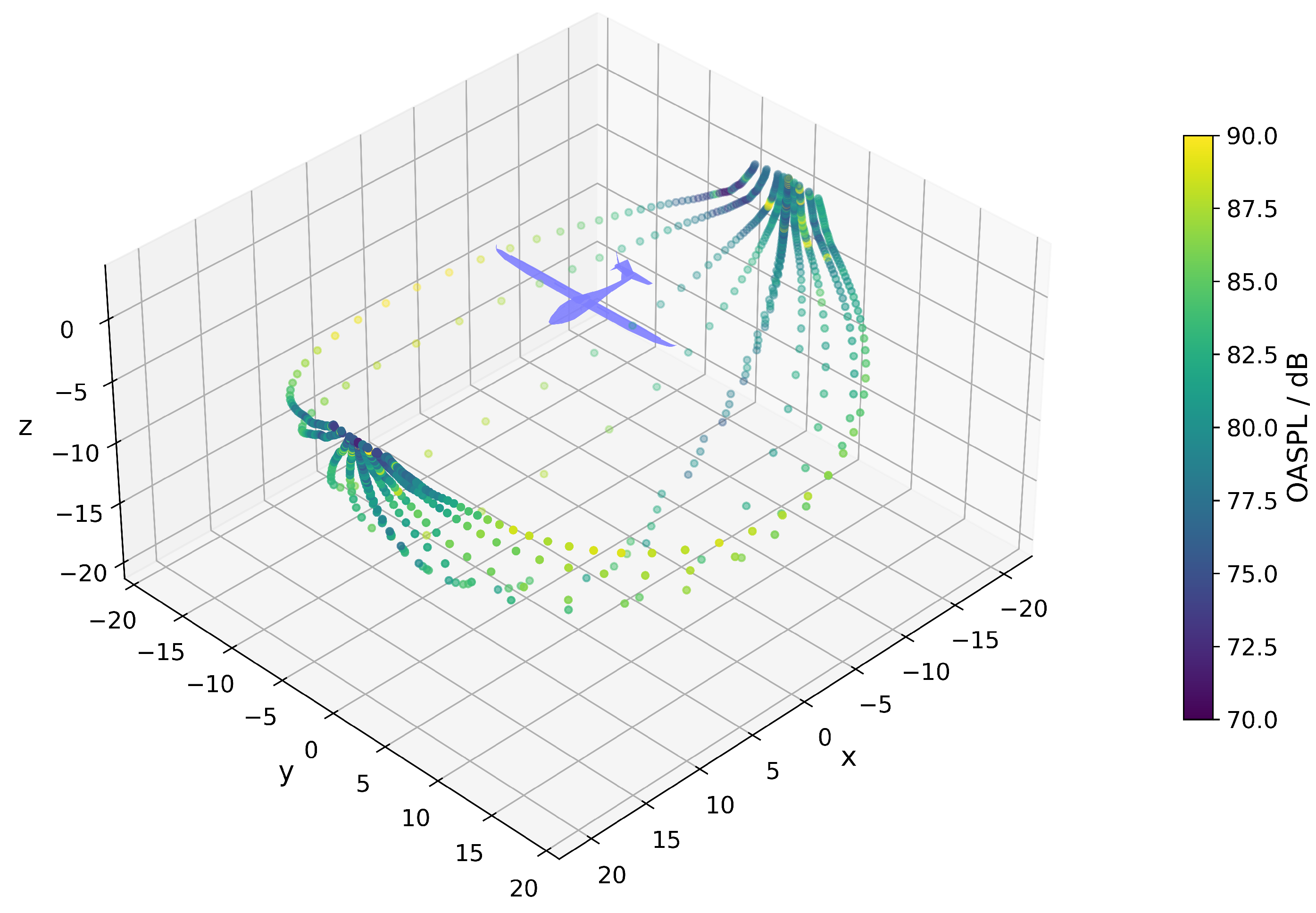
OASPL hemisphere extracted from all twelve microphones and 99 FFTs for incident 11, flight 1, given relative to a reference radius of 20 m. The orientation of the aircraft is given by the transparent model drawn to scale, with the center of the hemisphere assumed at x = 25% Mean Aerodynamic Chord on the longitudinal axis.
Figure 7.
OASPL hemisphere extracted from all twelve microphones and 99 FFTs for incident 11, flight 1, given relative to a reference radius of 20 m. The orientation of the aircraft is given by the transparent model drawn to scale, with the center of the hemisphere assumed at x = 25% Mean Aerodynamic Chord on the longitudinal axis.
Figure 8.
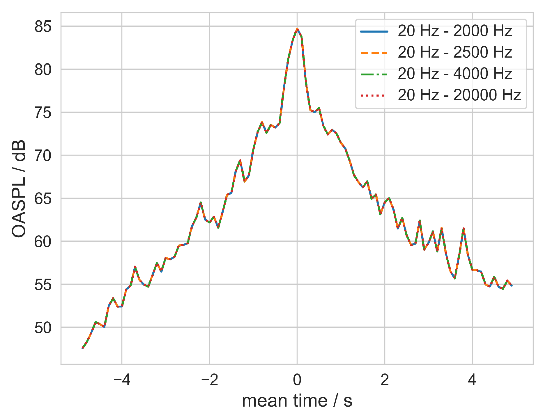
OASPL over one overflight (incident 11 of recording 1) for different one-third-octave band upper limits. The influence of higher frequencies on the OASPL is negligible, as can be seen by the coinciding lines.
Figure 8.
OASPL over one overflight (incident 11 of recording 1) for different one-third-octave band upper limits. The influence of higher frequencies on the OASPL is negligible, as can be seen by the coinciding lines.
Figure 9.
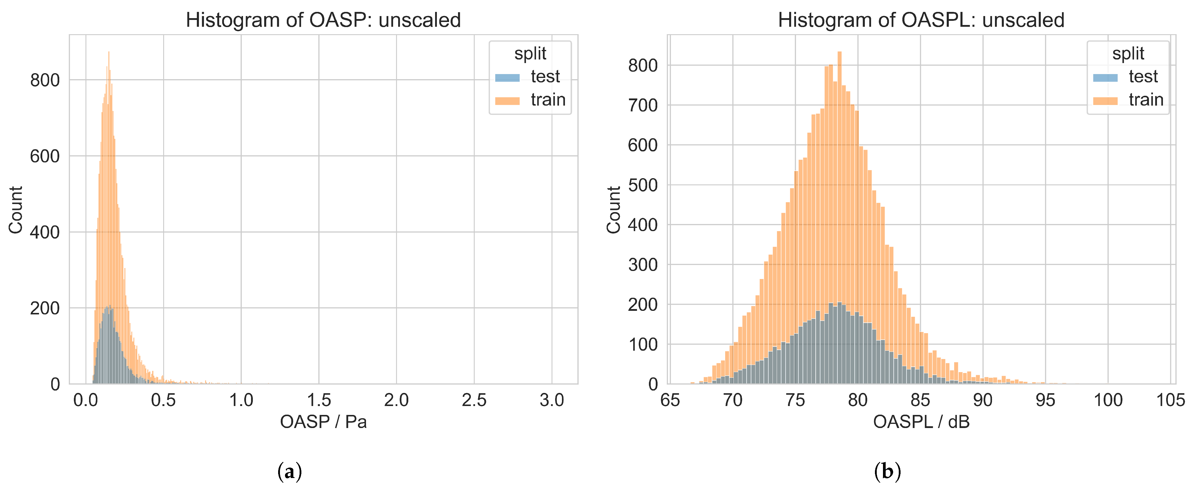
Comparison of the histograms of OASP and OASPL for all overflights in the data set. Test data in blue and training data in orange. (a) Histogram of unscaled OASP in Pa, with minimum 0.0428 Pa and maximum 3.018 Pa. (b) Histogram of unscaled OASPL in dB, with minimum 66.61 dB and maximum 103.58 dB.
Figure 9.
Comparison of the histograms of OASP and OASPL for all overflights in the data set. Test data in blue and training data in orange. (a) Histogram of unscaled OASP in Pa, with minimum 0.0428 Pa and maximum 3.018 Pa. (b) Histogram of unscaled OASPL in dB, with minimum 66.61 dB and maximum 103.58 dB.
Figure 10.
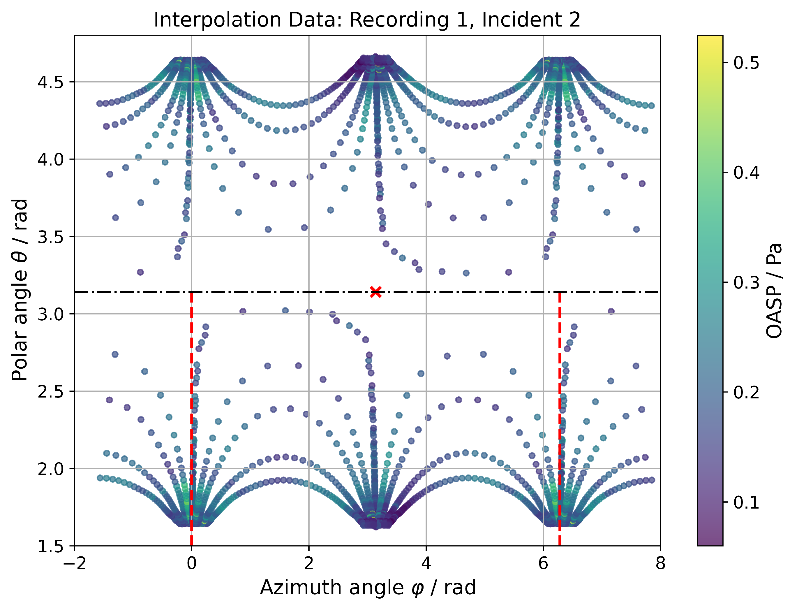
Resulting data after mirroring and reflection to account for singularity and periodicity for one exemplary overflight. The original data and interpolations are in the range and . Mirroring for periodicity is shown with the red dashed lines, and the point reflection due to the singularity is shown by the x marker. In addition, the dash–dot line is shown to highlight the singularity.
Figure 10.
Resulting data after mirroring and reflection to account for singularity and periodicity for one exemplary overflight. The original data and interpolations are in the range and . Mirroring for periodicity is shown with the red dashed lines, and the point reflection due to the singularity is shown by the x marker. In addition, the dash–dot line is shown to highlight the singularity.
Figure 11.
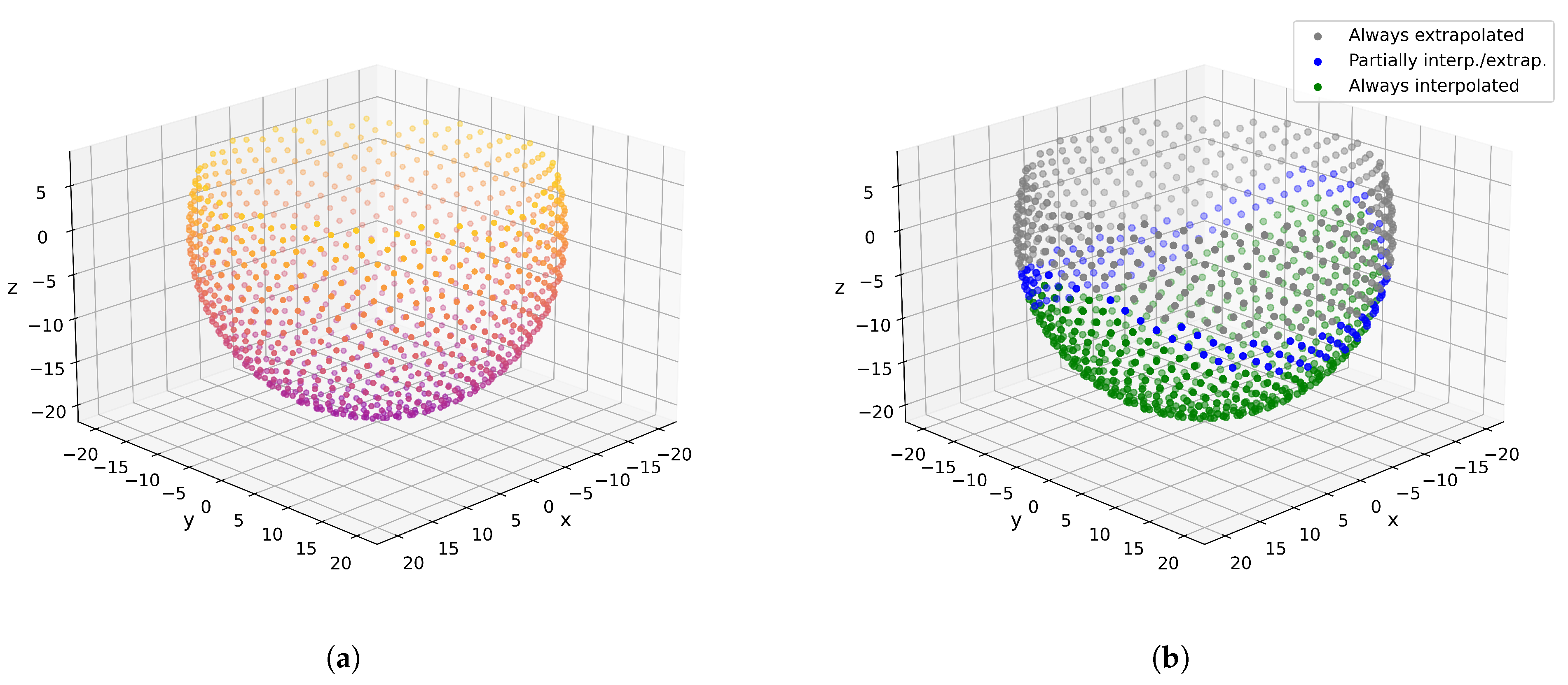
Fibonacci sphere and the (partially) extrapolated points. (a) Virtual microphones on the Fibonacci sphere, cut 20° above the horizon. The color gradient highlights the z-value. (b) Always-extrapolated values (gray), partially interpolated/extrapolated values (blue), and always-interpolated values (green) on the Fibonacci sphere based on all overflights.
Figure 11.
Fibonacci sphere and the (partially) extrapolated points. (a) Virtual microphones on the Fibonacci sphere, cut 20° above the horizon. The color gradient highlights the z-value. (b) Always-extrapolated values (gray), partially interpolated/extrapolated values (blue), and always-interpolated values (green) on the Fibonacci sphere based on all overflights.
Figure 12.
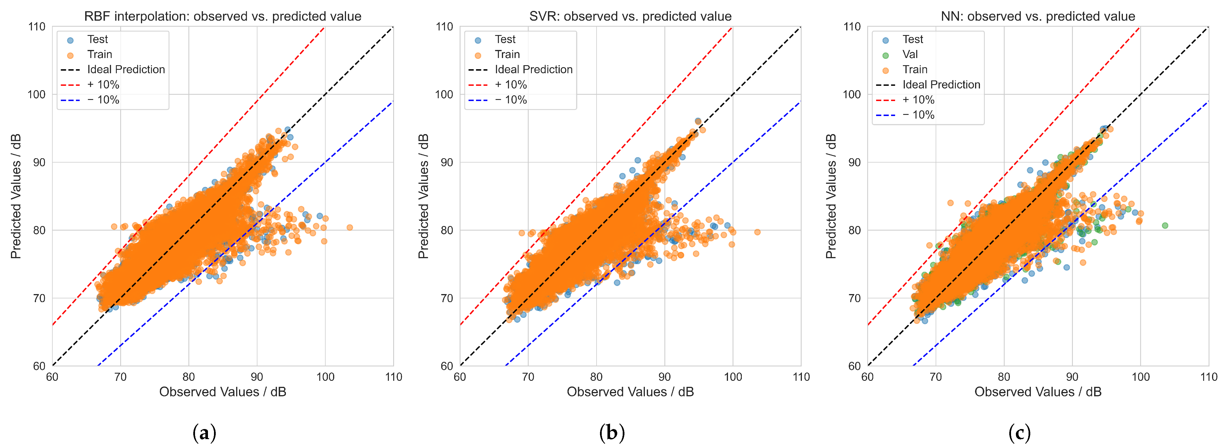
Predicted values versus observed values for the RBF interpolation, SVR, and NN models. Training data are shown in orange, test data in blue, and NN validation data in green. The black dashed line is the ideal prediction, red is +10% and blue is −10%. Sub-figures: (a) RBF interpolation, (b) SVR, and (c) NN.
Figure 12.
Predicted values versus observed values for the RBF interpolation, SVR, and NN models. Training data are shown in orange, test data in blue, and NN validation data in green. The black dashed line is the ideal prediction, red is +10% and blue is −10%. Sub-figures: (a) RBF interpolation, (b) SVR, and (c) NN.
Figure 13.
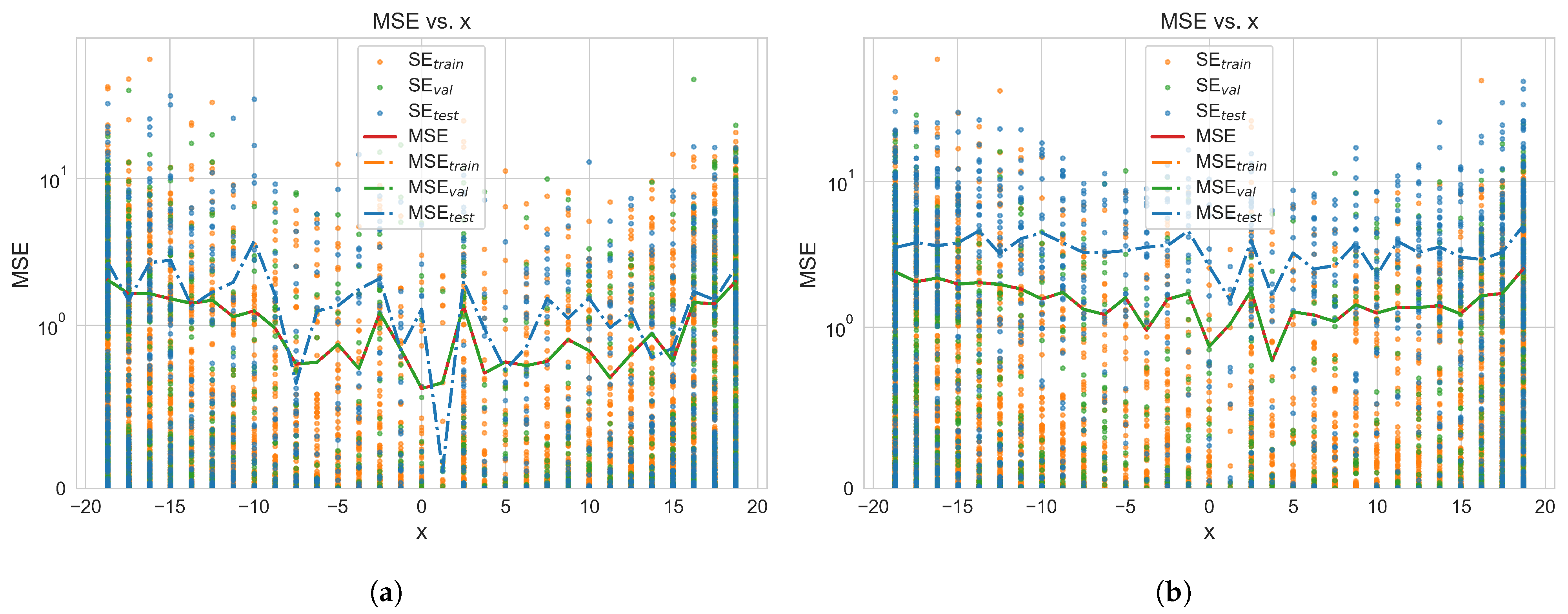
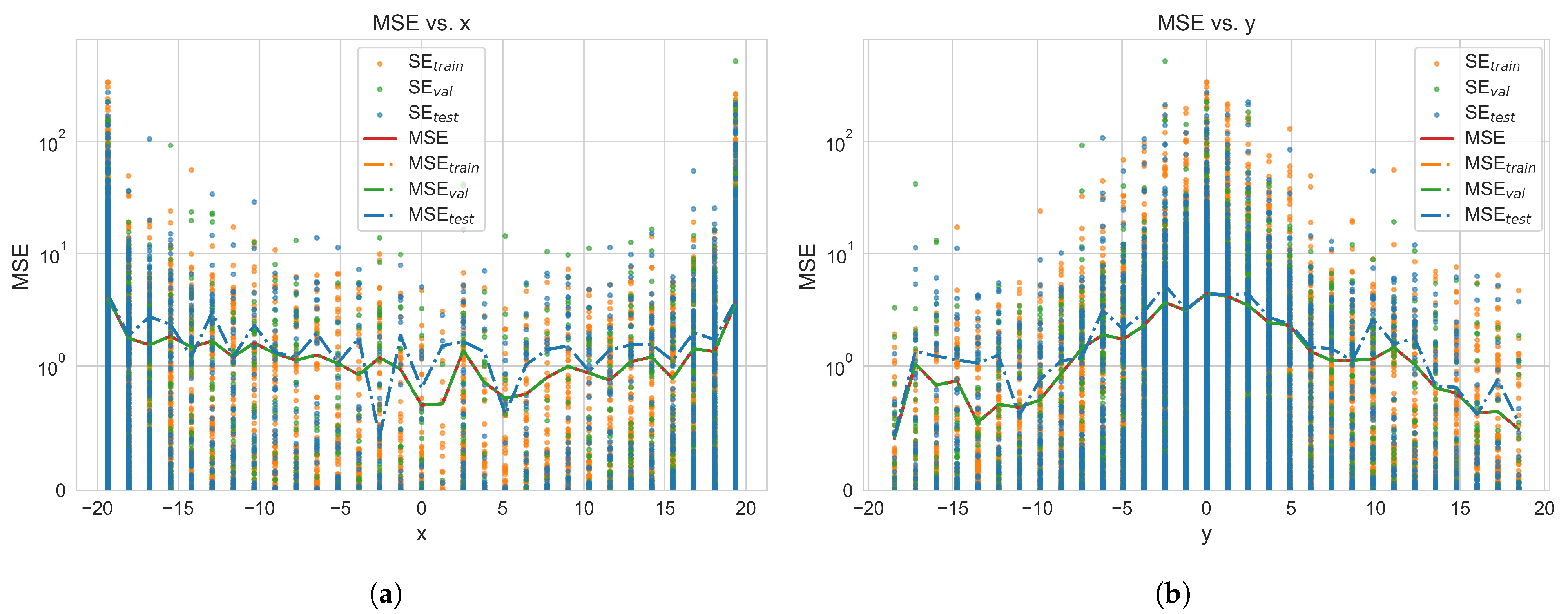
The graphs show the squared error (SE) and its mean for bins across the x- and y-coordinates. The results for the NN model are the ones displayed; however, the other approaches lead to similar results. Sub-figures: (a) MSE vs. x-coordinate, and (b) MSE vs. y-coordinate.
Figure 13.
The graphs show the squared error (SE) and its mean for bins across the x- and y-coordinates. The results for the NN model are the ones displayed; however, the other approaches lead to similar results. Sub-figures: (a) MSE vs. x-coordinate, and (b) MSE vs. y-coordinate.
Figure 14.
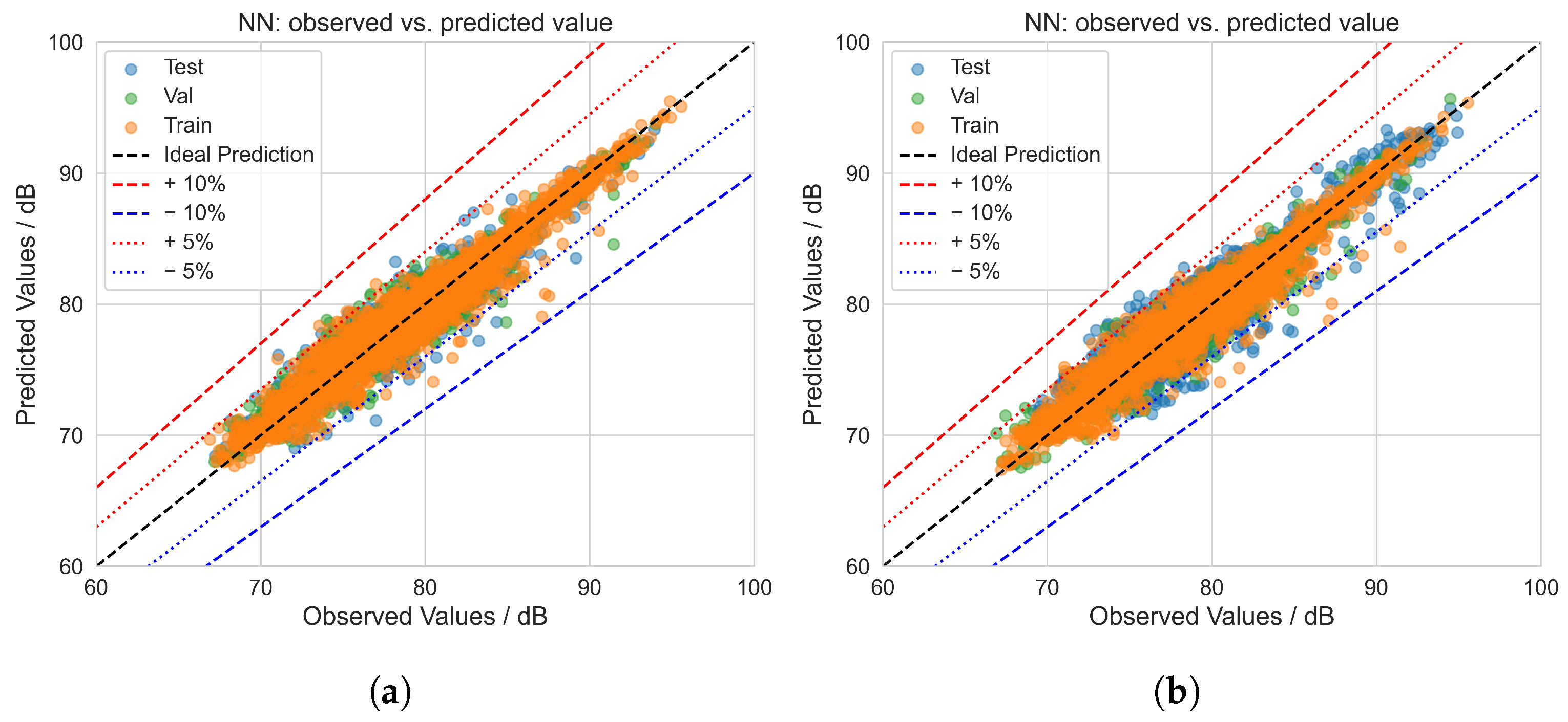
Predicted values versus observed values for both NN splitting variants. Training data are shown in orange, validation data in green, and test data in blue. The black dashed line is the ideal prediction, whereas red is +10% or +5% and blue is −10% or −5%. Sub-figure: (a) standard splitting approach, (b) splitting by overflight.
Figure 14.
Predicted values versus observed values for both NN splitting variants. Training data are shown in orange, validation data in green, and test data in blue. The black dashed line is the ideal prediction, whereas red is +10% or +5% and blue is −10% or −5%. Sub-figure: (a) standard splitting approach, (b) splitting by overflight.
Figure 15.
The figures show the squared error (SE) and its mean for bins over the x-coordinates for both splitting options. The sub figure (a) is for the standard split, and (b) is for the overflight split.
Figure 15.
The figures show the squared error (SE) and its mean for bins over the x-coordinates for both splitting options. The sub figure (a) is for the standard split, and (b) is for the overflight split.
Figure 16.
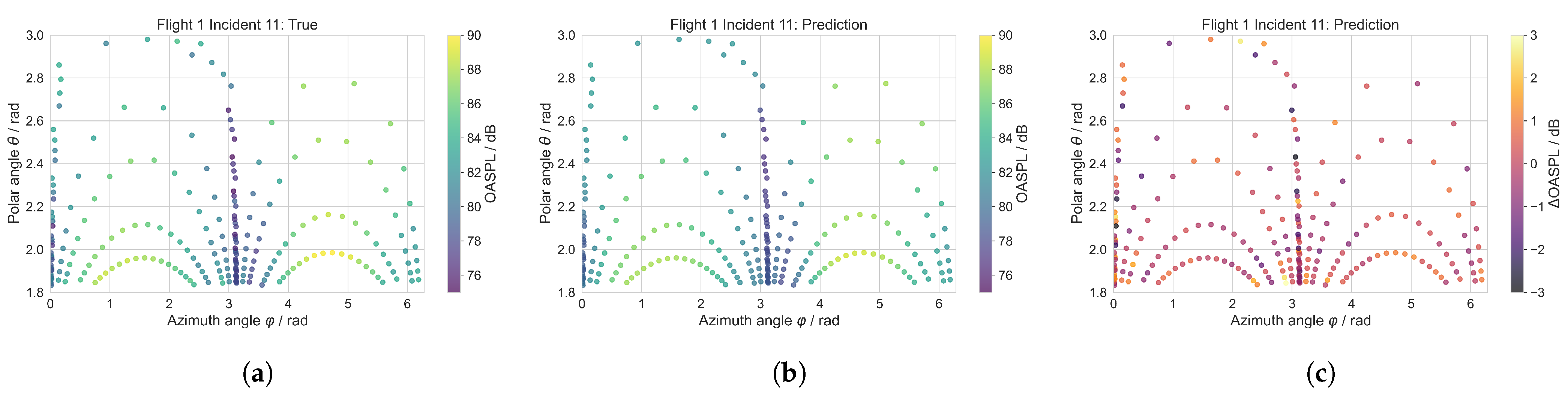
Overview of the experimental results, predictions by the standard split NN, and absolute ΔOASPL. Sub-figures: (a) experimental results, (b) predictions, (c) ΔOASPL.
Figure 16.
Overview of the experimental results, predictions by the standard split NN, and absolute ΔOASPL. Sub-figures: (a) experimental results, (b) predictions, (c) ΔOASPL.
Table 1.
Metrics of the LR models with the lowest MSEval for each model, where MSE is given in the scaled frame and MSEdB is given as OASPL in dB. All best models are with Cartesian coordinates and OASPL for training.
Table 1.
Metrics of the LR models with the lowest MSEval for each model, where MSE is given in the scaled frame and MSEdB is given as OASPL in dB. All best models are with Cartesian coordinates and OASPL for training.
| Model | MSEtrain | MSEval | MSEdB, train | MSEdB, val |
|---|
| Lin. Reg. | 0.601922 | 0.602615 | 9.946525 | 9.957974 |
| Lasso | 0.601922 | 0.602615 | 9.946527 | 9.957974 |
| Ridge | 0.601924 | 0.602609 | 9.946554 | 9.957883 |
| ElasticNet | 0.601927 | 0.602609 | 9.946605 | 9.957875 |
Table 2.
Metrics of the RBF interpolation model with the lowest MSEdB, val for each kernel. All models are based on Cartesian coordinates and OASPL.
Table 2.
Metrics of the RBF interpolation model with the lowest MSEdB, val for each kernel. All models are based on Cartesian coordinates and OASPL.
| Kernel | MSEtrain | MSEval | MSEdB, train | MSEdB, val |
|---|
| Linear | 0.089 | 0.200 | 1.472 | 3.307 |
| TPS 1 | 0.145 | 0.204 | 2.399 | 3.367 |
| Cubic | 0.142 | 0.208 | 2.351 | 3.445 |
| Quintic | 0.169 | 0.221 | 2.790 | 3.656 |
| MQ 2 | 0.137 | 0.202 | 2.270 | 3.339 |
| IQ 3 | 0.175 | 0.224 | 2.896 | 3.698 |
| IMQ 4 | 0.091 | 0.218 | 1.507 | 3.598 |
| Gaussian | 0.208 | 0.231 | 3.429 | 3.825 |
Table 3.
Metrics of the selected RBF interpolator model (Cartesian coordinates, quintic kernel, StandardScaler, and OASPL). Training and validation metrics are the mean of all CV folds. All test metrics are calculated for a model retrained on the whole training set, resulting in improvement over validation metrics.
Table 3.
Metrics of the selected RBF interpolator model (Cartesian coordinates, quintic kernel, StandardScaler, and OASPL). Training and validation metrics are the mean of all CV folds. All test metrics are calculated for a model retrained on the whole training set, resulting in improvement over validation metrics.
| | MSEtrain | MSEval | R2train | R2val | MSEtest | MAEtest | R2test |
|---|
| Scaled | 0.273 | 0.278 | 0.727 | 0.722 | 0.272 | 0.373 | 0.719 |
| OASPL | 4.514 | 4.595 | 0.727 | 0.722 | 4.495 | 1.516 | 0.719 |
Table 4.
Rank correlations of the selected RBF interpolator model (Cartesian coordinates, quintic kernel, StandardScaler, and OASPL) calculated on the final model, where the training set is the whole set without any validation data. Rank correlation is unaffected by scaling.
Table 4.
Rank correlations of the selected RBF interpolator model (Cartesian coordinates, quintic kernel, StandardScaler, and OASPL) calculated on the final model, where the training set is the whole set without any validation data. Rank correlation is unaffected by scaling.
| | | | | |
|---|
| 0.853 | 0.842 | 0.851 | 0.673 | 0.663 | 0.671 |
Table 5.
Metrics of the SVR model with the lowest MSEdB, val for each kernel. All models are based on Cartesian coordinates and OASPL.
Table 5.
Metrics of the SVR model with the lowest MSEdB, val for each kernel. All models are based on Cartesian coordinates and OASPL.
| Kernel | MSEtrain | MSEval | MSEdB, train | MSEdB, val |
|---|
| Linear | 0.603 | 0.603 | 9.958 | 9.970 |
| RBF | 0.241 | 0.250 | 3.985 | 4.135 |
| 2nd Poly. | 0.402 | 0.403 | 6.635 | 6.658 |
| 3rd Poly. | 0.323 | 0.326 | 5.339 | 5.387 |
| 4th Poly. | 0.281 | 0.285 | 4.642 | 4.709 |
| 5th Poly. | 0.267 | 0.273 | 4.415 | 4.505 |
| 6th Poly. | 0.257 | 0.265 | 4.253 | 4.371 |
Table 6.
Metrics of the selected SVR model (Cartesian coordinates, RBF kernel, StandardScaler, and OASPL). Training and validation metrics are the mean of all CV folds. All test metrics are calculated with a model retrained on the whole training set, resulting in improvement over validation metrics.
Table 6.
Metrics of the selected SVR model (Cartesian coordinates, RBF kernel, StandardScaler, and OASPL). Training and validation metrics are the mean of all CV folds. All test metrics are calculated with a model retrained on the whole training set, resulting in improvement over validation metrics.
| | MSEtrain | MSEval | R2train | R2val | MSEtest | MAEtest | R2test |
|---|
| scaled | 0.241 | 0.250 | 0.759 | 0.750 | 0.247 | 0.340 | 0.745 |
| OASPL | 3.985 | 4.135 | 0.759 | 0.750 | 4.074 | 1.380 | 0.745 |
Table 7.
Rank correlations of the selected SVR model (Cartesian coordinates, RBF kernel, StandardScaler, and OASPL) calculated on the final model, where the training set is the whole set without any validation data. Rank correlation is unaffected by scaling.
Table 7.
Rank correlations of the selected SVR model (Cartesian coordinates, RBF kernel, StandardScaler, and OASPL) calculated on the final model, where the training set is the whole set without any validation data. Rank correlation is unaffected by scaling.
| | | | | |
|---|
| 0.875 | 0.862 | 0.872 | 0.704 | 0.689 | 0.701 |
Table 8.
Metrics of the selected NN model. Training and validation metrics are given at the epoch where the minimal validation loss occurs. Test metrics are calculated on the same model.
Table 8.
Metrics of the selected NN model. Training and validation metrics are given at the epoch where the minimal validation loss occurs. Test metrics are calculated on the same model.
| | MSEtrain | MSEval | R2train | R2val | MSEtest | MAEtest | R2test |
|---|
| Scaled | 0.187 | 0.202 | 0.762 | 0.741 | 0.213 | 0.321 | 0.720 |
| OASPL | 3.095 | 3.337 | 0.762 | 0.741 | 3.516 | 1.306 | 0.720 |
Table 9.
Rank correlations of the selected NN model for the final model; training metrics are given for the full training set (including validation data). Rank correlation is unaffected by scaling.
Table 9.
Rank correlations of the selected NN model for the final model; training metrics are given for the full training set (including validation data). Rank correlation is unaffected by scaling.
| | | | | |
|---|
| 0.901 | 0.881 | 0.897 | 0.738 | 0.713 | 0.733 |
Table 10.
Metrics of the NN model with standard split. Training and validation metrics are given at the epoch where the minimal validation loss occurs.
Table 10.
Metrics of the NN model with standard split. Training and validation metrics are given at the epoch where the minimal validation loss occurs.
| Metric | Frame | Train | Val | Test |
|---|
| MSE | Scaled | 0.057 | 0.084 | 0.090 |
| | OASPL | 1.192 | 1.750 | 1.880 |
| MAE | scaled | 0.174 | 0.213 | 0.225 |
| | OASPL | 0.795 | 0.978 | 1.028 |
| R2 | – | 0.938 | 0.910 | 0.896 |
| – | 0.962 | 0.940 | 0.937 |
| – | 0.843 | 0.801 | 0.793 |
Table 11.
Metrics of the NN model with overflight split. Training and validation metrics are given at the Epoch where the minimal validation loss occurs.
Table 11.
Metrics of the NN model with overflight split. Training and validation metrics are given at the Epoch where the minimal validation loss occurs.
| Metric | Frame | Train | Val | Test |
|---|
| MSE | Scaled | 0.059 | 0.081 | 0.175 |
| | OASPL | 1.244 | 1.692 | 3.673 |
| MAE | Scaled | 0.175 | 0.215 | 0.339 |
| | OASPL | 0.799 | 0.983 | 1.552 |
| R2 | – | 0.935 | 0.918 | 0.802 |
| – | 0.961 | 0.952 | 0.837 |
| – | 0.842 | 0.818 | 0.652 |