Servo-Elastic Control of a Flexible Airship with Multiple Vectored Propellers

Abstract

Owing to its large flexible envelope, an airship is highly sensitive to environmental disturbances, such as wind gusts. Fluid–structure interaction induces structural deformation, which modifies the aerodynamic force distribution and introduces additional coupling effects. Furthermore, servo-elastic deformation alters the position and orientation of actuators mounted on the envelope, resulting in deviations between commanded and actual control forces. To address these issues, a composite control strategy integrating trajectory tracking and active elastic deformation suppression is proposed for a flexible airship equipped with multiple vectored propellers. Structural flexibility is explicitly incorporated into the dynamic model through modal decomposition, where the generalized coordinates and their time derivatives associated with deformation modes are included in the system state vector. A disturbance observer is developed to estimate actuator-level force deviations induced by elastic deformation, and the estimated disturbances are compensated in real time. Based on this formulation, a composite control framework, referred to as servo-elastic control, is established. The framework consists of a trajectory tracking controller and a displacement compensation module to achieve simultaneous motion regulation and structural deflection suppression. Numerical results demonstrate that the displacement at vectored thrust actuator attachment points is reduced to approximately 10% of that obtained using a trajectory tracking controller alone. The proposed method achieves significant deformation suppression without degrading position tracking performance, thereby enhancing control effectiveness and system stability of flexible airships.

1. Introduction

Airships offer significant advantages, including a large payload capacity and the ability to hover in the sky, making them promising for applications such as disaster rescue and Earth observation [1,2]. However, their large size and lighter-than-air nature result in a flexible body and susceptibility to environmental factors, posing challenges for effective control. Therefore, enhancing control mechanisms remains a primary focus in airship research [3].

The earliest research on modeling flexible airships began with analyzing the static deformation of airships using simple beam models [4], followed by modeling the influence of deformation on inertial forces [5]. With the improvement of computing power, finite element analysis (FEA) and computational fluid dynamics (CFD) have become critical tools for analyzing both static deformation and aerodynamic forces of large flexible airships. Jianming Liu [6] proposed a computational method to analyze the large deformations of membrane structures in a three-dimensional flow field, considering the impact of flight parameters on the deformation of airships and their aerodynamic coefficients. Maohua Zhang [7] developed a combination of finite element and engineering estimation methods to calculate aerodynamic forces, as well as a numerical panel method to determine the added mass for flexible airships with arbitrary shapes. Subsequent in-depth research has focused on the effects of fluid–structure–thermal interactions on aerodynamics [8]. Yuwen Li was the first to present a complete process for establishing the fluid–structure interaction equations for airships, integrating flight dynamics, structural dynamics, aerodynamics, and aerostatics [9].

Despite the various approaches currently employed to study the fluid–structure interaction characteristics of airships, existing control theories primarily rely on rigid models [10,11] or treat the nonlinear aspects of fluid–structure coupling as perturbations [12,13]. These studies fail to account for the counteracting effects of elastic deformation and vibrations on the actuators [14,15]. Current theories on servo-elastic control for aerospace systems primarily focus on aerodynamic servo-elasticity in airplanes and missiles [16,17,18], whereas traditional methods rely on aerodynamic fins to address structural vibrations locally, often focusing on avoiding flutter through gain scheduling [19,20].

However, the servo-elastic behavior of airships differs fundamentally from conventional aircraft due to three distinct characteristics. First, given their low flight speeds, which render traditional aerodynamic surfaces inefficient, airships rely on multiple vectored propellers not only to enhance control accuracy but also as the primary mechanism for suppressing servo-elastic instabilities [21]. Second, their lightweight envelope structures, maintained by internal pressure differentials rather than rigid frames, exhibit high sensitivity to altitude variations, external airflow, gas exchange, and thermodynamic conditions, all of which significantly govern their elastic dynamics [22]. Finally, at such low speeds, ambient wind emerges as a dominant disturbance; under these conditions—characterized by low dynamic pressure alongside high angles of attack and large sideslip angles—the coupling between structural flexibility and flight control systems becomes particularly critical [23].

Airship development has progressed relatively slowly, and as a result, little work has been done on flutter and divergence in large flexible airships. Consequently, there is currently no publicly available servo-elastic control theory specifically designed for such vehicles. To achieve satisfactory control performance—particularly for giant flexible airships—it would be essential to explicitly account for fluid–structure coupling effects.

The main contributions of this work are twofold. First, a novel fluid–structure interaction (FSI) modeling framework is established, which rigorously couples structural deformation with aerodynamics derived from fluid mechanics. Unified equations are formulated to integrate deformed structural mechanics with flight dynamics, explicitly accounting for the control implications of servo-actuator installation offsets and attitude deviations caused by large elastic deformations. Second, building on this high-fidelity model, the use of vectored propellers as the primary mechanism to suppress structural vibrations in large flexible airships is proposed for the first time. While traditional methods rely on aerodynamic fins to address structural vibrations locally, global active suppression of structural modes is achieved in this framework by directly utilizing vectored thrust. Unlike conventional approaches that lose effectiveness at low speeds, the structural deformation of the entire vehicle is controlled independent of aerodynamic forces, offering a new and robust way to stabilize giant flexible airships.

The remainder of this paper is organized as follows: Section 2 details the flexible deformation model and the derivation of aerodynamic and thrust forces under FSI conditions. Section 3 presents the design of the servo-elastic controller and the disturbance estimator, accompanied by stability analysis. Section 4 demonstrates the feasibility of the proposed design through simulation results, analyzing potential issues within the control system and offering insights for subsequent developments.

2. Dynamics of Flexible Airships

In this paper, a high-altitude unmanned airship is proposed, designed to operate at an altitude of 20 km. The airship has a length of 50 m, with a maximum cross-sectional diameter of 10 m, a volume of 5219 m³, and a mass of 2682 kg. There is a gondola beneath the airship. The elevator and the rudder are located in the stern of the body. There are three propellers on each side, arranged in a fore–mid–aft configuration along the circumference line, as shown in Figure 1. The origin of the airship’s body-fixed coordinate system $o_b{x}_b{y}_b{z}_b$ is located at the volume center of the airship, with the $x_b$-axis aligned along the longitudinal axis and the $z_b$-axis pointing vertically downward. The local frame of vectored thrust $o_p{x}_p{y}_p{z}_p$ is established in the vectored-rotation plane, in which the vectored propeller can deflect about the vectored axis at a range of $[-90°,90°]$. The vectored angle of each propeller is denoted by ${\mu }_i (i=1,2,3,4,5,6)$, and the generated force is represented by $f_i (i=1,2,3,4,5,6)$. Each propeller has a maximum thrust of 500 N. The main parameters of this airship are given in

Table 1. Main parameters of airship.

Mounting Position of Propellers (m)	Added Mass and Moments (kg) or (kg.m2)
[x1,y1,z1] = [17,8,0] [x2,y2,z2] = [−4,9,0] [x3,y3,z3] = [−15,7,0] [x4,y4,z4] = [17,−8,0] [x5,y5,z5] = [−4,−9,0] [x6,y6,z6] = [−15,−7,0]	m11 = 5.1 × 102 m22 = m33 = 5.07 × 103 m44 = 6.88 × 104 m55 = m66 = 5.85 × 105 m26 = −m35 = 1.29 × 104
Mass and inertia (kg) or (kg.m2)	Coefficients of control surfaces (1/deg)
m0 = 2682, Ix = 1.07 × 105, Iy = 2.82 × 105, Iz = 2.11 × 105, Ixy = 0, Ixz = 70, Iyz = 0	$c_{\delta }$ = 6.5 × 10−3
Volume of the airship	Position of gravity center (m)
Vol = 5219 m3	$[x_G,y_G,z_G]$ = [0,0,1.898].

.

2.1. Deformation Analysis of a Flexible Airship

As mentioned above, deformation can significantly affect the aerodynamic performance of the airship and the efficiency of its propulsion system. To establish a dynamic model for a flexible airship, it is crucial to accurately characterize the deformation that occurs during flight. Since this deformation results from the combined effects of external aerodynamic forces, internal pressure differentials, and ambient wind conditions, it must be captured through an iterative fluid–structure interaction (FSI) approach. In this work, the FSI simulations are carried out using the ANSYS Workbench 2022 R2 platform.

2.1.1. Typical Mode Shapes

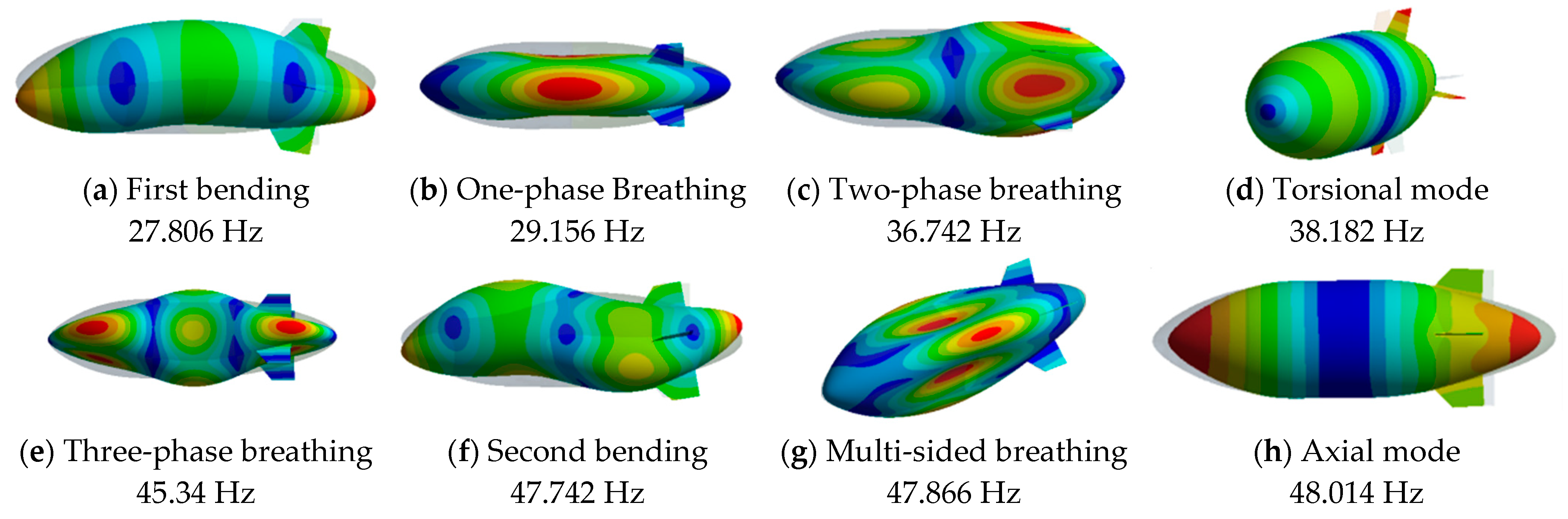
Prior to the transient FSI simulation, a Static Structural Analysis module is first performed with prescribed pressure differential 500 Pa at 216.5 K to account for the stiffness contribution of internal pressure. The resulting deformed equilibrium state is used as the reference configuration for a subsequent modal analysis module. This ensures that the natural frequencies and mode shapes reflect the actual operational stiffness of the inflated envelope, which is critical for control-oriented modeling. The modal analysis results identify several key modes, as illustrated in Figure 2 [23].

These mode shapes describe how the structure deforms at specific frequencies, which is essential for understanding the airship’s dynamic behavior during flight. The identified modes are categorized into two main types: global modes and local modes. The global modes include (a), (d), (f) and (h), and their frequencies are not significantly affected by pressure differences. The local modes include various forms of breathing modes, which are greatly influenced by pressure differences [24]. Local modes are crucial for understanding hull deformation under varying pressure conditions, whereas global modes are more relevant to large-scale flight dynamics, which in turn affect both aerodynamic performance and propulsion efficiency.

2.1.2. Envelope Deformation Model

In the body coordinate system, the modal shape of a specific mode at a given node can be represented in vector form as ${\zeta }_{ji}={\left[\begin{array}{ccc}{\zeta }_{jix}& {\zeta }_{jiy}& {\zeta }_{jiz}\end{array}\right]}^{\mathrm{T}}$, where the subscript $j=1\dots m$ refers to the mode order, the subscript $i=1\dots n$ refers to the number of nodes, and ${\zeta }_{ji}$ is the modal shape vector, representing the relative displacement of the i node along the three axes of the body-fixed coordinate system in the j-th mode. The modal shape vectors for a specific node i across modes 1 to m can be written as: ${\Phi }_i={\left[\begin{array}{cccc}{\zeta }_{1i}& {\zeta }_{2i}& \dots & {\zeta }_{mi}\end{array}\right]}_{3\times m}$, and the full modal shape matrix containing all nodes is denoted by $\Psi ={\left[\begin{array}{cccc}{\Phi }_1& {\Phi }_2& \dots & {\Phi }_n\end{array}\right]}_{3n\times m}^{\mathrm{T}}$. The modal shape matrix represents the spatial deformation patterns (or mode shapes) associated with each natural frequency of the airship’s flexible dynamics. Generalized variables are used to describe the time history of the vibration state of a dynamic system and are typically expressed as: $q={\left[\begin{array}{cccc}{q}_1& q_2& \dots & q_m\end{array}\right]}^{\mathrm{T}}$, which can be solved through the fluid–structure interaction dynamic equations presented in Section 2.5. By performing modal analysis and formulating the equations of elastic motion, the dynamic deformation data of the airship is expressed as

$$D=\Psi q$$

(1)

where $D={\left[\begin{array}{cccc}{d}_1& d_2& \dots & d_n\end{array}\right]}^{\mathrm{T}}$ is the deformation of the airship. For each node i, the displacement components along the three axes in the body-fixed coordinate system are represented by the vector $d_i={\left[\begin{array}{ccc}{d}_{ix}& d_{iy}& d_{iz}\end{array}\right]}^{\mathrm{T}}$ with

$$d_i={\Phi }_{i}q$$

(2)

2.2. FSI-Based Aerodynamic Modeling Framework

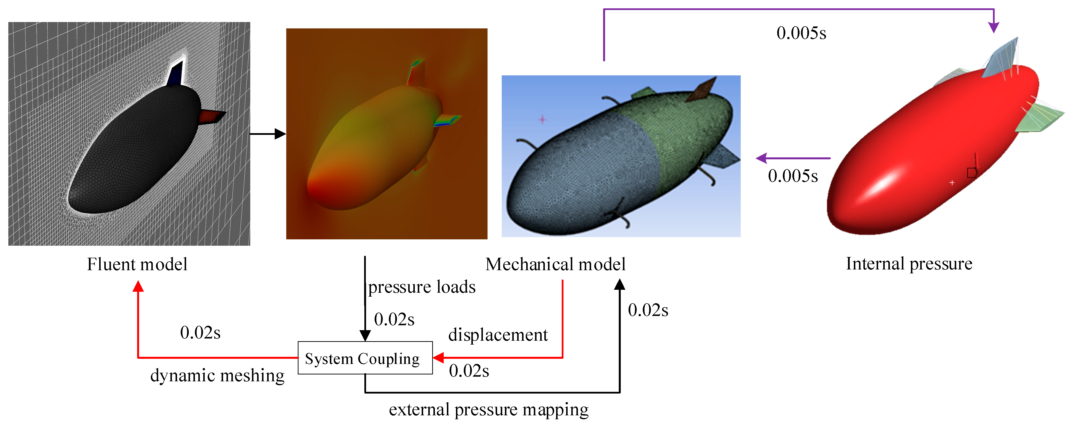
While the structural displacement field is efficiently parameterized using a linear superposition of dominant mode shapes, the proposed FSI framework rigorously accounts for geometric nonlinearities associated with large deformations. This is achieved by continuously updating the structural stiffness matrix and the fluid domain mesh based on the instantaneous large-deformed configuration at each time step. Consequently, to ensure a high-precision aerodynamic representation, the aerodynamic coefficients under deformation are derived directly through these FSI calculations. The FSI analysis framework is shown in Figure 3. A strongly coupled partitioned FSI scheme is employed via the System Coupling module: the ANSYS Fluent module solves the transient compressible external flow field, while the ANSYS Mechanical module computes the large-deformation structural response of the flexible envelope. In the Internal pressure model, internal gas dynamics are fully resolved via the ideal gas law. While the framework supports transient thermal analysis, we apply a quasi-steady thermal assumption here. Since external temperature changes are much slower than structural responses, we treat internal temperature as constant per operating condition. Within each global coupling time step (Δt = 0.02 s), multiple iterations are performed between the two solvers until convergence of both interface displacements and fluid loads is achieved.

This Workbench-based FSI framework provides a physically consistent and numerically stable platform for capturing the aerodynamic behavior under fluid–structure interaction and for developing a dynamic model of the coupled system. The key simulation modules are configured as follows:

Fluid Domain and Meshing: The external flow is simulated in ANSYS Fluent using a polyhedral mesh generated with Fluent Meshing, which provides high solution accuracy while reducing the total cell count compared to conventional tetrahedral meshes. A 5-layer prism boundary layer mesh is applied near the airship surface, targeting a dimensionless wall distance of y + ≈ 100. Far-field boundaries are positioned at least 20 times the airship length away from the body, configured as a velocity inlet and a pressure outlet. The simulation employs the k–ω SST turbulence model, and a transient pressure-based coupled solver with a time step of Δt = 0.02 s. While the ideal gas law is used to maintain solver generality, the low mach number (Ma < 0.3) ensures that density variations are negligible, effectively treating the flow as incompressible. Propeller effects are modeled using a nested sliding mesh approach. Thrust computation utilizes the Multiple Reference Frame (MRF) method for steady-state initialization and the Sliding Mesh (SM) technique for transient interactions, where SM models the propeller’s motion around the airship and MRF handles its self-rotation. Actuator disk locations are defined directly on the deformable envelope surface to account for structural motion during flight.

Structural Model Details: The airship envelope (skin) is modeled as a membrane using triangular SHELL181 elements with a characteristic size of 0.5 m and bending stiffness is neglected. The material is assumed isotropic with Young’s modulus E = 3.1 × 10⁹ Pa, Poisson’s ratio ν = 0.42, and an areal density of 90 g/m². The tail fins are discretized with tetrahedral Solid 226 elements (element size ranging from 0.1 to 0.5 m). The connection between the tail and the envelope is reinforced using BEAM188 beam elements (0.5 m size) and is modeled in ANSYS Workbench with a bonded (tie) contact condition. The gondola (pod) is simplified as four fixed support points to represent its rigid mounting to the envelope.

The structural solver uses a sampling interval of 0.005 s (corresponding to a sampling frequency of 200 Hz) to adequately resolve the dynamic characteristics of the first eight structural vibration modes. As shown in Figure 2, the dominant frequencies from modal analysis are approximately 50 Hz. After advancing through four subcycles (totaling 0.02 s), the resulting deformation field is transferred from the Mechanical module to the System Coupling interface. The FSI coupling loop operates with a macro time step of 0.02 s, synchronized with the transient fluid solver in Fluent. The structural solver was set to perform 25 iterations per coupling step by default. In Fluent, the number of iterations per time step was determined based on the convergence of the monitored variables. Initially, more iterations were required, up to 35, but as the simulation progressed, fewer iterations were needed, and typically convergence was achieved within 5–6 iterations per time step on average.

FSI Data Transfer: The computational model comprises three coupled domains: the structural hull, an inner fluid layer, and an outer fluid field. Shared topology is applied at the interface between the inner and outer fluid domains, merging their nodes to ensure seamless data continuity without interpolation. At the fluid–structure interfaces, distinct transfer strategies are employed: internal pressure loads from the inner fluid are directly mapped onto the structure (leveraging conformal meshing), whereas external aerodynamic loads from the outer flow are transferred via conservative interpolation to accommodate non-matching meshes. Both load types are applied as surface traction boundary conditions. Conversely, structural nodal displacements are interpolated to drive the fluid boundaries. To support these movements, dynamic meshing, combining spring-based smoothing and local remeshing, is utilized to globally update and smooth the fluid grids across both domains following structural deformation.

2.3. Aerodynamic Modeling Based on Fluid–Structure Interaction (FSI)

All FSI simulations were performed on a Dell Precision T7920 workstation equipped with two Intel^® Xeon^® Platinum 8280 CPUs (2.90 GHz, 56 cores in total) and 128 GB of RAM. The fluid solver (ANSYS Fluent, Manufacturer: ANSYS, Inc. City: Canonsburg, Country: USA, Obtained via educational license for academic research.) used a mesh with 453,855 nodes and 1,387,526 cells; the transient simulation over 120 time steps consumed approximately 20 GB of memory and required about 3 h using 80 parallel cores. The structural solver (ANSYS Mechanical) employed a coarser mesh with 31,664 nodes and 29,159 elements, and its 120-step transient analysis was completed in approximately 1 min.

To establish an integrated aero-elastic flight dynamics model, we first perform high-fidelity fluid–structure interaction (FSI) simulations under representative flight conditions to construct an aerodynamic model that accounts for structural flexibility. This aerodynamic model is then coupled with the rigid-body flight dynamics equations.

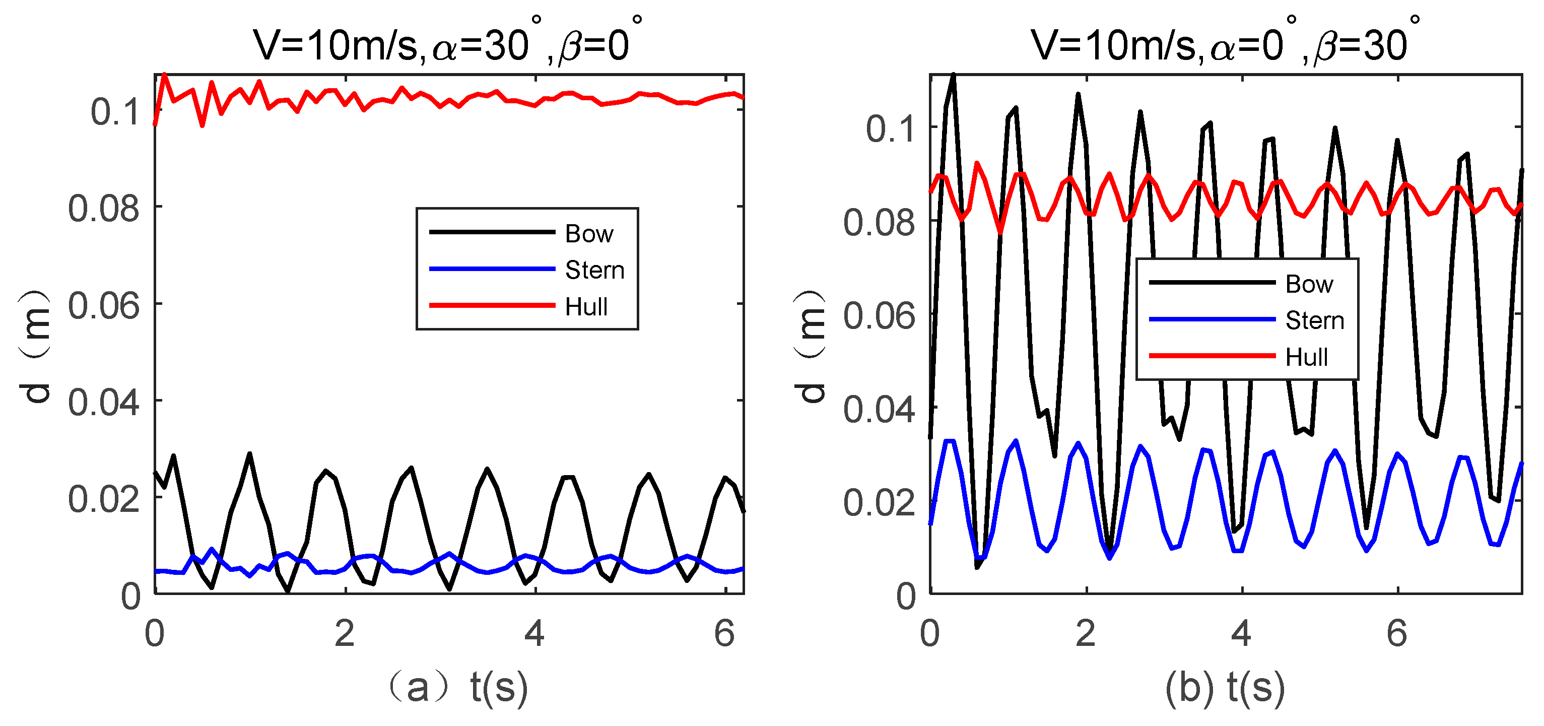
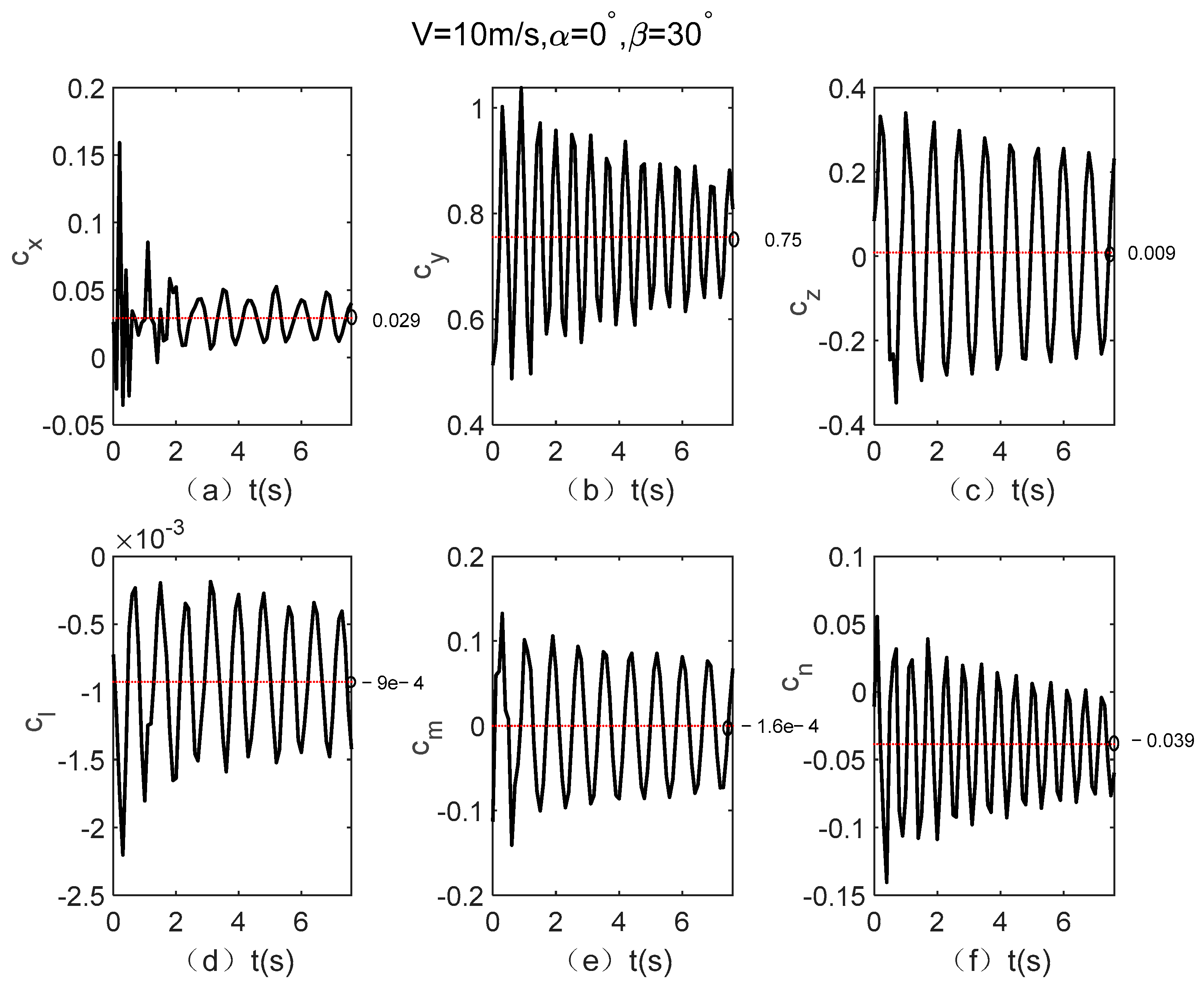
Three monitoring points are selected at key locations on the airship: the nose, the tail, and the section of maximum hull diameter. The structural deformation and aerodynamic response during the FSI-based dynamic analysis are presented in Figure 4 and Figure 5, respectively, where d denotes the magnitude of structural deformation. Here $c_x, c_y, c_z$ represent the aerodynamic force coefficients in the body-fixed x-, y-, z-directions, and $c_l, c_m, c_n$ represent the aerodynamic moment coefficients about the body-fixed x, y, z axes, and α is the angle of attack, β is the sideslip angle.

The fluid–structure interaction process converges gradually, and its steady-state response represents the solution to the coupled FSI equations. To reduce computational cost, when the system exhibits steadily decaying transient oscillatory response at a given angle of attack, the solution is taken as the time-averaged value over one full oscillation period, as shown in Figure 5. However, it should be noted that this time-averaging procedure inherently filters out the transient oscillatory components and aerodynamic damping information.

As shown in Figure 4 and Figure 5, the deformation state of the airship varies under different operating conditions, leading to different aerodynamic forces. For each flight condition, steady-state aerodynamic coefficients are extracted once convergence is achieved. To span the entire flight envelope, interpolation techniques are applied to these discrete data points, enabling a continuous and accurate representation of the aerodynamic characteristics across the operational range [6,25].

2.4. Thrust Model with Deformation

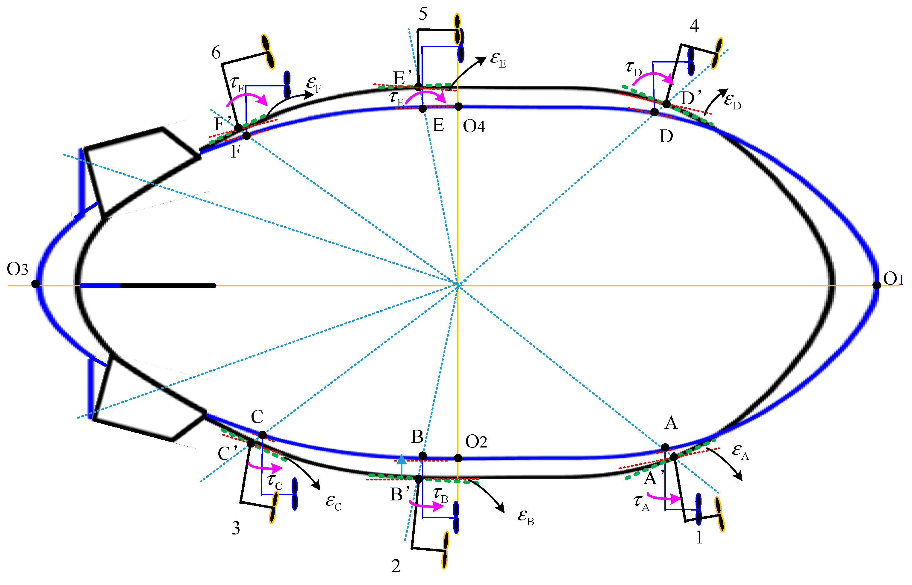
This study does not resolve fine-scale material behaviors—such as wrinkling or localized stretching of the envelope—but instead focuses on global elastic deformations of the entire airship induced by external aerodynamic and control forces. Taking a representative global deformation—uniform expansion—as an example, we neglect the local elasticity of the envelope skin, assuming that both the volume and the centroid of the airship remain unchanged before and after deformation. Additionally, the suspended gondola at the bottom is fixed at its four corners. These constraints enable the isolation and examination of purely elastic effects, decoupled from rigid-body motion. Figure 6 illustrates the airship geometry before and after deformation: the blue curve represents the undeformed shape, while the black curve shows the deformed configuration. Figure 7 further depicts how the airship’s expansion alters the installation orientation of the propellers. The red and green dashed lines indicate the propeller installation planes in the undeformed and deformed states, respectively. The relative angular displacement between these two planes quantifies the change in propeller installation angle. Assuming the propellers maintain a fixed orientation relative to their local installation plane, the deformation results in a net deflection of the installation plane by an angle $\epsilon$ with respect to its original position.

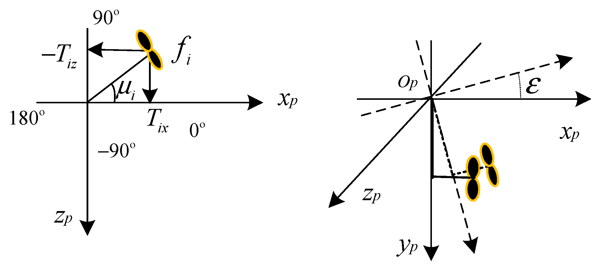
For a rigid airship, each vectored propeller can independently adjust both its thrust magnitude and direction, as shown in Figure 7a. Therefore, there are twelve control variables associated with the vectored propellers $U_{\mathrm{T}}={\left[f_1,f_2,f_3,f_4,f_5,f_6,{\mu }_1,{\mu }_2,{\mu }_3,{\mu }_4,{\mu }_5,{\mu }_6\right]}^{\mathrm{T}}$, and each propeller is decoupled into two vertical components in the x_bo_bz_b plane of the body-fixed frame.

$$\begin{array}{l}{T}_{ix}=f_i\cos {\mu }_i\\ T_{iz}=-f_i\sin {\mu }_i\end{array}$$

(3)

Here the indirect control force $T_{xz}={\left[T_{1x},T_{2x},T_{3x},T_{4x},T_{5x},T_{6x},T_{1z},T_{2z},T_{3z},T_{4z},T_{5z},T_{6z}\right]}^{\mathrm{T}}$ is introduced, which represents the thrust components of the six vectored propellers in the x_bo_bz_b plane, then the control vectored thrust vector $T_{\mathrm{T}}$ can be described as:

$$T_{\mathrm{T}}=P{T}_{\mathrm{xz}}$$

(4)

and the control coefficient matrix $P$ is a constant matrix about mounting positions of propellers.

$$P={\left[\begin{array}{cccccccccccc}1& 1& 1& 1& 1& 1& 0& 0& 0& 0& 0& 0\\ 0& 0& 0& 0& 0& 0& 0& 0& 0& 0& 0& 0\\ 0& 0& 0& 0& 0& 0& 1& 1& 1& 1& 1& 1\\ 0& 0& 0& 0& 0& 0& {\mathrm{y}}_1& {\mathrm{y}}_2& {\mathrm{y}}_3& {\mathrm{y}}_4& {\mathrm{y}}_5& {\mathrm{y}}_6\\ {\mathrm{z}}_1& {\mathrm{z}}_2& {\mathrm{z}}_3& {\mathrm{z}}_4& {\mathrm{z}}_5& {\mathrm{z}}_6& {-\mathrm{x}}_1& {-\mathrm{x}}_2& {-\mathrm{x}}_3& {-\mathrm{x}}_4& {-\mathrm{x}}_5& {-\mathrm{x}}_6\\ {-\mathrm{y}}_1& {-\mathrm{y}}_2& {-\mathrm{y}}_3& {-\mathrm{y}}_4& {-\mathrm{y}}_5& {-\mathrm{y}}_6& 0& 0& 0& 0& 0& 0\end{array}\right]}_{6\times 12}$$

Deformation causes a change in the direction of the propeller thrust, as shown in Figure 7b. In this case, the local thrust coordinate system rotates around the z_p-axis by an angle $\epsilon$ (which can be positive or negative), resulting in a new thrust component.

$$\left[\begin{array}{c}{T}_{ix}^{\prime }\\ T_{iy}^{\prime }\\ T_{iz}^{\prime }\end{array}\right]=R(\epsilon )\left[\begin{array}{c}{T}_{ix}\\ 0\\ T_{iz}\end{array}\right]$$

(5)

where $R=\left[\begin{array}{ccc}\cos \epsilon & -\sin \epsilon & 0\\ \sin \epsilon & \cos \epsilon & 0\\ 0& 0& 1\end{array}\right]$.

For a single propeller, deformation leads to forces in the y_b-direction. If the control commands for pairs of propellers 1 and 4, 2 and 5, 3 and 6 are identical, the additional forces in the y_b-direction generated by deformation can cancel each other out. Therefore, these forces $T_{iy}^{\prime }$ can be ignored. The static weight of the propellers is neglected, as it introduces only a constant bias that does not influence the dynamic servo-elastic coupling under investigation. The deformation does not affect the force in the z_b-direction, while the force in the x_b-direction decreases by a certain factor. This reduction factor can be expressed as $T_{ix}\cos \epsilon$. The error caused by the propeller thrust deflection can be considered equivalent to an efficiency loss, denoted as $\mathrm{\Delta }$; then, we have

$$T_{xz}^{\prime }=\mathrm{\Delta }{T}_{\mathrm{xz}}$$

(6)

where $\mathrm{\Delta }={\left[\begin{array}{cc}\cos {\epsilon }_{\mathrm{T}}\cdot E(6,6)& Z(6,6)\\ Z(6,6)& E(6,6)\end{array}\right]}_{12\times 12}$ and $Z(p,q)$ is an m × n zero matrix, $E(\mathit{n},\mathit{n})$ is the n-dimensional identity matrix.

The positional deviation alters the indirect distribution matrix as $P\prime$. Therefore, the thrust model considering the servo-elasticity can be expressed as:

$$T_T^{\prime }=P\prime T_{xz}^{\prime }=P\prime \mathrm{\Delta }{T}_{\mathrm{xz}}$$

(7)

where $T_{xz}^{\prime }={{\left[T_{1\mathrm{x}}^{\prime },T_{2\mathrm{x}}^{\prime },T_{3\mathrm{x}}^{\prime },T_{4x}^{\prime },T_{5x}^{\prime },T_{6x}^{\prime },T_{1\mathrm{z}}^{\prime },T_{2\mathrm{z}}^{\prime },T_{3\mathrm{z}}^{\prime },T_{4z}^{\prime },T_{5\mathrm{z}}^{\prime },T_{6\mathrm{z}}^{\prime }\right]}^{\mathrm{T}}}_{12\times 1}$,

$$P^{\prime }={\left[\begin{array}{cccccccccccc}1& 1& 1& 1& 1& 1& 0& 0& 0& 0& 0& 0\\ 0& 0& 0& 0& 0& 0& 0& 0& 0& 0& 0& 0\\ 0& 0& 0& 0& 0& 0& 1& 1& 1& 1& 1& 1\\ 0& 0& 0& 0& 0& 0& {\mathrm{y}}_1^{\prime }& {\mathrm{y}}_2^{\prime }& {\mathrm{y}}_3^{\prime }& {\mathrm{y}}_4^{\prime }& {\mathrm{y}}_5^{\prime }& {\mathrm{y}}_6^{\prime }\\ {\mathrm{z}}_1^{\prime }& {\mathrm{z}}_2^{\prime }& {\mathrm{z}}_3^{\prime }& {\mathrm{z}}_4^{\prime }& {\mathrm{z}}_5^{\prime }& {\mathrm{z}}_6^{\prime }& -{\mathrm{x}}_1^{\prime }& -{\mathrm{x}}_2^{\prime }& -{\mathrm{x}}_3^{\prime }& -{\mathrm{x}}_4^{\prime }& -{\mathrm{x}}_5^{\prime }& -{\mathrm{x}}_6^{\prime }\\ -{\mathrm{y}}_1^{\prime }& -{\mathrm{y}}_2^{\prime }& -{\mathrm{y}}_3^{\prime }& -{\mathrm{y}}_4^{\prime }& -{\mathrm{y}}_5^{\prime }& -{\mathrm{y}}_6^{\prime }& 0& 0& 0& 0& 0& 0\end{array}\right]}_{6\times 12}$$

and $T_T^{\prime }={[F_{Tx}^{\prime },F_{Ty}^{\prime },F_{Tz}^{\prime },F_{T\varphi }^{\prime },F_{T\theta }^{\prime },F_{T\psi }^{\prime }]}^{\mathrm{T}}$.

To clearly demonstrate how envelope deformation alters the vectoring propeller mounting positions (Figure 6), we consider a representative global deformation mode, uniform radial expansion. In this specific illustrative example, a constant volume assumption is temporarily introduced to simplify the analytical discussion. It should be noted that this simplification is exclusive to this qualitative analysis; the general FSI framework presented in Section 2.2 and Section 2.3 does not impose this constraint.

2.5. Integrated FSI–Flight Dynamics Model

To establish a unified fluid–structure interaction dynamic model, the equations of motion for a flexible vehicle are derived from the kinetic and potential energies using Lagrange’s equations, expressed in terms of state variables and generalized variables [9]:

$$\left[\begin{array}{ccc}{M}_{11}& M_{12}& M_{13}\\ M_{21}& M_{22}& M_{23}\\ M_{31}& M_{32}& M_{33}\end{array}\right]\left[\begin{array}{c}{\dot{v}}_0\\ \dot{\Omega }\\ \ddot{q}\end{array}\right]=-\left[\begin{array}{c}0\\ 0\\ S_E\end{array}\right]+\left[\begin{array}{c}{f}_I\\ M_I\\ Q_I\end{array}\right]+\left[\begin{array}{c}{f}_G\\ M_G\\ Q_G\end{array}\right]+\left[\begin{array}{c}{f}_{AS}\\ M_{AS}\\ Q_{AS}\end{array}\right]+\left[\begin{array}{c}{f}_{AD}\\ M_{AD}\\ Q_{AD}\end{array}\right]+\left[\begin{array}{c}{f}_{\delta }\\ M_{\delta }\\ Q_{\delta }\end{array}\right]+\left[\begin{array}{c}{f}_{\mathrm{T}}\\ M_{\mathrm{T}}\\ Q_{\mathrm{T}}\end{array}\right]$$

(8)

where $M_{sys}=\left[\begin{array}{ccc}{M}_{11}& M_{12}& M_{13}\\ M_{21}& M_{22}& M_{23}\\ M_{31}& M_{32}& M_{33}\end{array}\right]$ is the mass matrix; ${\dot{v}}_0={\left[\begin{array}{ccc}\dot{u}& \dot{v}& \dot{w}\end{array}\right]}^{\mathrm{T}}$ denote the linear accelerations; $\dot{\Omega }={\left[\begin{array}{ccc}\dot{p}& \dot{q}& \dot{r}\end{array}\right]}^{\mathrm{T}}$ denote the angular accelerations; $\ddot{q}$ is the acceleration of generalized variables decomposed into the body frame, and its dimension is determined by the order of the considered modes; and the right-hand side of the equation denotes external forces, including the internal elastic force $F_{\mathrm{S}}={\left[\begin{array}{ccc}0& 0& -S_E\end{array}\right]}^{\mathrm{T}}$; the term $S_E$ accounts for internal elastic restoring forces due to hull deformation and is retained to ensure dynamic consistency in the coupled flexible-body formulation. While all other forces are conventional external forces—such as the Coriolis force $F_I={\left[\begin{array}{ccc}{f}_I& M_I& Q_I\end{array}\right]}^{\mathrm{T}}$, the gravity $F_G={\left[\begin{array}{ccc}{f}_G& M_G& Q_G\end{array}\right]}^{\mathrm{T}}$, the buoyancy $F_{AS}={\left[\begin{array}{ccc}{f}_{AS}& M_{AS}& Q_{AS}\end{array}\right]}^{\mathrm{T}}$, the aerodynamic control force $F_{AD}={\left[\begin{array}{ccc}{f}_{AD}& M_{AD}& Q_{AD}\end{array}\right]}^{\mathrm{T}}$, the control surface force $F_{\delta }={\left[\begin{array}{ccc}{f}_{\delta }& M_{\delta }& Q_{\delta }\end{array}\right]}^{\mathrm{T}}$, and the multiple propeller force $F_{\mathrm{T}}={\left[\begin{array}{ccc}{f}_{\mathrm{T}}& M_{\mathrm{T}}& Q_{\mathrm{T}}\end{array}\right]}^{\mathrm{T}}$. Each term includes the external forces f, the moments M and the generalized elastic force Q. These external elastic forces are decomposed into the body frame, as the generalized variables are expressed in the body frame.

According to Lagrange’s equations, for given external forces, the moment generated is related to elastic deformation, and the elastic forces are related to the mode shapes. The decoupled deformation at node i is given by:

$$d_i={\overline{\Phi }}_i{q}^{\prime }$$

(9)

where $q^{\prime }={\left.{\left[q_{1x},q_{2x},\dots ,q_{jx},q_{1y},q_{2y},\dots ,q_{jy},q_{1z},q_{2z},\dots ,q_{jz}\right]}^{\mathrm{T}}\right|}_{3j\times 1}$ and matrix of deformations of node i is:

$${\overline{\Phi }}_i={\left[\begin{array}{ccc}{\zeta }_{1i},{\zeta }_{2i},\dots ,{\zeta }_{ji}& Z(1,j)& Z(1,j)\\ Z(1,j)& {\zeta }_{1i},{\zeta }_{2i},\dots ,{\zeta }_{ji}& Z(1,j)\\ Z(1,j)& Z(1,j)& {\zeta }_{1i},{\zeta }_{2i},\dots ,{\zeta }_{ji}\end{array}\right]}_{3\times 3j}$$

(10)

Unlike the classical formulation in Equation (1) where mode shapes are decomposed into Cartesian components scaled by a single scalar q, Equation (10) retains the mode shape as an undecomposed vector ${\zeta }_{ji}$. To capture direction-dependent dynamic responses, the generalized coordinates are defined as a vector of independent variables $q_j^{\prime }={\left[q_{jx},q_{jy},q_{jz}\right]}^{\mathrm{T}}$. This allows the deformation amplitudes along the x_b, y_b, and z_b axes to evolve independently despite sharing the same spatial basis, thereby relaxing the fixed-ratio constraint inherent in standard modal superposition.

For servo-elastic control, the vibration modes ${\Phi }_{\delta }$,${\Phi }_{\mathrm{T}}$ and the deformations $d_{\mathrm{\delta }}$, $d_{\mathrm{T}}$ at the nodes of thrust installation points and the control surface action points will be the primary focus. The control force from the surface is derived from:

$$F_{\delta }={\left[\begin{array}{c}E(3,3)\\ {r_{\mathrm{\delta }}}^{\times }+{d_{\mathrm{\delta }}}^{\times }\\ {\overline{\Phi }}_{\delta }^{\mathrm{T}}\end{array}\right]}_{(6+3j)\times 3}{f}_{\mathrm{\delta }}$$

(11)

where $f_{\delta }={[q_{\infty }{S}_{ref}{c}_{x_{{\delta }_a}}{\delta }_a,q_{\infty }{S}_{ref}{c}_{y_{{\delta }_r}}{\delta }_r,q_{\infty }{S}_{ref}{c}_{z_{{\delta }_e}}{\delta }_e]}^{\mathrm{T}}$, $M_{\delta }=\left(r_{\mathrm{\delta }}^{\times }+d_{\mathrm{\delta }}^{\times }\right)f_{\mathrm{\delta }}$ and $Q_{\delta }={\overline{\Phi }}_{\delta }^{\mathrm{T}}{f}_{\delta }$, and $q_{\infty }=1/2\rho V^2$ is the dynamic pressure of airflow, $S_{ref}=Vo{l}^{2/3}$ is the reference surface and $l_{ref}=Vo{l}^{1/3}$ is the reference length ($Vol$: airship volume). $c_{x_{{\delta }_a}}$, $c_{y_{{\delta }_r}}$ and $c_{z_{{\delta }_e}}$ are the aerodynamic force coefficients of the control surfaces. ${\delta }_a$, ${\delta }_e$ and ${\delta }_r$ are deflection angles of the aerodynamic control surfaces.

• Here $d^{\times }$ is the cross product of vector $d$, $d^{\times }=\left[\begin{array}{ccc}0& -d_z& d_y\\ d_z& 0& -d_x\\ -d_y& d_x& 0\end{array}\right]$, and $d_{\mathrm{\delta }}$ is the deformation at the control surface mounting point.

The control force generated by the propellers is derived from:

$$F_{\mathrm{T}}^{\prime }={\left[\begin{array}{c}E(3,3)\\ {r_{\mathrm{T}}}^{\times }+{d_{\mathrm{T}}}^{\times }\\ {\overline{\Phi }}_{\mathrm{T}}^{\mathrm{T}}\end{array}\right]}_{(6+3j)\times 3}{f}_{\mathrm{T}}$$

(12)

where $f_{\mathrm{T}}=\cos \epsilon {\left[T_{1x},T_{2x},T_{3x},T_{4x},T_{5x},T_{6x}\right]}^{\mathrm{T}}$, $M_{\mathrm{T}}=\left({r_{\mathrm{T}}}^{\times }+{d_{\mathrm{T}}}^{\times }\right)f_{\mathrm{T}}$ and $Q_{\mathrm{T}}={\overline{\Phi }}_{\mathrm{T}}^{\mathrm{T}}{f}_{\mathrm{T}}$, and $d_{\mathrm{T}}$ represents the deformation at the thrust mounting point. The dynamic response is obtained through the numerical integration of Equation (8). Specifically, Equation (8) was numerically integrated using MATLAB’s ode45 solver, which employs an explicit variable-step Runge–Kutta (4,5) method. Through convergence analysis, a fixed output sampling time of Ts = 0.01 s was determined to be sufficient to prevent numerical divergence and capture the high-frequency dynamics of the flexible airship.

It is important to clarify that the uniform expansion mode discussed in Section 2.4 is presented solely as an illustrative example to demonstrate the modeling procedure and the physical interpretation of the coupling terms. The developed FSI framework, however, is formulated based on a general modal representation and is fully applicable to arbitrary deformation modes, including the non-axisymmetric shapes depicted in Figure 2. Consequently, the subsequent analysis and control design utilize this general formulation without restriction to specific mode shapes.

3. Servo-Elastic Control System Design

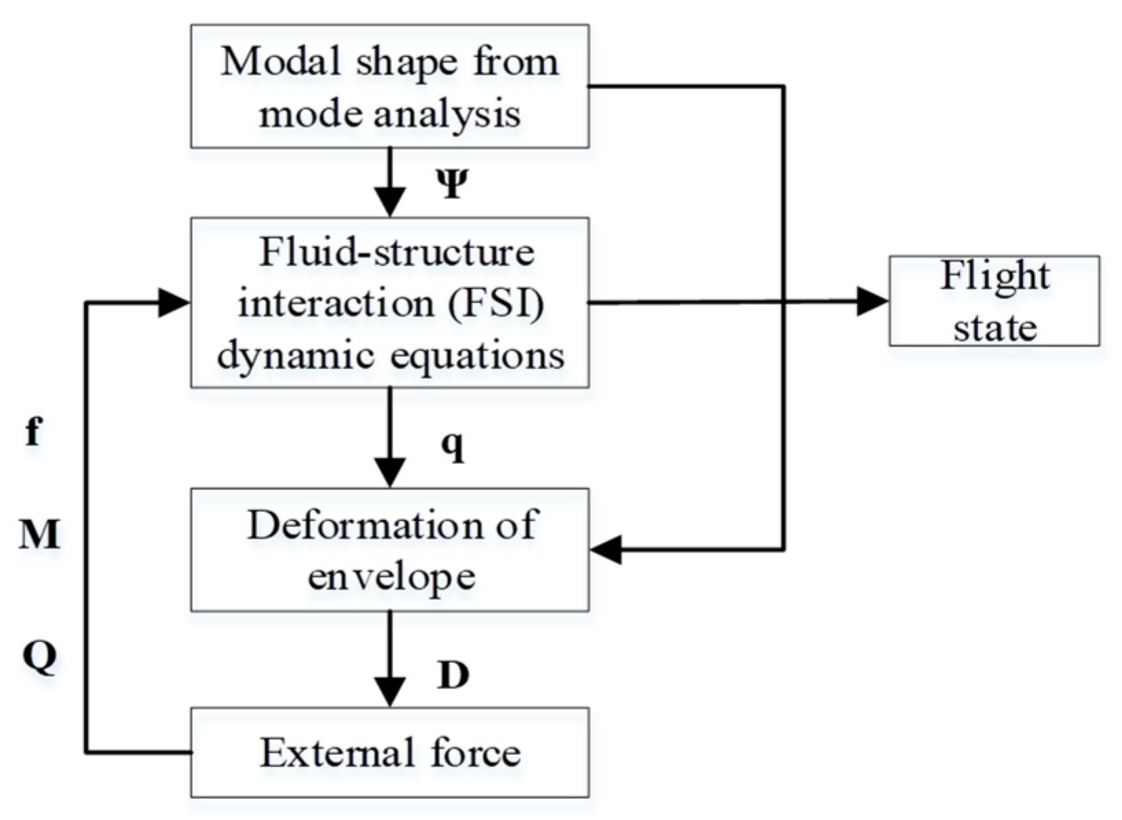
In theory, deformation data at the installation points can be obtained based on a fluid–structure interaction model, as shown in Figure 8, and by solving Equation (9). The efficiency loss of the thrust can be modeled separately to account for changes in posture and installation position deviations of the actuators. The difference between the thrust force without deformation and the thrust force with deformation is referred to as the servo-elastic correction. To make the control performance of the airship after elastic deformation similar to that of a rigid airship, a disturbance estimation method is implemented. The servo-elastic correction is incorporated into disturbance compensation for controller design. This approach not only improves control accuracy but also adapts to real-time variations in operating conditions, providing a more reliable solution for practical applications.

3.1. Controller Design

Equation (8) can be expressed in world frame in a compact form,

$$M_{\mathrm{sys}}J\ddot{X}=F_{\mathrm{S}}+F_{\mathrm{I}}+F_{\mathrm{G}}+F_{\mathrm{AS}}+F_{\mathrm{A}}+F_{\mathrm{T}}+F_{\mathrm{\delta }}$$

(13)

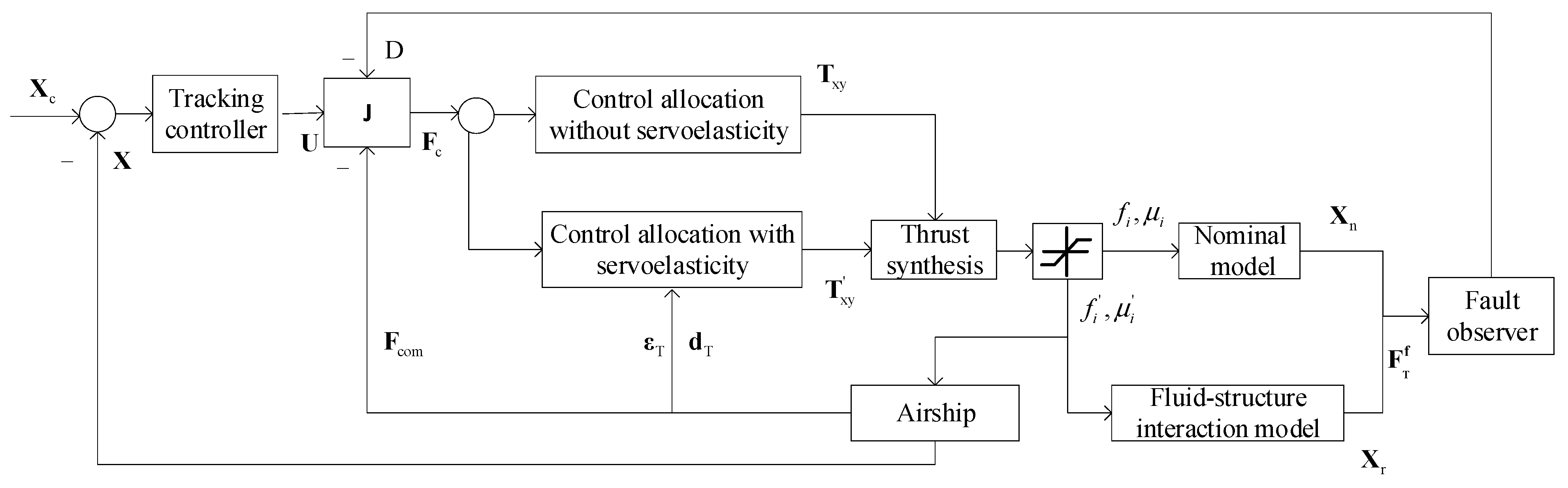
where $X={\left[x,y,z,\varphi ,\theta ,\psi ,q_{1x},q_{2x},\dots ,q_{jx},q_{1y},q_{2y},\dots ,q_{jy},q_{1z},q_{2z},\dots ,q_{jz}\right]}^{\mathrm{T}}$ is the state of the fluid–structure interaction model in the inertial coordinate system, and the transformation matrix is $J=\left[\begin{array}{ccc}{R}_{\mathrm{BI}}& Z(3,3)& Z(3,3j)\\ Z(3,3)& E(3,3)& Z(3,3j)\\ Z(3j,3)& Z(3j,3)& E(3j,3j)\end{array}\right]$, where $R_{\mathrm{BI}}$ is the direction cosine matrix. Although aerodynamic control surfaces are generally considered as control variables, their maneuvering capability is weak at low speeds. This weakness can lead to saturation and induce uncontrolled attitude changes. Therefore, in this paper, the control surfaces are kept in a neutral position and are not involved in the control, $F_{\mathrm{\delta }}=0$. Figure 9 shows the general structure of the control system. The total control force consists of PD feedback, feedforward compensation, and disturbance estimation compensation. The feedforward compensation force is given by $F_{\mathrm{com}}=F_{\mathrm{S}}+F_{\mathrm{I}}+F_{\mathrm{G}}+F_{\mathrm{AS}}+F_{\mathrm{A}}$. The change in the thrust force caused by elastic deformation are estimated by a disturbance compensator D, which is designed in the next section.

Given the tracking error $X_{\mathrm{e}}(t)=X_{\mathrm{c}}-X$, a PD tracking controller is designed as

$$U=M_{\mathrm{sys}}J({\ddot{X}}_{\mathrm{c}}+K_{\mathrm{P}}{X}_{\mathrm{e}}+K_{\mathrm{D}}{\dot{X}}_{\mathrm{e}})$$

(14)

Then, the total control force is given by,

$$F_{\mathrm{c}}=M_{\mathrm{sys}}J({\ddot{X}}_{\mathrm{c}}+K_{\mathrm{P}}{X}_{\mathrm{e}}+K_{\mathrm{D}}{\dot{X}}_{\mathrm{e}})-F_{\mathrm{com}}-D$$

(15)

The overall control force $F_{\mathrm{c}}$ is generated by multiple vectored propellers and is directed to two channels: one is the control allocation module that does not consider servo-elasticity, as shown in Equation (16a), and the other is the control allocation module that accounts for servo-elasticity, as shown in Equation (16b).

$$T_{\mathrm{xy}}={\left.\left\{\left[\begin{array}{c}E(6,6)\\ \begin{array}{cc}{\overline{\Phi }}_{\mathrm{T}}^{\mathrm{T}}& Z(3j,3)\end{array}\end{array}\right]P\right\}\right|}_{(6+3j)\times 12}^{+}{F}_{\mathrm{c}}$$

(16a)

$$T_{\mathrm{xy}}^{\prime }={\left\{\left[\begin{array}{c}E(6,6)\\ \begin{array}{cc}{\overline{\Phi }}_{\mathrm{T}}^{\mathrm{T}}& Z(3j,3)\end{array}\end{array}\right]P^{\prime }\mathrm{\Delta }\right\}}_{(6+3j)\times 12}^{+}{F}_{\mathrm{c}}$$

(16b)

Here the term Δ (as derived from Equation (6) under Figure 6 simplification) generally represents the propeller’s attitude deviation across all three axes in practical applications. Then, thrust synthesis involves decomposing the 12-dimensional indirect control forces $T_{\mathrm{xy}}$ or $T_{\mathrm{xy}}^{\prime }$ into the force magnitudes and deflection angles of six individual propellers, similar to:

$$\begin{array}{l}{f}_i=\sqrt{T_{ix}^2+T_{iz}^2}\\ {\mu }_{\mathrm{i}}={\tan }^{-1}(T_{ix}/-T_{iz})\end{array}$$

(17)

The actual numerical computations of ${\mu }_i$ are implemented in MATLAB R2024b using atan2, ensuring correct quadrant resolution during simulation. For real control variables $f_i^{\prime }$, ${\mu }_i^{\prime }$ is different from $f_i$, ${\mu }_i$ due to the consideration of servo-elasticity. A saturation model is then used to limit the maximum output force of each propeller, as $0\le f_i\le 500 \mathrm{N}, -180°\le {\mu }_i\le 180°, i=1,\dots ,6$. The actual force acting on the airship, according to the thrust model (Equation (7)), $F_{\mathrm{cr}}$ is given by:

$$F_{\mathrm{cr}}={\left[\begin{array}{c}E(6,6)\\ \begin{array}{cc}{\overline{\Phi }}_{\mathrm{T}}^{\mathrm{T}}& Z(3j,3)\end{array}\end{array}\right]}_{(6+3j)\times 6}{P}^{\prime }\mathrm{\Delta }{T}_{\mathrm{xy}}^{″}$$

(18)

where $T_{\mathrm{xy}}^{″}$ is the indirect control force after the saturation module. While the proposed theoretical framework is general and capable of handling arbitrary mode shapes and axes, the specific numerical analysis presented herein focuses on the first and second-order bending modes using the simplified deflection model Δ derived in Figure 7. Although these modes are not axially symmetric, this simplification serves as a representative case study to isolate and highlight the primary servo-elastic coupling effects.

3.2. Disturbance Estimation

The nominal system without servo-elasticity $M_{\mathrm{sys}}J{\dot{X}}_{\mathrm{n}}=F_{\mathrm{com}}+F_{\mathrm{T}}$ and the real system with servo-elasticity $M_{\mathrm{sys}}J\dot{X}=F_{\mathrm{com}}+F_{\mathrm{T}}^{\prime }$ are considered. The difference in thrust caused by elastic deformation, compared to the thrust in the nominal model, is referred to as the thrust fault.

$$F_{\mathrm{T}}^{\mathrm{f}}=F_T^{\prime }-F_T=M_{\mathrm{sys}}(\dot{X}-{\dot{X}}_{\mathrm{n}})$$

(19)

To compensate the difference in real force with the nominal control force, the linear estimator is used to estimate the faulty forces $F_T^f$ caused by various factors [26].

$$\left\{\begin{array}{l}{\dot{D}}_{\mathrm{f}}=-\Lambda D_{\mathrm{f}}+\Lambda F_T^{\mathrm{f}}\\ F_T^{\mathrm{f}}=M_{\mathrm{sys}}J\ddot{X}-M_{\mathrm{sys}}J{\ddot{X}}_{\mathrm{n}}\end{array}\right.$$

(20)

Due to the large volume and high inertia of the airship, its rigid-body dynamics evolve on a much slower time scale than the high-frequency servo-elastic modes. Consequently, the thrust variations caused by servo-elasticity can be considered as quasi-static, allowing their dynamic time derivatives to be neglected in the flight dynamics equations.

Therefore ${\dot{F}}_T^{\mathrm{f}}=0$ and $D_{\mathrm{f}}$ is the estimated values of the fault control force. The fault estimation error can be defined as: $e=D_{\mathrm{f}}-F_T^{\mathrm{f}}$, then

$$\dot{e}={\dot{D}}_{\mathrm{f}}-{\dot{F}}_T^{\mathrm{f}}=-\Lambda D_{\mathrm{f}}+\Lambda F_T^{\mathrm{f}}=-\Lambda e$$

(21)

$$X\to X_{\mathrm{n}}$$

where $\Lambda$ is a diagonal coefficient matrix with all positive elements. Thus, the Hurwitz condition of error Equation (21) is satisfied; then the error of fault estimation approaches zero, and the real fault force is accurately estimated as follows:

$$D_{\mathrm{f}}\to F_T^f$$

(22)

4. Simulation Results

4.1. Open-Loop Response Analysis

To simplify the problem, we will neglect the effects of axial deformations and ignore the local breathing modes. Instead, we will focus on the impacts of the first- and second-order beam bending modes in the global vibration modes for the servo-elastic control analysis. The expressions for the first two dominant mode shapes are ${\Phi }_{\mathrm{i}}=\left[\begin{array}{cc}0& 0\\ {\zeta }_{1iy}& {\zeta }_{2iy}\\ {\zeta }_{1iz}& {\zeta }_{2iz}\end{array}\right]$. Here ${\zeta }_{1iy}$, ${\zeta }_{1iz}$ and ${\zeta }_{2iy}$, ${\zeta }_{2iz}$ represent the first- and second-order beam bending modes in the x_bo_by_b and x_bo_bz_b planes, respectively. The generalized variables for each degree of freedom are decomposed into the y_b- and z_b-directions in the body-fixed coordinate system as $q_s={\left[\begin{array}{cccc}{q}_{1y}& q_{2y}& q_{1z}& q_{2z}\end{array}\right]}^{\mathrm{T}}$; $q_{jy}, q_{\mathrm{jz}}$ are the j-th generalized variables around the z_b-axis and y_b-axis, respectively. $q_{1y}, q_{1\mathrm{z}}$ represent the lateral and vertical deformation amplitudes associated with the first dominant bending mode, $q_{2y},q_{2\mathrm{z}}$ do the same for the second dominant mode. This decomposition treats the y_b- and z_b -components as if they were independent degrees of freedom, even though they originate from the same underlying mode shapes. The y_b-z_b decomposition is not derived from modal theory but from engineering convenience; no ratio is defined; the four multipliers are treated as independent. While this contradicts the mathematical nature of normal modes, it can be acceptable in quasi-static or open-loop parametric studies where directional deformation effects dominate [9].

This approach establishes decoupled elastic dynamic equations. The decoupled deformation of node i is $d_i={\overline{\Phi }}_i{q}_s$, and ${\overline{\Phi }}_i=\left[\begin{array}{cccc}0& 0& 0& 0\\ {\zeta }_{1i}& {\zeta }_{2i}& 0& 0\\ 0& 0& {\zeta }_{1i}& {\zeta }_{2i}\end{array}\right]$.

As shown in Equation (12), where $Q_{\mathrm{T}}={\overline{\Phi }}_{\mathrm{T}}^{\mathrm{T}}{f}_{\mathrm{T}}$, $Q_{\mathrm{T}}$ is the sum of the elastic forces generated by the six vector propellers at their installation positions ${\mathrm{T}}_i$:

$$Q_{\mathrm{T}}={\overline{\Phi }}_{\mathrm{T}}^{\mathrm{T}}{f}_{\mathrm{T}}={\displaystyle \sum _{i=1}^6\left[\begin{array}{ccc}0& {\zeta }_{1{\mathrm{T}}_i}& 0\\ 0& {\zeta }_{2{\mathrm{T}}_i}& 0\\ 0& 0& {\zeta }_{1{\mathrm{T}}_i}\\ 0& 0& {\zeta }_{2{\mathrm{T}}_i}\end{array}\right]\left[\begin{array}{c}{T}_{ix}\\ 0\\ T_{iz}\end{array}\right]}=\left[\begin{array}{c}0\\ 0\\ {\displaystyle \sum _{i=1}^6{\zeta }_{1{\mathrm{T}}_i}{T}_{i\mathrm{z}}}\\ {\displaystyle \sum _{i=1}^6{\zeta }_{2{\mathrm{T}}_i}{T}_{iz}}\end{array}\right]$$

(23)

where ${\zeta }_{j{\mathrm{T}}_i}$, ${\zeta }_{j{\mathrm{T}}_i}$ $j=1,2, i=1,2,\dots ,6$ represents the j-th order modal shape, occurring at the i-th propeller position. Since the vector thrust cannot generate lateral forces and the elastic deformation in the x_b-axis direction is ignored, the first two rows of the matrix $Q_{\mathrm{T}}$ are zero, indicating that there is no lateral control capability and elastic suppression ability for the generalized variables $q_{1y}, q_{2y}$ around the z_b-axis.

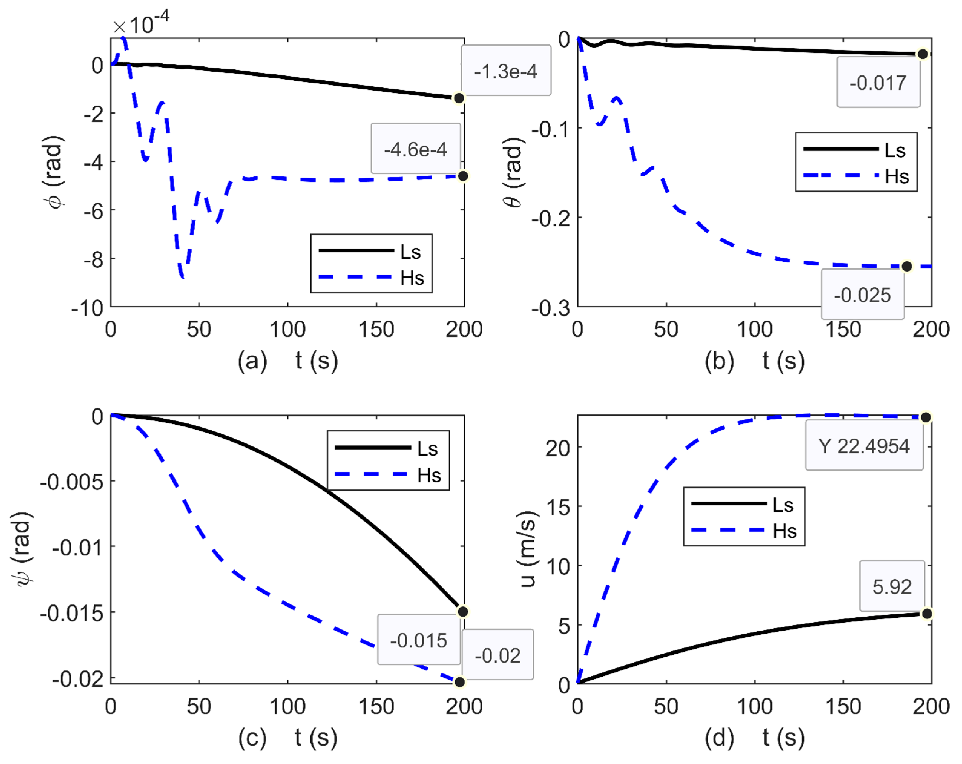
Figure 10 and Figure 11 illustrate the open-loop responses of the servo-elastic model at both high (Hs) and low speeds (Ls). The comparison between high-speed and low-speed cases is presented to demonstrate that the modal response characteristics remain largely consistent across different flight speeds. In open-loop motion, the yaw tends to diverge, although this divergence occurs very slowly, as shown in Figure 11c. Meanwhile, the pitch stabilizes at a new equilibrium point, as illustrated in Figure 11b. It can be observed that there is a strong correlation between yaw and the elastic motion around the z_b-axis, as shown in Figure 10c,d and Figure 11c, as well as between pitch and the elastic motion around the y_b-axis, as shown in Figure 10e,f and Figure 11b.

In the finite element model, the elastic force is the integral of product of the mode shape and the distributed force, as given by the elastic force expression for a given concentrated force in Equation (12). Since the airship’s gravity includes the concentrated mass of the pod and tail, the distribution of gravitational forces differs significantly from the distribution of buoyant forces. This difference leads to errors between the elastic forces due to gravity and those due to buoyancy. Thus, a steady-state deviation is observed in the elastic motion around the y_b-axis, as shown in Figure 10e,f.

4.2. Servo-Elastic Control Simulation Analysis

In this section, the trace tracking and elastic suppression are implemented together to validate the proposed strategies. For a given control target:

$$X_{\mathrm{c}}(t)={\left[\begin{array}{cccccccccc}5+3t& 7+4t& 0& 0& 0& \mathrm{atan}2(4,3)& 0& 0& 0& 0\end{array}\right]}^{\mathrm{T}}$$

where t represents the simulation time.

The paper compares the trajectory tracking results with and without elastic suppression. The controller parameters for trajectory tracking with elastic suppression (SEC) are as follows:

$$K_{\mathrm{P}}=\mathrm{diag}\left(\left[\begin{array}{cccccccccc}0.2& 0.1& 6& 10& 0& 2& 0& 0& 70& 0\end{array}\right]\right)$$

$$K_{\mathrm{D}}=\mathrm{diag}\left(\left[\begin{array}{cccccccccc}4& 2& 1& 4& 0& 20& 0& 0& 5& 0\end{array}\right]\right)$$

The parameter design for trajectory tracking controller (TTC) without elastic suppression is as follows:

$$K_{\mathrm{P}}=\mathrm{diag}\left(\left[\begin{array}{cccccccccc}0.2& 0.1& 6& 10& 0& 2& 0& 0& 0& 0\end{array}\right]\right)$$

$$K_{\mathrm{D}}=\mathrm{diag}\left(\left[\begin{array}{cccccccccc}4& 2& 1& 4& 0& 20& 0& 0& 0& 0\end{array}\right]\right)$$

The gains $K_{\mathrm{P}}$ and $K_{\mathrm{D}}$ were determined through manual tuning based on simulation-based trial and error. Due to the uncontrolled elastic motion $q_{1y},$$q_{2y}$ around the z_b-axis, the elastic motion around the y_b-axis is primarily influenced by first-order generalized variable $q_{1\mathrm{z}}$. To focus on the key issue and reduce the parameter-tuning effort, servo-elastic control is only applied to $q_{1\mathrm{z}}$ channel.

During the parameter tuning process, it was observed that the proportional coeffcient P had already reached a large value, and the effect of the differential coefficient D was negligible. Therefore, only P control is used for this channel. At present, only position tracking and servo-elastic suppression are implemented, while pitch angle control is not included. The reasons for not controlling the pitch angle will be explained in the subsequent simulation results.

The parameter design of the disturbance estimator is as follows:

$$\Lambda =\mathrm{diag}\left(\left[\begin{array}{cccccccccc}1& 1& 1& 1& 1& 1& 1& 1& 1& 1\end{array}\right]\right)$$

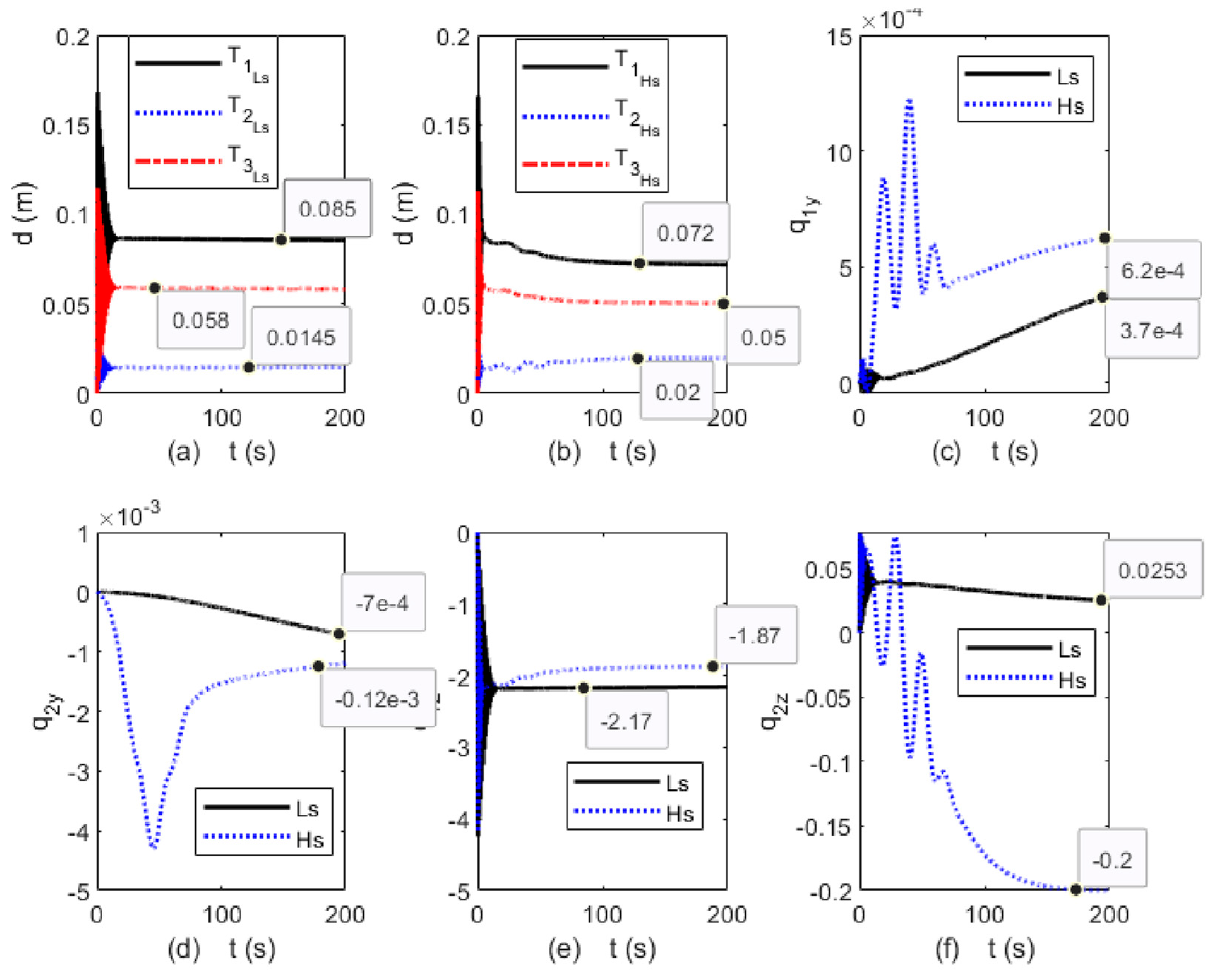
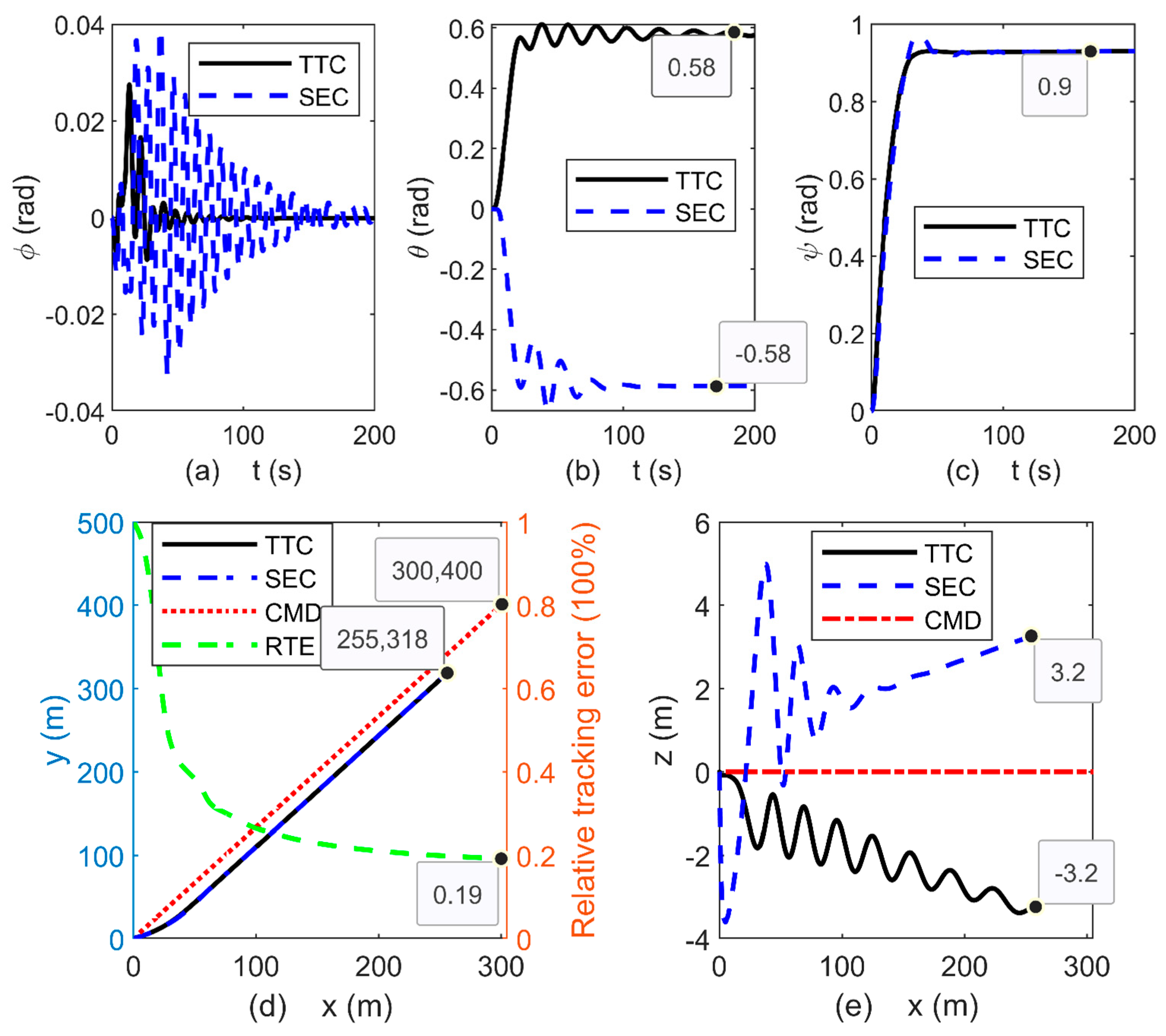
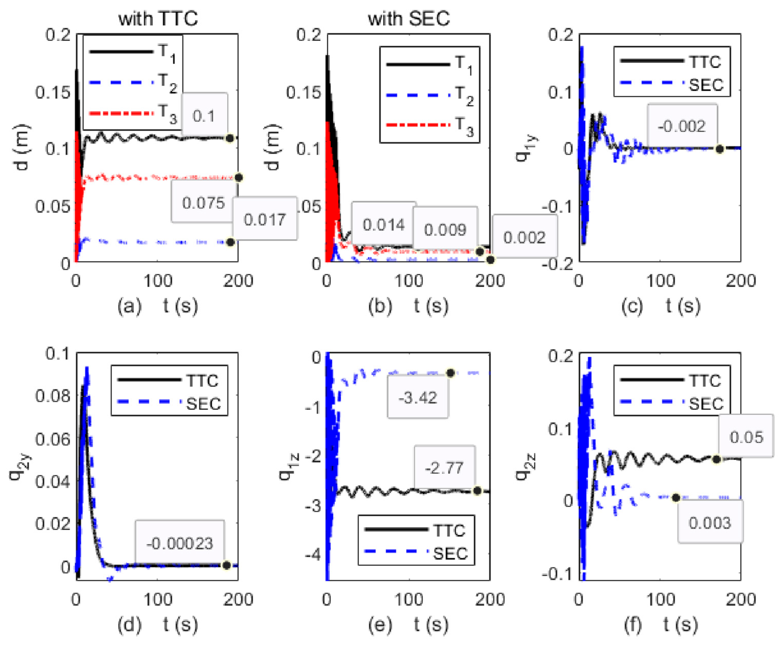
Figure 12 shows the attitude and trajectory tracking results, while Figure 13 presents the displacement of the three sets of propellers and the suppression results of the generalized variables.

In Figure 12 and Figure 13, the markers ‘TTC’ and ‘SEC’ denote simulation results under two control configurations, both with pitch control disabled: ‘TTC’ corresponds to position tracking alone without servo-elastic compensation, while ‘SEC’ includes active suppression of elastic deformation in addition to position tracking. The marker ‘CMD’ represents the ideal trajectory, while T₁, T₂, and T₃ indicate the installation positions of propellers 1, 2, and 3, respectively. Both control strategies achieve satisfactory trajectory tracking performance, improving trajectory tracking accuracy by 19% in terms of RMS position error (RTE) over a 300 s maneuver.

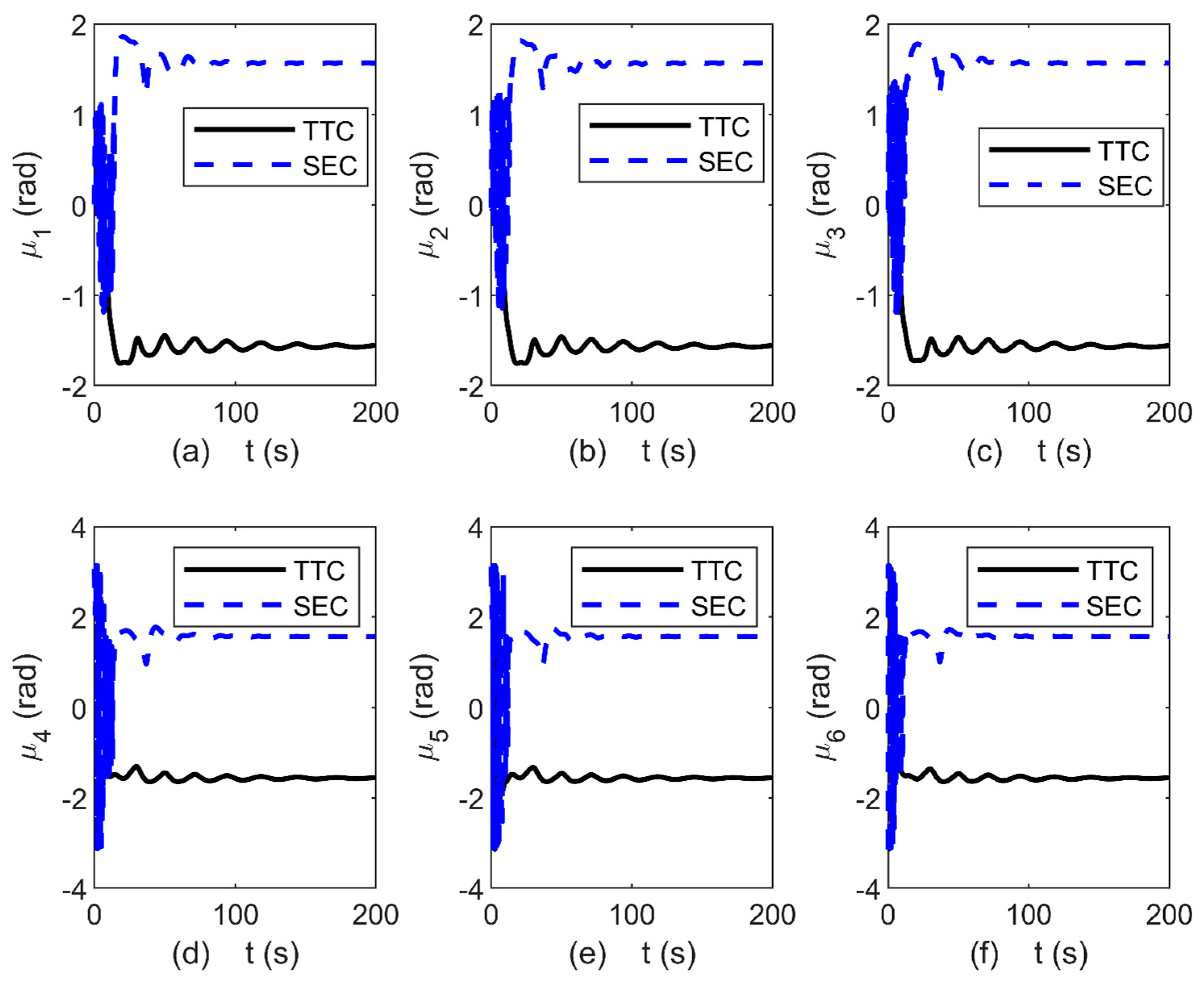
However, since pitch attitude is not actively controlled, the steady-state pitch angle exhibits opposite signs in the without and with servo-elastic compensation, as shown in Figure 12b. This phenomenon arises from changes in force distribution caused by structural deformation and its compensation. As illustrated in Figure 14, the deflection angles of a representative propeller in these two scenarios are oriented in opposite directions. Due to the elastic suppression inherent in SEC, a pitch angle of−0.58 rad is induced, resulting in a change in flight altitude of 3.3 m, as can be seen in Figure 12e.

The blue dashed line represents the results of elastic suppression. Compared to the TTC results, the SEC shows that the generalized variables quickly converge to a smaller equilibrium position, as seen in Figure 13e. This results in a reduction in the deformation at the installation positions of the three sets of propellers to a certain value, as shown in Figure 13b, under SEC case, the deformation at the vectored thrust attachment points is reduced to approximately 10% of the magnitude observed in the TTC case. As seen in Figure 13c,d,f, the other elastic motion stabilizes naturally.

In both cases, the primary effect is a change in the generalized variables $q_{1z}$, $q_{2z}$, as shown in Figure 13e,f. There is a strong coupling between pitch and elasticity. A stable value of $q_{1z}$ and $q_{2z}$ corresponds to a stable pitch angle. During the initial phase, the yaw motion induces changes in $q_{1y}$, $q_{2y}$ around the z_b-axis. As the yaw reaches stability, as shown in Figure 12c, the generalized variables $q_{1y}$, $q_{2y}$ also stabilize, as seen in Figure 13c,d.

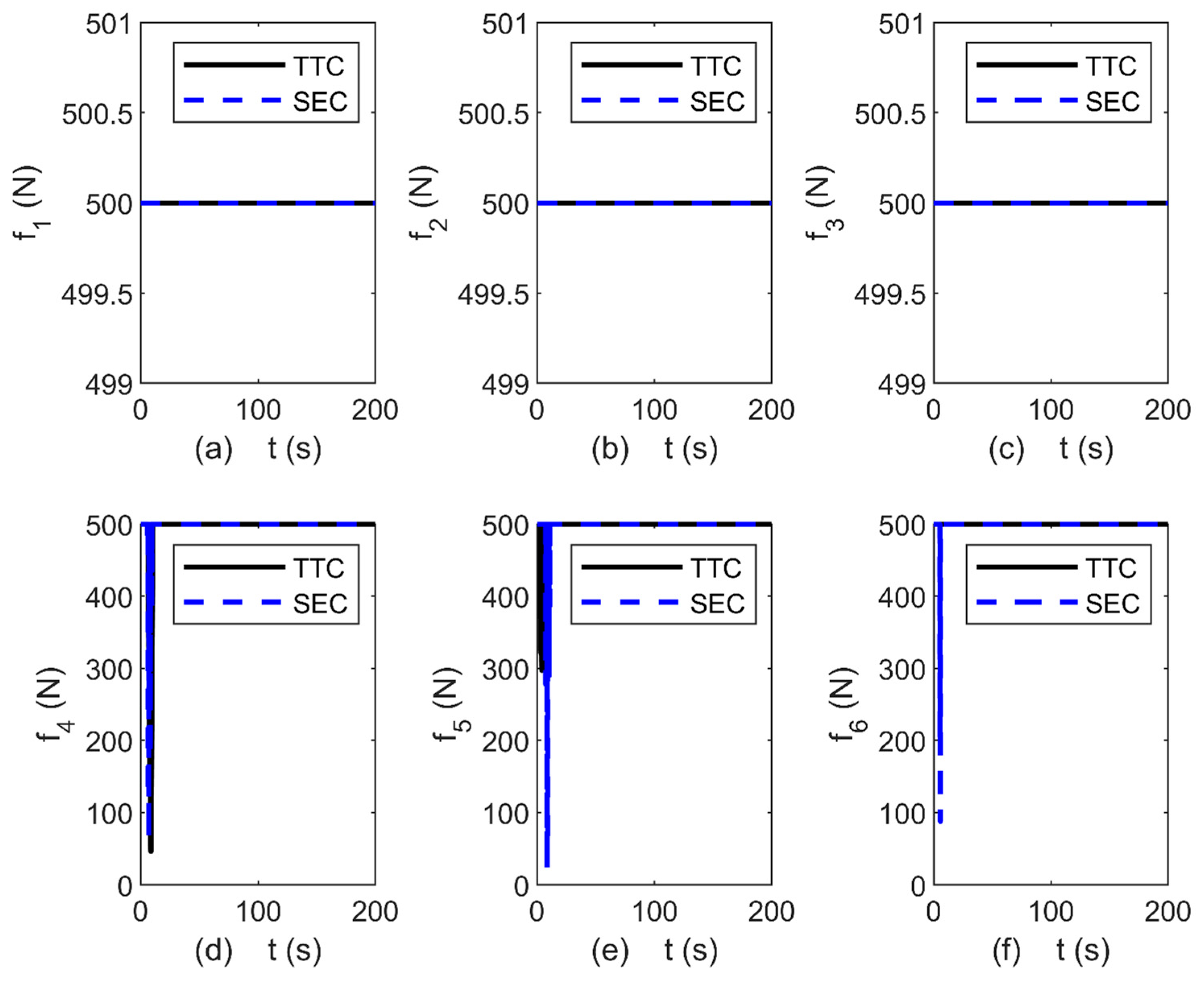
In SEC, the motion of the generalized variables is not completely suppressed in Figure 13e,f, due to thrust saturation, as shown in Figure 15. Both controllers have reached thrust saturation, but the vector angles are having opposite signs, as shown in Figure 14.

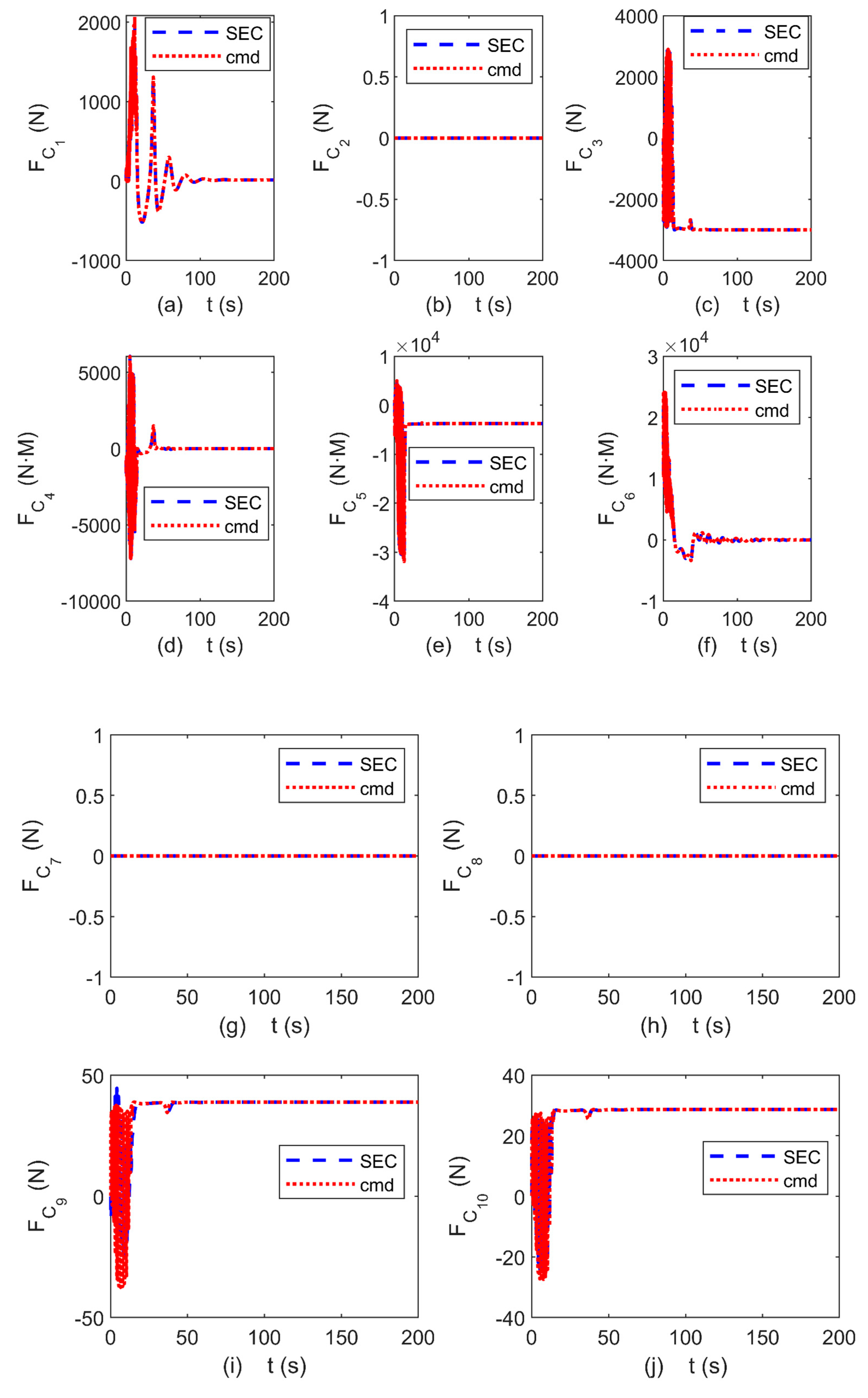
Figure 16 shows the variation in control force for SEC. Here, ‘cmd’ refers to the command control, and ‘SEC’ denotes the real control forces with disturbance compensation. After compensating for the servo-elastic disturbances, the actual control forces (blue line) in all directions closely follow the commanded control forces (red line).

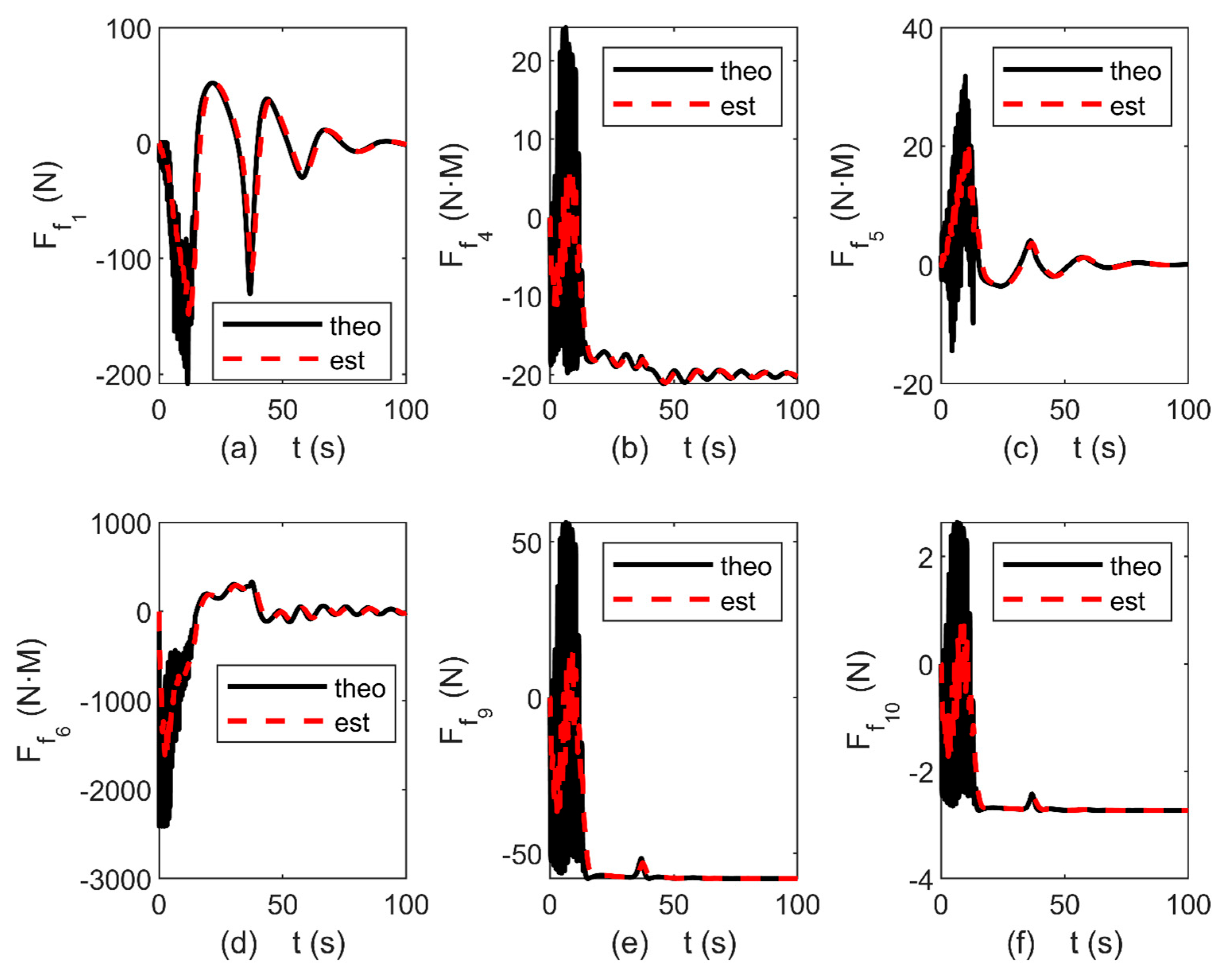
The comparison between the estimated value of the servo-elastic error and the theoretical error value from the disturbance observer is shown in Figure 17. As indicated by Equations (5) and (23), the airship lacks lateral control capability, meaning it cannot control lateral displacement or lateral elastic deformation. Consequently, channels 2, 7, and 8 have no control authority, as demonstrated in Figure 16b,g,h. As shown in Equation (5), since the model does not have servo-elasticity errors in the z_b-axis, the disturbance estimation in the z_b-axis is zero. In Figure 17, ‘theo’ represents the theoretical value of the fault, and ‘est’ represents the estimated value of the fault. The disturbance estimator can effectively estimate the deviation forces caused by servo-elasticity and track changes in the errors. As it is a linear disturbance estimator, assuming the rate of change in the disturbance is zero, there is some deviation in the disturbance estimation accuracy during the initial phase of motion; however, in the later stages, after the motion stabilizes, the disturbance estimator accurately estimates the error caused by the servo-elasticity.

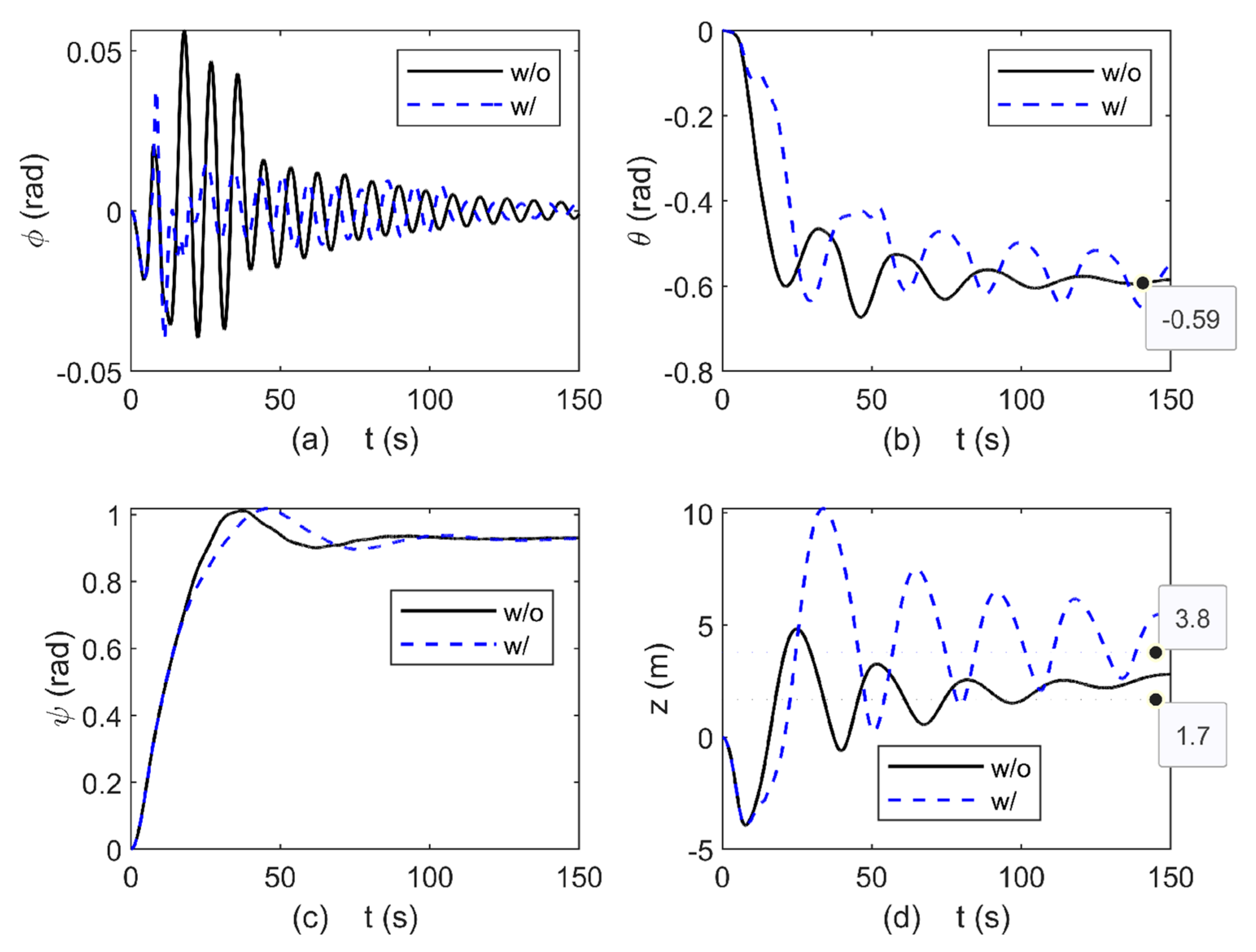
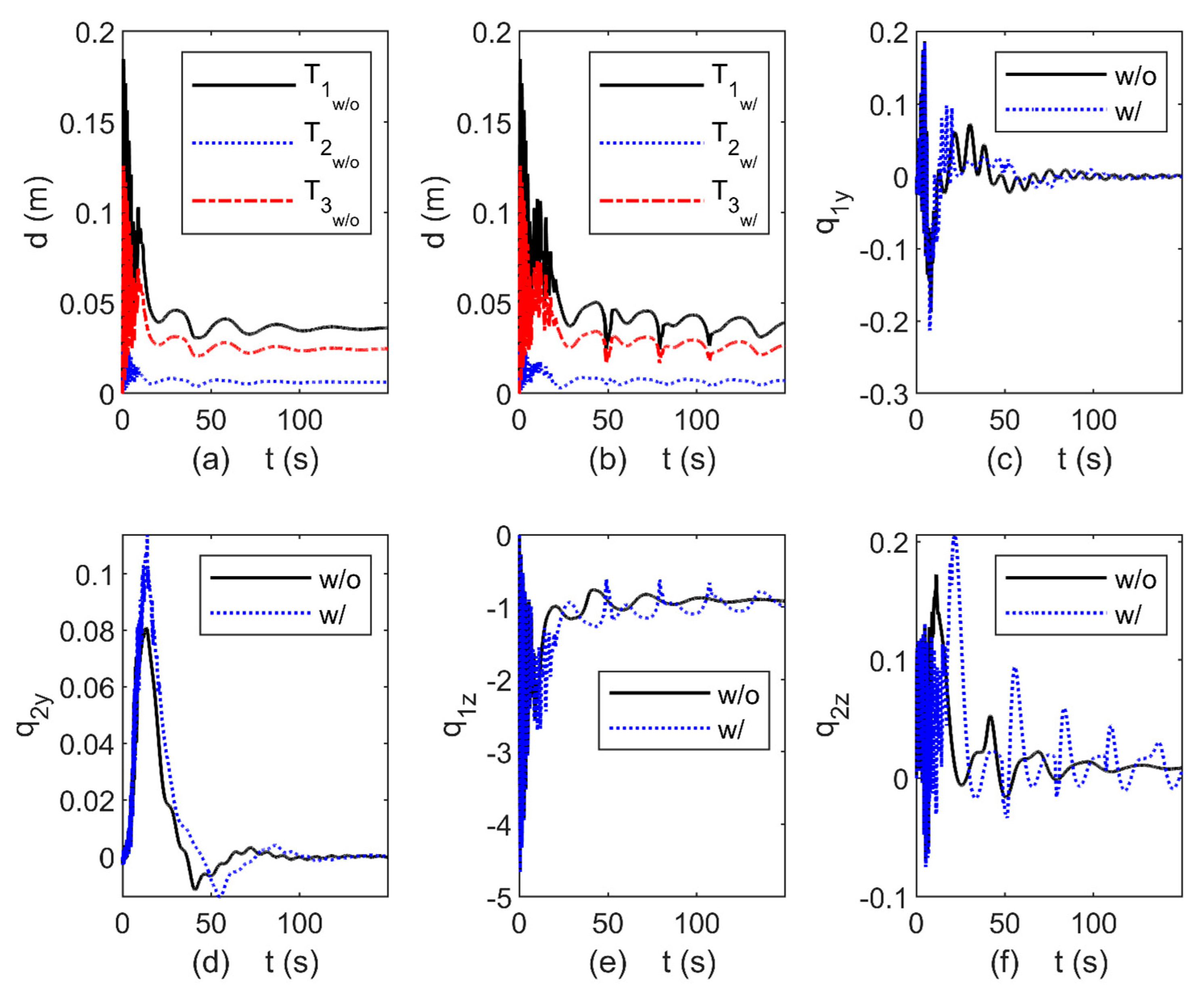
As shown in Figure 12b and Figure 13e, there is strong coupling between pitch and elasticity. Achieving elasticity suppression would result in a coupled pitch angle. To control the pitch angle, a significant amount of force would be required. However, since the thrust capacity is already saturated, it becomes impossible to simultaneously suppress both pitch and elasticity. Figure 18 and Figure 19 present comparison results of elastic control with (w/) and without (w/o) pitch control. The controller parameters for trajectory tracking with elastic suppression are as follows:

$$K_{\mathrm{P}}=\mathrm{diag}\left(\left[\begin{array}{cccccccccc}0.2& 0.1& 6& 10& 4& 2& 0& 0& 70& 0\end{array}\right]\right)$$

$$K_{\mathrm{D}}=\mathrm{diag}\left(\left[\begin{array}{cccccccccc}4& 2& 1& 4& 5& 20& 0& 0& 5& 0\end{array}\right]\right)$$

It can be observed that satisfactory trajectory tracking is achieved in both cases. However, because the thrust has already saturated, the servo-elastic control induces a pitch angle, yet the vehicle possesses no additional pitch control authority—rendering pitch control nearly ineffective. Moreover, pitch control excites significant oscillations in the elastic variable, pitch angle, and altitude error (approximately 1 m), as evidenced in Figure 18f and Figure 19b,d.

4.3. Limitations and Future Work

The servo-elastic control strategy presented in this section demonstrates effective trajectory tracking and significant suppression of elastic deformation in the y_b-direction. However, several limitations arise primarily due to actuator saturation. As shown in Figure 14 and Figure 15, both trajectory tracking controller and SEC controllers operate near or at maximum thrust capacity during maneuvering. This saturation fundamentally restricts the system’s ability to simultaneously achieve pitch control and elastic deformation suppression—as illustrated in Figure 18 and Figure 19—and is evidenced by the persistent pitch offset (approximately 0.59 rad) observed in both control configurations.

Moreover, the airship’s inherent under actuation—specifically the lack of direct lateral force generation—renders channels 2, 7, and 8 uncontrollable (Figure 16), limiting full-state elastic compensation. The reliance on a linear disturbance observer also introduces transient estimation errors during rapid maneuvers (Figure 17), though steady-state accuracy remains acceptable.

To address these challenges, future work will focus on the following directions:

Control Allocation Optimization: Revising the thrust allocation strategy to better exploit available actuation redundancy (e.g., through adaptive or energy-aware allocation) and decouple critical motion channels.

Enhanced Disturbance Estimation: Integrating higher-order or nonlinear disturbance observers to improve transient estimation accuracy during aggressive maneuvers.

Structural Stiffness Tuning: Exploring passive design modifications (e.g., stiffer gondola mounting or tailored flexible modes) to reduce the magnitude of servo-elastic coupling from the outset.

5. Conclusions

This paper presents a servo-elastic control framework for multi-propeller airships that simultaneously achieves accurate trajectory tracking and active suppression of structural deformation. By integrating flight dynamics with a fluid–structure interaction dynamic model derived via Lagrange’s equations, the approach explicitly captures the coupling between hull flexibility and vectoring actuator dynamics. A disturbance observer estimates deformation-induced force deviations at propeller mounting points, enabling real-time compensation and effective vibration mitigation.

Simulation results demonstrate that the proposed method reduces elastic deflection by up to 90% compared to a baseline trajectory tracking controller without deformation compensation, while improving trajectory tracking accuracy by 19% (measured by RMS position error over a 300 s maneuver). Importantly, the study reveals that actuator configuration and vectoring capability critically influence control authority over dominant structural modes, highlighting the need for co-design of propulsion layout and control architecture.

While the current framework demonstrates effective vibration suppression, its theoretical maturity can be enhanced by addressing inherent modeling decoupling and control limitations. Currently, the approach relies on offline Workbench-based FSI simulations for aerodynamic look-up tables and online reduced-order modal superposition for deformation estimation. Although this approach is fast, it sacrifices accuracy during rapid maneuvers because the pre-computed aerodynamic tables cannot capture how real-time structural deformations instantly change the airflow. Furthermore, the manual tuning of the 10-channel PID gains is time-consuming and lacks scalability. To address these issues, future work will focus on: (1) developing an online coupled FSI-flight dynamics solver that embeds structural deformation equations directly into the fluid mechanics loop, thereby eliminating pre-computed coefficients and redundant modal assumptions; (2) transitioning to a unified control allocation strategy (e.g., LQR or MPC) to automatically coordinate multi-vectoring propellers with aerodynamic surfaces across flight speeds; and (3) validating these advanced models and automated control strategies through rigorous experimental verification.

References

1. Lee, M.; Smith, S.; Androulakakis, S. The High Altitude Lighter Than Air Airship Efforts at the US Army Space and Missile Defense Command/Army Forces Strategic Command. In Proceedings of the 18th AIAA Lighter-Than-Air Systems Technology Conference; AIAA 2009-2852; AIAA: Reston, VA, USA, 2012. [Google Scholar]
2. Kohno, T.; Nakadate, M.; Okuvama, M. On-Going UAV R&D at JAXA’s Aviation Program Group-Second Report With Emphasis on LTA Flight Control. In Proceedings of the 18th AIAA Lighter-Than-Air Systems Technology Conference; AIAA 2009-2860; AIAA: Reston, VA, USA, 2012. [Google Scholar]
3. Nickol, C.; Guynn, M.; Kohout, L.; Ozoroski, T. High Altitude Long Endurance Air Vehicle Analysis of Alternatives and Technology Requirements Development. In Proceedings of the 45th AIAA Aerospace Sciences Meeting and Exhibit; AIAA 2007-1050; AIAA: Reston, VA, USA, 2012. [Google Scholar]
4. Bessert, N.; Frederich, O. Nonlinear Airship Aeroelasticity. J. Fluids Struct. 2005, 21, 731–742. [Google Scholar] [CrossRef]
5. Bennaceur, S.; Azouz, N.; Boukraa, D. An Efficient Modelling of Flexible Airships. In Proceedings of the 8th Biennial ASME Conference on Engineering Systems Design and Analysis, Fairfield, NJ, USA, 4–7 July 2006; pp. 573–582. [Google Scholar]
6. Liu, J.M.; Lu, C.J.; Xue, L.P. Investigation of Airship Aeroelasticity Using Fluid Structure Interaction. J. Hydrodyn. 2008, 20, 164–171. [Google Scholar] [CrossRef]
7. Zhang, M.H.; Wang, X.L.; Duan, D.P. Panel Method Predictions of Added Mass for Flexible Airship. Aeronaut. J. 2013, 177, 519–531. [Google Scholar] [CrossRef]
8. Li, X.; Fang, X.; Dai, Q. Research on Thermal Characteristics of Photovoltaic Array of Stratospheric Airship. J. Aircr. 2011, 48, 1380–1386. [Google Scholar] [CrossRef]
9. Li, Y.W.; Nahon, M.; Sharf, I. Dynamics Modeling and Simulation of Flexible Airships. AIAA J. 2009, 47, 592–605. [Google Scholar] [CrossRef]
10. Chen, L.; Whidborne, J.F.; Dong, Q.; Duan, D.; Liu, J. Degraded planary tracking control of an omni-directional vectored-thruster aerostat. ASCE’s J. Aerosp. Eng. 2019, 32. [Google Scholar] [CrossRef]
11. Schmidt, D.K. Modeling and Near-Space Station-Keeping Control of a Large High-Altitude Airship. J. Guid. Control. Dyn. 2007, 30, 540–547. [Google Scholar] [CrossRef]
12. Chen, L.; Dong, Q.; Yan, Z.; Liu, J. Actuator fault modeling and fault-tolerant tracking control of multi-vectored propeller aerostat. Aeronaut. J. 2022, 126, 1982–1996. [Google Scholar] [CrossRef]
13. Han, D.; Yan, L.; Yan, G.; Wang, X.; Duan, D. Integral Command Filtered Backstepping Control of a Flexible UAV. MATEC Web Conf. 2018, 160, 05005. [Google Scholar] [CrossRef]
14. Chen, L.; Gao, Q.Y.; Deng, Y.X.; Liu, J. Moving-mass based station keeping of stratospheric airships. Aeronaut. J. 2021, 125, 1231–1244. [Google Scholar] [CrossRef]
15. Azinheira, J.R.; Moutinho, A.; de Paiva, E.C. Airship Hover Stabilization using a Backstepping Control Approach. J. Guid. Control. Dyn. 2006, 29, 903–914. [Google Scholar] [CrossRef]
16. Sun, Z.W.; Haghighat, S.; Liu, H.H.T.; Bai, J. Time-domain Modeling and Control of a Wing-section Stall Flutter. J. Sound Vib. 2015, 340, 221–238. [Google Scholar] [CrossRef]
17. Wang, W.; Zhu, X.; Zhou, Z.; Duan, J. A Method for Nonlinear Aeroelasticity Trim and Stability Analysis of Very Flexible Aircraft based on Co-rotational Theory. J. Fluids Struct. 2016, 62, 209–229. [Google Scholar] [CrossRef]
18. Gao, W.; Liu, Y.; Li, Q.; Lu, B. Gust load alleviation of a flexible flying wing with linear parameter-varying modeling and model predictive control. Aerosp. Sci. Technol. 2024, 155, 109671. [Google Scholar] [CrossRef]
19. Mozaffari-Jovin, S.; Firouz-Abadi, R.D.; Roshanian, J. L1 adaptive aeroelastic control of an unsteady flapped airfoil in the presence of unmatched nonlinear uncertainties. J. Sound Vib. 2024, 578, 118334. [Google Scholar] [CrossRef]
20. Vindigni, C.R.; Mantegna, G.; Orlando, C.; Alaimo, A. Simple adaptive wing-aileron flutter suppression system. J. Sound Vib. 2024, 570, 118151. [Google Scholar] [CrossRef]
21. Chen, L.; Dong, Q.; Zhang, G.C.; Duan, D. Composite Control System of Hybrid-driven Mid-altitude Airship. Aeronaut. J. 2018, 122, 173–204. [Google Scholar] [CrossRef]
22. Chen, L.; Song, Z.; Lin, J. Dynamics and control of a high-altitude balloon with slung load. Aeronaut. J. 2024, 128, 2856–2878. [Google Scholar] [CrossRef]
23. Lin, J.; Song, Z.; Chen, L. Research on Modal Analysis and Prediction of Flexible Airship. In Proceedings of the 44th Chinese Control Conference, Chongqing, China, 28–30 July 2025. [Google Scholar]
24. Chen, L.; Chen, W.; Li, S.; Zhao, B. Modal characteristics of a scaling stratospheric airship in still air. Aerosp. Sci. Technol. 2023, 141, 108521. [Google Scholar] [CrossRef]
25. Liu, J.M.; Lu, C.J.; Xue, L.P. Numerical investigation on the aeroelastic behavior of an airship with hull-fin configuration. J. Hydrodyn. 2010, 22, 207–213. [Google Scholar] [CrossRef]
26. Chen, W.H.; Yang, J.; Guo, L.; Li, S. Disturbance observer based control and related methods: An overview. IEEE Trans. Ind. Electron. 2015, 63, 1083–1095. [Google Scholar]
Figure 1. Overall structure and propeller configuration of the airship (The labels T1–T6 denote the installation positions of the vectored propellers. The dashed circle highlights a representative vectored position of the propeller. Other symbols are defined in the main text).
Aerospace 13 00275 g001
Figure 2. First eight modal shapes of the airship along with their natural frequencies (Color gradients denote relative displacement magnitudes (red for maximum, blue for minimum): Breathing mode involves local envelope expansion and contraction; Multi-phase breathing features these radial deformations with varying phases along the longitudinal axis; Multi-sided breathing exhibits synchronous axial deformation with multiple circumferential lobes; Torsional mode represents twisting about the longitudinal axis; Axial mode corresponds to longitudinal stretching and compression; and bending mode depicts a beam-like curvature with two half-waves along the structure).
Aerospace 13 00275 g002
Figure 3. Fluid–structure interaction (FSI) analysis framework for the airship.
Aerospace 13 00275 g003
Figure 4. Hull deformation at selected points during the iterative fluid–structure interaction (FSI) process under different air conditions.
Aerospace 13 00275 g004
Figure 5. Convergence history of aerodynamic force and moment coefficients during the iterative fluid–structure interaction (FSI) process under V = 10 m/s, α = 0° and β = 30° (The red dashed line represents the steady-state value).
Aerospace 13 00275 g005
Figure 6. Propeller position variation under the assumed envelope deformation (top view, A, B, C, D, E denotes the propeller mounting position before deformation, and A′, B′, C′, D′, E′ denotes the propeller mounting position after deformation. τ represents the deflection moment, and ε represents the deflection angle of the vector axis for propeller installation.).
Aerospace 13 00275 g006
Figure 7. Propeller reference frame and its modification due to structural deformation.
Aerospace 13 00275 g007
Figure 8. Solution process of fluid–structure interaction dynamics.
Aerospace 13 00275 g008
Figure 9. General structure of the control system.
Aerospace 13 00275 g009
Figure 10. Elastic states of fluid–structure interaction dynamics under different airspeeds.
Aerospace 13 00275 g010
Figure 11. Flight states of fluid–structure interaction dynamics under different airspeeds.
Aerospace 13 00275 g011
Figure 12. Attitude and trajectory tracking.
Aerospace 13 00275 g012
Figure 13. Displacement of the propeller installation positions and the suppression results of the generalized variables.
Aerospace 13 00275 g013
Figure 14. Variation in the deflection angle of a single propeller.
Aerospace 13 00275 g014
Figure 15. Variation in the thrust magnitude of a single propeller.
Aerospace 13 00275 g015
Figure 16. Comparison of control forces and actual output forces with elastic compensation.
Aerospace 13 00275 g016
Figure 17. Time history of the estimated disturbance.
Aerospace 13 00275 g017
Figure 18. Elastic state of elastic control with or without pitch control.
Aerospace 13 00275 g018
Figure 19. Flight states of elastic control with or without pitch control.
Aerospace 13 00275 g019