A Spatio-Temporal Foresight Reinforcement-Learning Framework for Long-Term Station-Keeping of Stratospheric Airships

Abstract

Long-term station-keeping of stratospheric airships is challenged by strong time-varying wind fields, pronounced vertical stratification of wind speed and direction, and limited onboard energy. Existing reinforcement-learning approaches typically rely on instantaneous observations to make reactive decisions and therefore struggle to deliver foresighted control in dynamic environments. This paper proposes a Spatio-Temporal Foresight Reinforcement-Learning framework (STF-RL) that explicitly incorporates future wind information. A Transformer is introduced to model multi-step, multi-altitude forecast wind sequences, and a time–height dual positional encoding is designed to characterize both the temporal evolution and the vertical structure of the wind field. A task-conditioned attention pooling mechanism then extracts the future-wind features most relevant to the current state, which are concatenated with the airship state and fed into an actor–critic network to enable foresighted policy learning. A continuous action space supporting three-dimensional maneuvering is constructed, together with a multi-objective reward that jointly accounts for station-keeping performance, energy consumption and safety. Experimental results show that the proposed method outperforms baseline approaches in station-keeping performance, trajectory stability and energy-utilization efficiency, while exhibiting strong robustness across different wind-field conditions.

1. Introduction

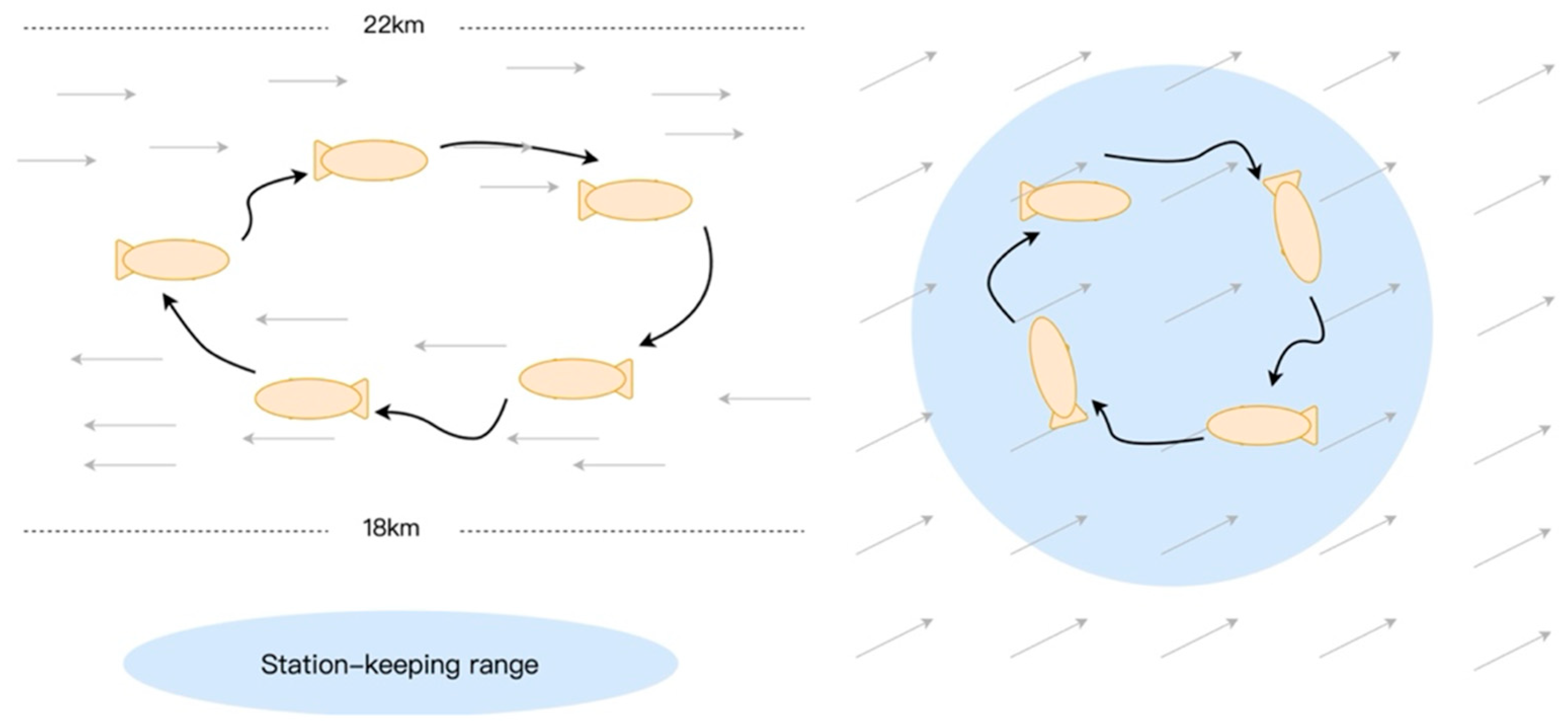
Stratospheric airships generally operate at altitudes of approximately 18–22 km and offer long endurance, deployment flexibility and substantial payload capacity. Their potential value for communication relay and broadband coverage missions has been systematically discussed in early studies [1,2], and the development status and technological trends of these platforms have been reviewed comprehensively [3]. In practical missions, an airship is required to maintain long-term, stable station-keeping above a target region while sustaining effective coverage in a complex and highly variable upper-atmosphere environment. Owing to the coupled influence of wind disturbances, environmental uncertainty and mission constraints [4,5], achieving stable and efficient station-keeping in such environments has become one of the core problems limiting the operational performance of high-altitude platforms. Autonomous station-keeping path planning under complex environmental conditions has therefore emerged as a key research issue for stratospheric airships and related high-altitude platforms.

Unlike conventional path-planning tasks, stratospheric airship station-keeping is simultaneously affected by dynamic wind fields and energy constraints. On the one hand, stratospheric winds exhibit pronounced time variability, non-stationarity and vertical stratification, with significant differences in wind speed and direction across altitude layers and continuous evolution over time [6,7,8,9]. Because an airship has a large windward area and limited maneuverability, its motion is highly sensitive to wind disturbances, which can lead to trajectory drift, increased control cost and degraded station-keeping performance. On the other hand, an airship typically relies on combined solar and battery power, with the propulsion, control and payload subsystems all subject to a limited energy budget; the day–night cycle further intensifies the coupling between energy harvesting and energy consumption [10,11,12,13]. Long-term path planning that simultaneously addresses station-keeping accuracy, disturbance rejection and energy feasibility under time-varying wind conditions therefore remains a challenging research problem.

For path-planning problems, classical methods are mainly grouped into graph-search, sampling-based and evolutionary-optimization approaches. Graph-search methods such as A* and Dijkstra [14,15] offer good determinism and interpretability in static or low-dimensional settings, but they suffer from high computational cost and poor real-time performance in large-scale dynamic environments. Sampling-based methods such as RRT, RRT* and PRM [16,17,18] are capable of higher-dimensional feasible-path search, and an improved RRT method tailored to the constraint set of stratospheric airships [19] further illustrates the engineering potential of this family of approaches; however, their performance is sensitive to environmental complexity and replanning frequency, and their stability is limited under strongly time-varying conditions. Evolutionary-optimization methods such as genetic algorithms, particle-swarm optimization and simulated annealing can address non-convex problems, but they are commonly hampered by parameter sensitivity, slow convergence and limited dynamic adaptability. Overall, traditional path-planning methods have difficulty in jointly handling the persistent evolution of stratospheric winds, the continuous control requirements of the airship, and the coupling imposed by long-term energy constraints.

Deep reinforcement learning has recently provided a new technical pathway for autonomous path planning in complex dynamic environments. Value-based methods exemplified by DQN [20], double Q-learning [21] and DRQN [22] have extended the applicability of reinforcement learning to partially observable and high-dimensional decision-making tasks, while PPO [23] and SAC [24] have further improved training stability and sample efficiency in continuous-control tasks. These approaches have recently been adopted for stratospheric airship path planning under dynamic winds [25,26,27,28]. In particular, long-horizon hierarchical reinforcement-learning planning [29], fixed-time trajectory planning [30] and deep reinforcement-learning methods designed for spatio-temporally complex environments [31] have improved policy foresight and robustness in complex wind fields. Related ideas have been extended to resource-constrained high-altitude balloon station-keeping [32,33,34] and multi-airship formation coverage missions [35,36,37], showing that reinforcement learning can yield flight policies with reasonable robustness under wind disturbances and continuous control. Compared with the classical approaches above, reinforcement learning is better suited to closed-loop decision-making problems characterized by uncertainty and long temporal horizons.

Despite this progress, existing reinforcement-learning-based airship path-planning studies still exhibit clear limitations. First, prior work has shown that external numerical weather prediction systems and large-scale wind-field datasets can already provide usable future-wind priors for stratospheric airship missions [6,7,38]. Nevertheless, many path-planning methods for dynamic wind fields still update their policies primarily on the basis of current local observations [25,26,27,28,29,30,31] and thus follow a typical reactive control paradigm. Even in studies that incorporate wind information, future-wind priors are often treated only as background context or local auxiliary information, rather than being organized into a unified, task-relevant representation. For wind environments with pronounced temporal evolution, such methods can respond to short-term disturbances but cannot explicitly exploit future environmental trends, leading to myopic decisions that struggle to balance trajectory stability and energy efficiency over long station-keeping missions. Second, prior work on forecast-wind-based path planning, recovery trajectory optimization, horizontal trajectory control and regional station-keeping [6,7,39,40], together with studies on station-keeping control and policy optimization in dynamic winds [11,13], has shown that the key control dimensions of stratospheric station-keeping involve not only horizontal maneuvering but also altitude adjustment. Because wind structures often differ markedly across altitude layers, a well-designed altitude-changing strategy can effectively avoid unfavorable flows and exploit advantageous wind layers, thereby improving station-keeping feasibility and reducing energy consumption. Although recent work has begun to introduce temporal perception and dual-source learning mechanisms [41], a unified, task-relevant representation of future multi-altitude wind fields remains to be further developed.

From a task-mechanism perspective, station-keeping decision-making for a stratospheric airship must answer at least the following two interrelated questions: how the wind field at each altitude will evolve over the coming horizon, and how the airship should exploit this spatio-temporal heterogeneity to perform foresighted horizontal motion and altitude adjustment under the current energy state and mission constraints. If the policy model lacks an effective representation of the joint temporal–vertical structure of future winds, it can hardly form genuinely global decisions for long-term station-keeping. It is therefore necessary to introduce representation-learning methods capable of capturing long-range temporal dependencies and inter-layer correlations, so as to extract from external forecast winds the environmental features most relevant to the current control decision and to integrate them deeply into the reinforcement-learning policy-optimization process.

As a classical sequence model, LSTM [42] laid an important foundation for subsequent sequence-modeling research, while the Transformer, built on the self-attention mechanism [43], can effectively model long-range dependencies in long sequences. Studies on multivariate time-series representation learning [44], together with long-sequence forecasting models such as Informer, Autoformer and the Temporal Fusion Transformer [45,46,47], have further demonstrated that attention-based architectures can effectively capture complex cross-step dependencies. For stratospheric airship path planning, future winds inherently possess a dual temporal–altitudinal structure as follows: the wind state evolves continuously in time, and clear differences and potential synergies exist among altitude layers. The Transformer therefore provides a suitable technical foundation for the unified representation of future multi-altitude wind fields.

Building on the considerations above, this paper proposes a Transformer-aware reinforcement-learning path-planning method for long-term station-keeping of stratospheric airships. Rather than performing generative wind prediction, the method directly exploits future-wind information provided by external numerical weather prediction systems and reanalysis data [38] and uses a Transformer to learn task-relevant spatio-temporal features. To strengthen the model’s ability to discriminate wind structures, a time–height dual positional encoding is designed to explicitly model future temporal information and vertical-layer information. On this basis, a Transformer encoder learns a joint representation of multi-step, multi-altitude future winds, and a task-conditioned pooling mechanism produces a compact environmental feature aligned with the current airship state. This wind latent representation is then combined with the airship’s current position, flight state and remaining energy and fed into the reinforcement-learning policy network, enabling tightly coupled perception and decision-making. The framework supports foresighted altitude-changing station-keeping under complex wind and energy constraints while accounting for long-term energy sustainability [48].

The main contributions of this work are summarized as follows.

First, a spatio-temporal representation mechanism for future multi-altitude winds is proposed. To address the joint temporal evolution and vertical stratification of stratospheric winds, a structured input representation indexed by both time and altitude is constructed, and a time–height dual positional encoding is designed to enhance the model’s ability to discriminate the spatio-temporal structure of the wind field.

Second, a decision-making framework that couples Transformer-based perception with reinforcement-learning policy optimization is developed. By sharing the wind encoder and the task-conditioned pooling mechanism, both the policy network and the value network can extract future-wind features most relevant to the current task state, alleviating the myopia caused by classical reinforcement-learning approaches that rely solely on instantaneous observations.

Third, for the three-dimensional station-keeping control task, a continuous action space supporting both horizontal maneuvering and altitude adjustment is designed. The reward function jointly considers target station-keeping, the energy state and safety constraints, enabling the policy to actively select more advantageous flight altitudes in complex wind fields and to achieve a coordinated optimization of station-keeping performance and energy feasibility.

Beyond the technical formulation, stratospheric-platform deployment is also shaped by emerging regulatory and operational standardization efforts. Internationally, ITU discussions on HAPS/HIBS spectrum identification and coordination, together with ICAO work on the integration of unmanned and advanced aviation operations, indicate that future high-altitude operations will need clearer rules for communications, airspace safety and operational approval [49,50]. In China, relevant frameworks are likely to involve coordinated development among civil-space, aviation, spectrum-management and aerospace-standardization authorities, including bodies such as CNSA, SAMR and CAAC [51,52,53]. Improved station-keeping reliability and predictable energy-aware operation can therefore provide a technical basis for future standardized and certifiable stratospheric-platform missions.

The remainder of the paper is organized as follows. Section 2 presents the environment model and the formulation as a Markov decision process. Section 3 describes the proposed planning framework in detail, including the Transformer-based wind modeling, the perception-decision mechanism, and the altitude-changing dynamic strategy. Section 4 reports the experimental setup and result analysis. Section 5 discusses limitations and future work, and Section 6 concludes the paper.

2. Problem Formulation

2.1. Environment Modeling

This work addresses the long-term regional station-keeping problem of a stratospheric airship in a complex, time-varying wind field. The objective is to autonomously regulate the airship’s horizontal propulsion, heading and altitude under given target-region and energy constraints, so that the airship remains in the vicinity of the target region for as long as possible, as illustrated in Figure 1, while jointly maintaining energy sustainability and flight safety. Unlike conventional two-dimensional path planning, this task is simultaneously affected by the spatio-temporal evolution of the wind field, inter-layer wind differences and the diurnal energy cycle, and is therefore inherently a three-dimensional sequential decision-making problem driven by the coupling between a dynamic environment and resource constraints.

Because this study focuses on mission-level path planning rather than on the high-frequency attitude response of low-level flight control, the environment is modeled with a simplified three-dimensional kinematic description. The formulation retains only the state-evolution factors directly relevant to decision-making, namely changes in airship position, the influence of wind disturbances and the dynamics of the energy state. It thereby reduces environmental complexity while preserving physical plausibility, providing a stable, controllable and representative interactive platform for reinforcement-learning policy training.

This simplification is adopted for the physical scale considered in this work. The decision interval is 300 s, and each episode covers 72 h, so the reinforcement-learning agent operates at the mission-planning level rather than at the inner-loop attitude-control level. Over this time scale, the dominant state-evolution mechanisms are the advection induced by stratospheric wind, the commanded horizontal airspeed and heading, the slowly varying altitude command, and the charging-discharging energy balance. High-frequency aerodynamic effects, actuator transients, structural elasticity and attitude dynamics are therefore treated as lower-level control effects that are assumed to be stabilized by the onboard flight-control system.

The model should consequently be interpreted as a mission-level kinematic planning model, not as a replacement for a six-degree-of-freedom aerodynamic simulator. This abstraction is consistent with the objective of comparing foresighted station-keeping policies under identical wind, energy and action constraints. To make the abstraction explicit, Figure 2 defines the reference frame, vectors and angles used throughout the formulation. The aerodynamic influence of vehicle size is retained indirectly through the physically bounded speed, vertical-rate, action-smoothness and propulsion-power constraints, while higher-fidelity aerodynamic force and moment modeling is left for hardware-in-the-loop or flight-test validation.

2.1.1. Airship Kinematic Model

Let the spatial position of the airship at time $t$ be denoted as

$${\mathbf{p}}_t={\left[x_t,y_t,z_t\right]}^{\mathrm{\top }}$$

(1)

where $x_t$ and $y_t$ are the horizontal coordinates and $z_t$ denotes the flight altitude. The control inputs of the airship comprise the horizontal propulsion speed $v_t$ relative to the airflow, the heading angle ${\psi }_t$, and the vertical speed $v_{z,t}$. Neglecting high-frequency details such as attitude variation, structural elasticity and actuator hysteresis, the three-dimensional motion of the airship can be expressed as

$${\dot{\mathbf{p}}}_t=\left[\begin{array}{c}{v}_t\mathrm{c}\mathrm{o}\mathrm{s}{\psi }_t\\ v_t\mathrm{s}\mathrm{i}\mathrm{n}{\psi }_t\\ v_{z,t}\end{array}\right]+\mathbf{w}\left({\mathbf{p}}_t,t\right)$$

(2)

where $\mathbf{w}\left({\mathbf{p}}_t,t\right)={\left[u\left({\mathbf{p}}_t,t\right),v\left({\mathbf{p}}_t,t\right),w\left({\mathbf{p}}_t,t\right)\right]}^{\mathrm{\top }}$ is the three-dimensional wind-velocity vector at time $t$ and position ${\mathbf{p}}_t$. This term captures the direct influence of the ambient wind on the airship’s ground velocity and represents the principal external disturbance driving the airship away from the target region.

In the model above, the actual motion of the airship is jointly determined by the autonomous control inputs and the ambient wind. Stratospheric winds vary markedly in both time and altitude, and substantial differences in wind speed are commonly observed across altitude layers. The airship therefore not only needs to counteract unfavorable winds through horizontal control but can also actively seek more favorable wind layers via altitude-changing maneuvers, thereby improving station-keeping capability and reducing propulsion cost.

2.1.2. Wind-Disturbance Modeling

Although the ambient wind field can be supplied by external numerical weather prediction and reanalysis data, real upper-atmosphere winds inevitably contain forecasting errors, local disturbances and unmodeled small-scale variations. If only an idealized forecast wind is used during training, the policy is prone to overfit a deterministic environment, weakening its robustness in real deployment. To address this, a stochastic disturbance term is superimposed on the baseline wind field to emulate environmental uncertainty.

Let the baseline wind field be $\mathbf{w}\left({\mathbf{p}}_t,t\right)$. The actual perturbed wind field is then expressed as

$$\tilde{\mathbf{w}}\left({\mathbf{p}}_t,t\right)=\mathbf{w}\left({\mathbf{p}}_t,t\right)+{\mathit{ϵ}}_t$$

(3)

where ${\mathit{ϵ}}_t$ is a zero-mean Gaussian random disturbance, namely

$${\mathit{ϵ}}_t\sim \mathcal{N}\left(\mathbf{0},\Sigma \right)$$

(4)

with the covariance matrix taken in diagonal form

$$\Sigma =\mathrm{d}\mathrm{i}\mathrm{a}\mathrm{g}\left({\sigma }_x^2,{\sigma }_y^2,{\sigma }_z^2\right)$$

(5)

where ${\sigma }_x, {\sigma }_y$ and ${\sigma }_z$ denote the disturbance intensities along the three directions, respectively. This setting approximates non-deterministic factors such as wind-speed measurement errors, short-term forecast biases and small-scale local disturbances. The kinematic equation of the airship can therefore be further written as follows.

In the present experiments, the covariance is kept diagonal and constant with altitude to isolate the effect of the proposed decision-making architecture from additional uncertainty-modeling factors. Physically, this term represents a compact approximation of forecast error, measurement error and unresolved local fluctuations around the ERA5-based background wind. We acknowledge that real stratospheric forecast uncertainty and turbulence intensity are altitude dependent and may also exhibit cross-component correlations. A more detailed deployment model can replace the constant covariance with an altitude-dependent covariance Sigma (z) estimated from forecast-error statistics, but this extension is beyond the scope of the current algorithm-comparison study.

$${\dot{\mathbf{p}}}_t=\left[\begin{array}{c}{v}_t\mathrm{c}\mathrm{o}\mathrm{s}{\psi }_t\\ v_t\mathrm{s}\mathrm{i}\mathrm{n}{\psi }_t\\ v_{z,t}\end{array}\right]+\tilde{\mathbf{w}}\left({\mathbf{p}}_t,t\right)$$

(6)

2.1.3. Energy-Constraint Model

For long-term station-keeping missions, the path planning of a high-altitude airship cannot be optimized solely with respect to geometric proximity to the target or maintenance of the target region; the dynamic evolution of the energy state and the diurnal energy cycle must also be taken into account. Unlike short-endurance vehicles, an airship typically relies on the joint operation of solar cells and batteries, and its propulsion, control and avionics subsystems continuously consume the limited stored energy. If energy constraints are ignored, a policy may temporarily improve station-keeping performance through high-frequency, high-thrust control, only to rapidly deplete the battery during the night or under sustained headwinds, ultimately failing the mission.

Let the remaining energy of the airship at time $t$ be $E_t$. Its dynamics are jointly determined by the energy input and the energy consumption, namely

$${\dot{E}}_t=P_{\mathrm{in}}\left(t\right)-P_{\mathrm{out}}\left(t\right)$$

(7)

where the energy consumption mainly comprises the power drawn by the propulsion system and the avionics. Considering that the propulsion power required to sustain flight is generally a non-linear function of speed, the propulsion power is approximated as

$$P_{\mathrm{prop}}\left(t\right)=k_p{‖{\mathbf{v}}_t‖}^3$$

(8)

where $k_p$ is a coefficient related to the airship’s aerodynamic characteristics and propulsion efficiency; ${\mathbf{v}}_t$ is the airspeed vector. The continuous power consumption of the avionics is denoted by the constant $P_{\mathrm{a}\mathrm{v}}$. The total output power is therefore

$$P_{\mathrm{o}\mathrm{u}\mathrm{t}}\left(t\right)=P_{\mathrm{p}\mathrm{r}\mathrm{o}\mathrm{p}}\left(t\right)+P_{\mathrm{a}\mathrm{v}}$$

(9)

The energy input is provided primarily by the onboard solar panels. Let the solar irradiance be $I_t$, the photovoltaic conversion efficiency be $\eta$, and the effective receiving area be $A$. The instantaneous charging power is then

$$P_{\mathrm{i}\mathrm{n}}\left(t\right)=\eta A{I}_t\xi \left(t\right)$$

(10)

where $\xi \left(t\right)\in [0,1]$ is a solar-availability factor that captures the periodic variation in solar irradiance under the diurnal cycle. To reflect the daily cycle, $\xi \left(t\right)$ is approximated by a periodic function that takes high values during the day and decays to zero at night, thereby emulating the diurnal fluctuation of solar-energy supply.

With a discrete time step $\Delta t$, the energy state is updated as

$$E_{t+1}=E_t+\Delta t\left(P_{\mathrm{i}\mathrm{n}}\left(t\right)-P_{\mathrm{o}\mathrm{u}\mathrm{t}}\left(t\right)\right)$$

(11)

To guarantee mission sustainability and system safety, lower and upper bounds are imposed on the energy state. When the remaining energy approaches the safety lower bound, the policy must give priority to reducing energy consumption and exploiting favorable wind layers to recover the energy reserve, rather than merely sustaining the local position by means of high-thrust control. The station-keeping problem is thus further characterized as a coupled optimization problem influenced jointly by the spatio-temporal evolution of the wind field and the resource constraints.

2.2. Markov Decision Process

To formalize the long-term station-keeping control of the airship in a complex wind field, the path-planning task is modeled as a Markov decision process (MDP), denoted as

$$\mathcal{M}=\left(\mathcal{S},\mathcal{A},\mathcal{P},r,\gamma \right)$$

(12)

where $\mathcal{S}$ is the state space, $\mathcal{A}$ is the action space, $\mathcal{P}$ is the state-transition probability, $r$ is the immediate reward function, and $\gamma$ is the discount factor.

At time $t$, the state $s_t\in \mathcal{S}$ is composed of both the current airship state and future-wind information, namely

$$s_t=\left\{s_t^a,{\mathcal{W}}_t\right\}$$

(13)

where $s_t^a$ collects the airship’s current position, flight altitude, speed, heading angle, remaining energy and other state information, and ${\mathcal{W}}_t$ denotes the forecast wind field over a finite future horizon at multiple altitude layers. This state definition allows the agent not only to use current observations, but also to incorporate the predicted evolution of the wind field for foresighted planning.

The action $a_t\in \mathcal{A}$ adopts a continuous-control form and is defined as

$$a_t={\left[v_t,{\psi }_t,v_{z,t}\right]}^{\mathrm{\top }}$$

(14)

where $v_t$ is the horizontal propulsion speed, ${\psi }_t$ is the heading angle, and $v_{z,t}$ is the vertical speed. This action space simultaneously supports horizontal maneuvering and altitude variation, enabling the airship to actively seek more favorable wind layers through altitude switching.

State transitions are jointly determined by the airship kinematics, the wind disturbances and the energy dynamics. Because the wind environment is stochastic and time-varying, no explicit transition function is constructed; instead, transitions are obtained through the agent’s interactions with the simulation environment.

The reward function $r_t=r\left(s_t,a_t\right)$ measures the immediate contribution of the current action to the mission objective. The reward design jointly considers regional station-keeping, progress towards the target, energy constraints and safety requirements, so as to guide the agent towards control policies that balance station-keeping performance and energy efficiency. Its specific form is given later in the paper.

Under this formulation, the optimization goal is to learn an optimal policy ${\pi }^{\ast }\left(a_t\mid s_t\right)$ that maximizes the expected cumulative discounted reward over the entire mission horizon, namely

$${\pi }^{\ast }=\mathrm{a}\mathrm{r}\mathrm{g} \underset{\pi }{\mathrm{m}\mathrm{a}\mathrm{x}} {\mathbb{E}}_{\pi }\left[{\displaystyle \sum _{t=0}^T} {\gamma }^t{r}_t\right]$$

(15)

Building on this formulation, the subsequent sections develop a reinforcement-learning framework that integrates future-wind encoding with continuous-control policy optimization.

3. Proposed Method

3.1. Overall Framework

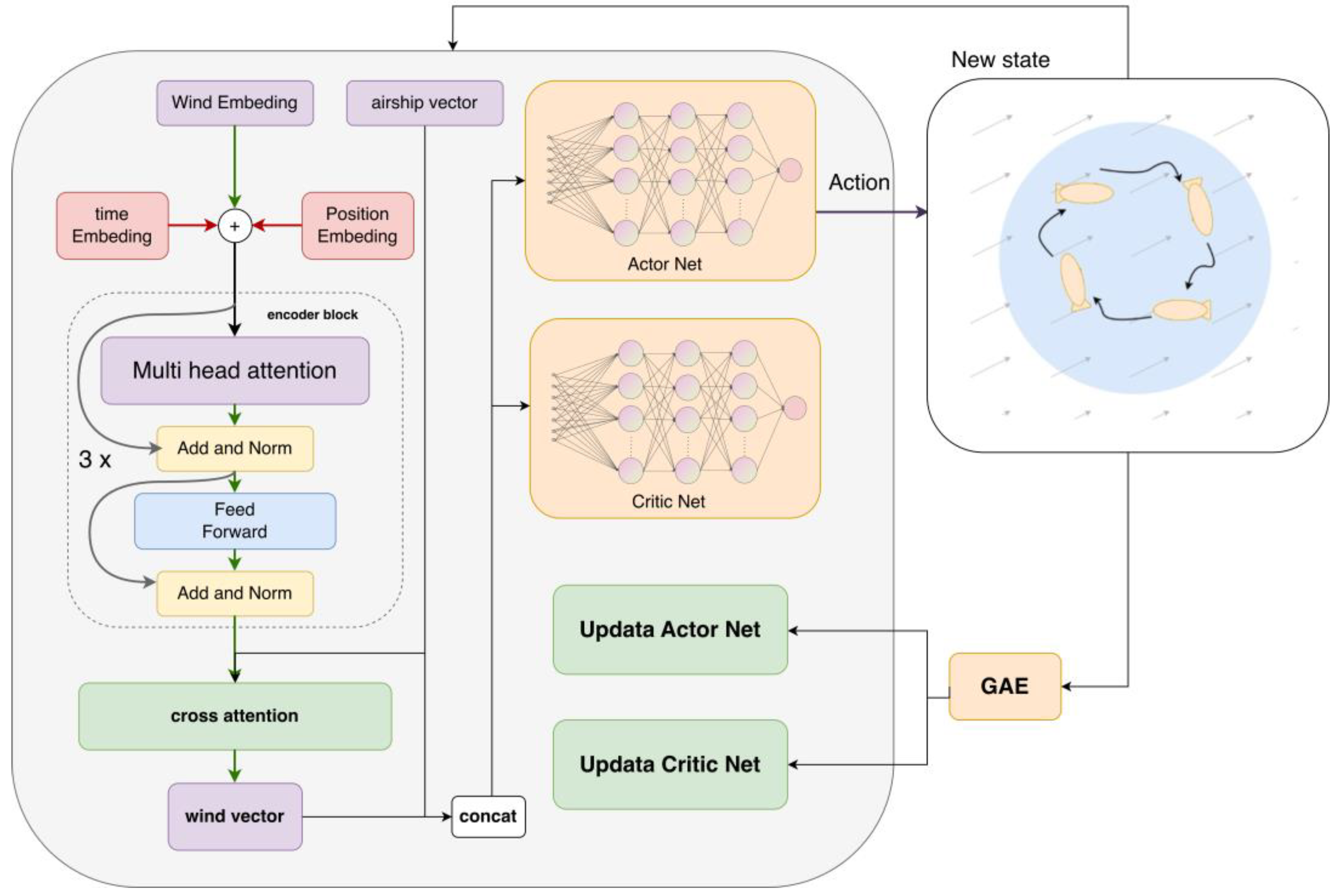
To address the long-term station-keeping path-planning problem of stratospheric airships under complex time-varying winds and energy constraints, this work uses future multi-step, multi-altitude forecast winds as an environmental prior. A Transformer is employed to learn representations of the multivariate time series and, drawing on architectural strengths from long-sequence modeling, to extract the key evolutionary features of the wind field along the temporal and vertical dimensions. Compared with reactive path-planning approaches that rely solely on current observations, the proposed method explicitly exploits future-wind trends during decision-making, thereby providing a more foresighted environmental basis for station-keeping path planning. The overall framework of the proposed method is illustrated in Figure 3.

The method consists of the following four components: future-wind input, spatio-temporal feature encoding, path decision-making and policy optimization. At each decision step, the environment supplies the agent with the airship’s current state together with forecast winds at multiple altitude layers over a finite future horizon. The future-wind tensor is unfolded into a sequence of spatio-temporal tokens, and a time–height dual positional encoding is added to retain the structural information across future time steps and vertical layers. A Transformer encoder then performs unified representation learning on the multi-altitude wind sequence, yielding wind features that incorporate global contextual relationships. A task-conditioned attention pooling mechanism subsequently extracts, from the encoded wind features, the latent representation most relevant to the current station-keeping task. This representation is concatenated with the airship’s current position, leaving energy and target information to form an augmented state input for the reinforcement-learning policy, which is then optimized within the PPO framework.

At the path-planning level, an actor–critic reinforcement-learning structure is used to model the airship’s path decisions. The policy network outputs a continuous action conditioned on the augmented state, representing the path-adjustment decision at the current step, while the value network estimates the long-term return of the current state and provides the basis for policy updates. Because the action space includes both horizontal maneuvering and altitude adjustment, the learned policy can adaptively select more favorable flight layers according to the predicted wind distribution and dynamically refine the path, thereby balancing station-keeping accuracy, path feasibility and energy consumption. The entire framework is trained end-to-end under PPO, allowing wind-field representation learning and path decision-making to be optimized jointly and producing an adaptive station-keeping path-planning policy suited to complex wind environments.

On the basis of this design, a closed-loop methodology that comprises future-wind input, spatio-temporal feature encoding, task-relevant pooling, path-decision output and policy-optimization update is established. Subsequent subsections describe the state representation and future-wind input, the time–height dual positional encoding and the Transformer-based wind encoder, and finally the design of the reinforcement-learning policy network, the action space and the reward function.

3.2. Wind-Field Data Representation

To enable the reinforcement-learning agent to make foresighted decisions in highly variable stratospheric winds, the state space is designed as a joint representation that combines the airship’s current state with future forecast winds. The airship state reflects the current mission conditions, while the future forecast wind provides the predicted evolution of the environment, allowing the agent to leverage both instantaneous observations and environmental priors for adaptive station-keeping path planning.

(1)

Airship state representation.

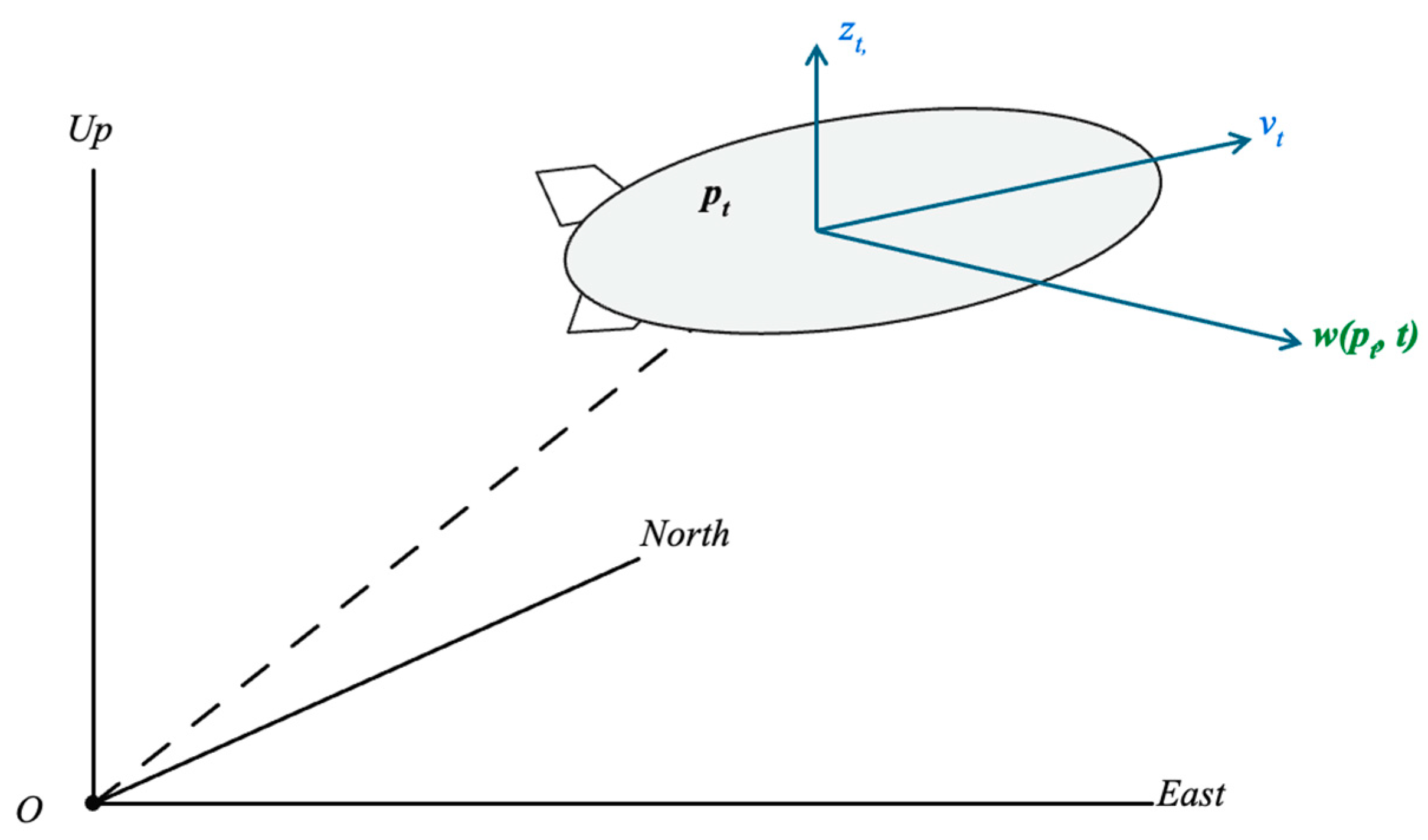
The airship’s current state vector mainly describes its kinematic state, energy state and task-related information at the current time. The airship state at time $t$ is defined as

$$s_{\mathrm{airship}, t}=\left[x_t,y_t,h_t,v_t,{\psi }_t,E_t,x_t^{\mathrm{target}},y_t^{\mathrm{target}}\right]$$

(16)

where $x_t$ and $y_t$ are the horizontal coordinates of the airship, $h_t$ is the current flight altitude, $v_t$ is the airspeed, ${\psi }_t$ is the heading angle, $E_t$ is the remaining energy, and $x_t^{\mathrm{t}\mathrm{a}\mathrm{r}\mathrm{g}\mathrm{e}\mathrm{t}}$ and $y_t^{\mathrm{t}\mathrm{a}\mathrm{r}\mathrm{g}\mathrm{e}\mathrm{t}}$ are the center coordinates of the target station-keeping region. These variables jointly describe the airship’s current dynamic characteristics, mission constraints and available resources, and form the basis for action selection.

Because different state variables differ markedly in physical units and numerical ranges, all state variables are normalized before training to improve the stability and convergence of neural-network training. The normalized airship state vector is denoted by ${\tilde{s}}_{\mathrm{airship},t}$.

(2)

Future-wind representation.

To strengthen the policy’s ability to perceive future environmental changes, the forecast wind over the next 12 h is incorporated into the state space as a key component. It should be emphasized that the wind information used in this work is not predicted by the model itself but is provided by an external numerical weather prediction system. The role of the Transformer module is to encode this forecast wind and extract spatio-temporal features useful for decision-making, rather than to perform wind forecasting.

Let the forecast wind tensor at time $t$, covering $T$ future time steps and $H$ altitude layers, be

$$W_t\in {\mathbb{R}}^{T\times H\times C}$$

(17)

where $T$ is the future forecast horizon, $H$ is the number of vertical layers, and $C$ is the dimensionality of wind features at each spatio-temporal location. In this work, $C=3$, corresponding to the following three wind components: the eastward wind speed $u$, the northward wind speed $v$, and the vertical wind speed $w$. The wind tensor can therefore be expressed as

$$W_t=\left\{w_{t+\tau ,h_j}\mid \tau =1,2,\cdots ,T,j=1,2,\cdots ,H\right\}$$

(18)

where $w_{t+\tau ,h_j}=\left[u_{t+\tau ,h_j},v_{t+\tau ,h_j},w_{t+\tau ,h_j}\right]$ is the wind vector at the $\tau$-th future time step on the $j$-th altitude layer.

To facilitate processing by the subsequent Transformer encoder, the wind tensor is first unfolded along the temporal and altitudinal dimensions into a sequence of spatio-temporal tokens:

$${\widehat{W}}_t\in {\mathbb{R}}^{\left(T\times H\right)\times C}$$

(19)

Each wind token is then projected into a $d$-dimensional feature space via a linear mapping to obtain the wind embedding:

$$X_t={\widehat{W}}_t{W}_e+b_e$$

(20)

where $W_e\in {\mathbb{R}}^{C\times d}$ is a learnable embedding matrix, $b_e$ is a bias term, and $X_t\in {\mathbb{R}}^{(T\times H)\times d}$ is the initial feature representation of the wind tokens.

(3)

Joint state-space representation.

Based on the definitions above, the raw state used at the environment level is

$$s_t=\left\{s_{\mathrm{airship},t},W_t\right\}$$

(21)

i.e., it is composed of both the airship’s current state and the future forecast wind. This state definition departs from classical reinforcement-learning approaches that rely only on current local observations, allowing the agent not only to perceive its current state but also to exploit prior information about how the environment is likely to evolve, thereby improving its adaptability to strongly time-varying wind environments.

However, the raw wind tensor $W_t$ is high-dimensional and exhibits complex spatio-temporal coupling and is therefore unsuitable for direct input to the policy network. To this end, a Transformer-based wind encoder is used to learn its representation, extract the key structural information of the future forecast wind across the temporal and vertical dimensions, and produce a compact wind latent representation $z_{\mathrm{wind},\mathrm{t}}$ through the task-conditioned attention pooling mechanism. On this basis, the augmented state used in the reinforcement-learning decision stage is constructed as

$$s_t^{\ast }=\left[{\tilde{s}}_{\mathrm{airship},t};z_{\mathrm{wind},t}\right]$$

(22)

where $z_{\mathrm{wind},t}$ denotes the task-relevant environmental feature extracted by the wind encoder, reflecting the wind patterns at different future time steps and altitude layers that are most relevant to the current decision; $s_t^{\ast }$ then serves as the input to the actor–critic network for continuous action output and state-value estimation.

3.3. Time–Height Dual Positional Encoding

For stratospheric airship path planning, future winds exhibit pronounced temporal evolution and clearly differ across altitude layers. Without explicitly injecting positional information along the temporal and altitudinal dimensions, a Transformer encoder cannot accurately distinguish between “different altitude layers at the same time” and “the same altitude layer at different future times”, which weakens the model’s ability to represent the spatio-temporal structure of the wind field. To address this, a time–height dual positional encoding (THDPE) is proposed that explicitly models the temporal-order information and the vertical-layer information of the future forecast wind. With this mechanism, during self-attention computation the model not only uses the wind features of each token but also perceives the future time step and altitude layer to which the token corresponds, enabling more accurate learning of the coupled evolution of the wind field along the temporal and vertical dimensions.

Let the future forecast horizon be $T$ and the number of vertical layers be $H$. After unfolding, the $i$-th token uniquely corresponds to a time index ${\tau }_i$ and an altitude index $h_i$. For each wind token, a time positional encoding vector $p_{{\tau }_i}^{\mathrm{time} }\in {\mathbb{R}}^d$ and a height positional encoding vector $p_{h_i}^{\mathrm{height} }\in {\mathbb{R}}^d$ are constructed and added to the wind embedding to form the final input representation to the encoder:

$${\bar{x}}_i=x_i+p_{{\tau }_i}^{\mathrm{time}}+p_{h_i}^{\mathrm{height}},i=1,2,\cdots ,T\times H$$

(23)

Writing all token representations in matrix form yields

$${\bar{X}}_t=X_t+P^{\mathrm{time}}+P^{\mathrm{height}}$$

(24)

where ${\bar{X}}_t\in {\mathbb{R}}^{(T\times H)\times d}$ is the wind feature representation after the dual positional encoding has been added, and $P^{\mathrm{time} }$ and $P^{\mathrm{height} }$ denote the time and height positional encoding matrices broadcast in token order, respectively.

In the implementation, learnable positional encodings are adopted, in which a trainable embedding vector is assigned to each future time step and each altitude layer. The time positional encoding matrix is

$$E^{\mathrm{time}}\in {\mathbb{R}}^{T\times d}$$

(25)

where the $\tau$-th row $E_{\tau }^{\mathrm{time} }$ corresponds to the position representation of the $\tau$-th future time step. The height positional encoding matrix is

$$E^{\mathrm{height}}\in {\mathbb{R}}^{H\times d}$$

(26)

where the $j$-th row $E_j^{\mathrm{height} }$ corresponds to the position representation of the $j$-th altitude layer. For any token, its positional encoding is jointly determined by the corresponding time and height embeddings, namely

$$p_{{\tau }_i}^{\mathrm{time} }=E_{{\tau }_i}^{\mathrm{time}}, p_{h_i}^{\mathrm{height}}=E_{h_i}^{\mathrm{height} }$$

(27)

More explicitly, the implementation uses learnable rather than sinusoidal positional embeddings. Let ${\mathrm{P}}^{time}$ denote a trainable table of size T × d and let ${\mathrm{P}}^{height}$ denote a trainable table of size H × d, where T is the number of future lead times, H is the number of altitude layers and d is the token-embedding dimension. For the token associated with lead time tau and altitude index h, the encoder input is formed by additive fusion as follows: ${\bar{X}}_t=X_t+P^{\mathrm{time} }+P^{\mathrm{height} }$. Thus, the temporal and vertical structural priors have the same feature dimension as the wind embedding and are combined by addition rather than concatenation.

In the reported implementation, T corresponds to the 12 h future-wind window, H = 21 vertical layers and d = 256. The additive design keeps the token dimension unchanged before the Transformer encoder, whereas the separate time and height tables allow the attention module to distinguish whether two tokens differ because of forecast lead time, flight altitude or both. This additional description is included to make the THDPE module fully reproducible.

Compared with a single one-dimensional positional encoding, this dual encoding is better suited to the present setting. With a conventional one-dimensional encoding, the model can only perceive token order in the linearly unfolded sequence and cannot determine whether a given ordering originates from temporal variation or altitudinal variation. By separately encoding the time and altitude indices, the model can more accurately identify the source of wind variation and, in subsequent self-attention computations, learn temporal and inter-layer correlations in a targeted manner.

The time and height positional encodings therefore jointly form a temporal–altitudinal structural prior on the wind tokens, equipping the model input with explicit temporal-order and vertical-layer information before it enters the encoder. On this basis, ideas from sequence modeling are integrated with the Transformer encoder, drawing on design experience from multivariate time-series representation learning and long-sequence modeling, to perform unified modeling of the dependencies of the future forecast wind along the temporal and altitudinal dimensions.

3.4. Transformer-Based Wind Encoder

To accurately extract the coupled evolutionary features of the future forecast wind along the temporal and vertical dimensions, a Transformer-based spatio-temporal wind encoder is constructed. It should be stressed that the Transformer module here does not perform wind forecasting; instead, it learns representations of the 12 h, multi-altitude future-wind sequences provided by an external numerical weather prediction system, from which latent environmental features useful for path planning are extracted. This design allows the agent to exploit future-wind trends explicitly during decision-making, thereby alleviating the myopia caused by reliance on instantaneous observations in classical reinforcement learning.

Let the input sequence after linear embedding and time–height dual positional encoding be

$$X^0=\left[x_1,x_2,\cdots ,x_N\right]\in {\mathbb{R}}^{N\times d}$$

(28)

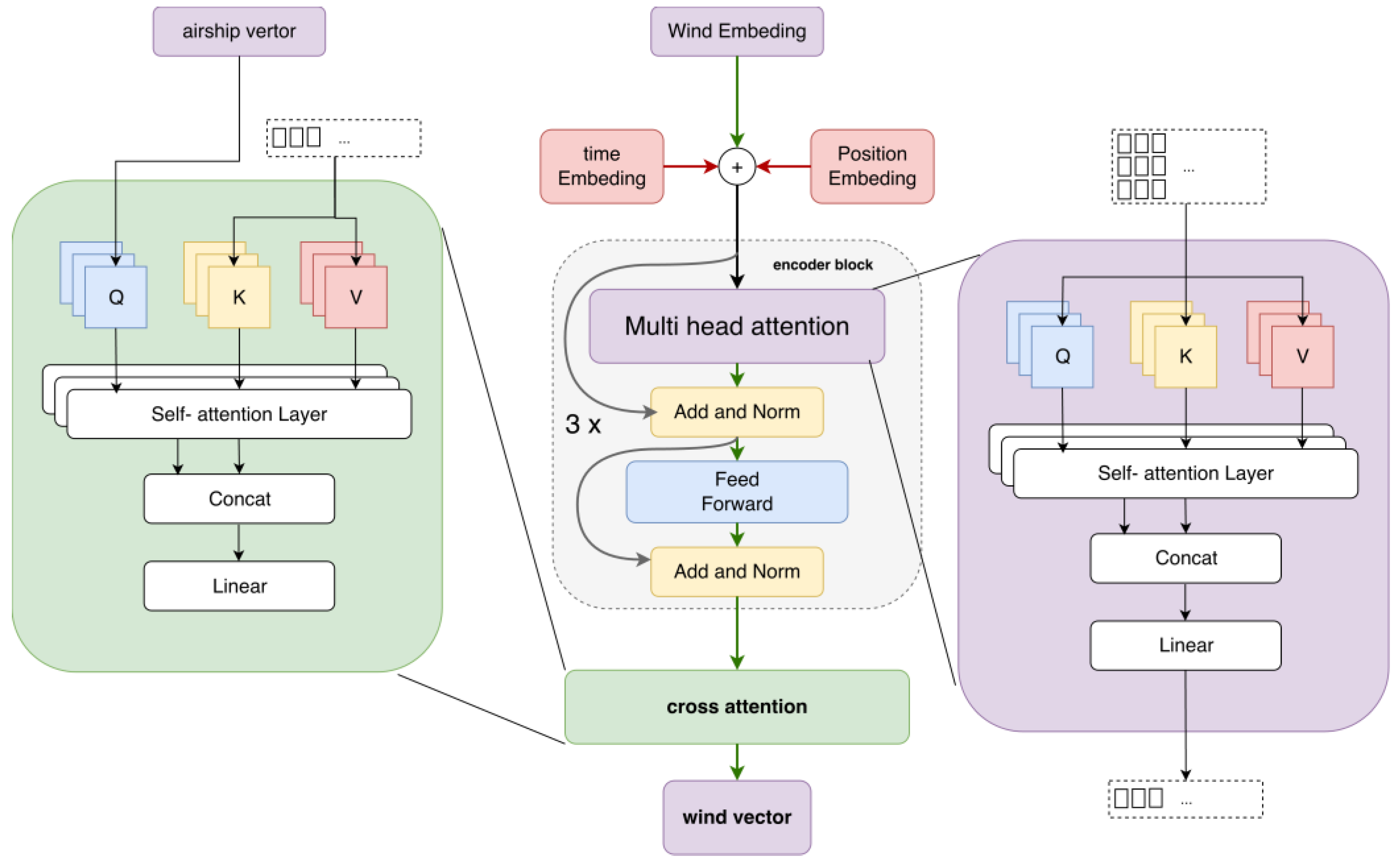
where $N=T\times H$ is the total number of spatio-temporal tokens and $d$ is the feature dimension. The encoder is composed of $L$ stacked Transformer encoder blocks; each block contains a multi-head self-attention (MHSA) sub-layer and a feed-forward network (FFN) sub-layer, with residual connections and layer normalization applied after each sub-layer to improve training stability and representational capacity. The architecture of the Transformer encoder is shown in Figure 4.

For the $l$-th encoder layer, the self-attention computation, illustrated in Figure 4, can be expressed as

$$\begin{array}{c}{\tilde{X}}^l=\mathrm{M}\mathrm{H}\mathrm{S}\mathrm{A}\left(\mathrm{L}\mathrm{N}\left(X^{l-1}\right)\right)+X^{l-1},\\ X^l=\mathrm{F}\mathrm{F}\mathrm{N}\left(\mathrm{L}\mathrm{N}\left({\tilde{X}}^l\right)\right)+{\tilde{X}}^l, l=1,2,\cdots ,L.\end{array}$$

(29)

Multi-head self-attention learns the dependencies between wind tokens by running multiple attention heads in parallel over different sub-spaces. For an individual head, the scaled dot-product attention is defined as

$$\mathrm{A}\mathrm{t}\mathrm{t}\mathrm{n}\left(Q,K,V\right)=\mathrm{s}\mathrm{o}\mathrm{f}\mathrm{t}\mathrm{m}\mathrm{a}\mathrm{x}\left({\displaystyle \frac{Q{K}^{\mathrm{\top }}}{\sqrt{d_k}}}\right)V$$

(30)

where $Q=X{W}_Q, K=X{W}_K, \mathrm{a}\mathrm{n}\mathrm{d} V=X{W}_V$ denote the query, key and value matrices, $W_Q, W_K, \mathrm{a}\mathrm{n}\mathrm{d} W_V$ are learnable parameters, and $d_k$ is the dimensionality of the key vectors. Multi-head attention is written as

$$\mathrm{M}\mathrm{H}\mathrm{S}\mathrm{A}\left(X\right)=\mathrm{C}\mathrm{o}\mathrm{n}\mathrm{c}\mathrm{a}\mathrm{t}\left({\mathrm{h}\mathrm{e}\mathrm{a}\mathrm{d}}_1,{\mathrm{h}\mathrm{e}\mathrm{a}\mathrm{d}}_2,\cdots ,{\mathrm{h}\mathrm{e}\mathrm{a}\mathrm{d}}_M\right)W_O$$

(31)

where $M$ is the number of attention heads and $W_O$ is the output projection matrix. This structure allows the model to attend simultaneously, in different representation sub-spaces, to multiple patterns of the future wind, including coordinated variations across altitude layers, wind-speed trends as a function of lead time, and disturbance features induced by local abrupt changes.

Once the contextualized representations of all spatio-temporal tokens have been obtained, applying global average pooling directly would treat the contributions of different time steps and altitude layers uniformly and fail to highlight the wind information most relevant to the current task state. To overcome this, a task-conditioned attention pooling mechanism is introduced at the encoder output, replacing conventional global average pooling. Specifically, let the output of the last encoder layer be

$$H=\left[h_1,h_2,\cdots ,h_N\right]\in {\mathbb{R}}^{N\times d}$$

(32)

where each $h_i$ is the contextualized wind feature corresponding to a spatio-temporal location. A task query vector is generated from the current airship state vector $s_{\mathrm{airship} }$ via a multi-layer perceptron:

$$q=f_q\left(s_{\mathrm{airship}}\right)\in {\mathbb{R}}^d$$

(33)

Then, with $q$ as the query and the encoded wind sequence $H$ as both key and value, a single cross-attention pooling step yields a wind representation aligned with the current task state:

$$\begin{array}{c}{\alpha }_i={\displaystyle \frac{\mathrm{e}\mathrm{x}\mathrm{p}\left(q^{\mathrm{\top }}{W}_k{h}_i/\sqrt{d}\right)}{{\sum }_{j=1}^N \mathrm{e}\mathrm{x}\mathrm{p}\left(q^{\mathrm{\top }}{W}_k{h}_j/\sqrt{d}\right)}},i=1,2,\cdots ,N\\ z_{\mathrm{wind} }={\displaystyle \sum _{i=1}^N} {\alpha }_i{W}_v{h}_i,\end{array}$$

(34)

where $W_k$ and $W_v$ are learnable projection matrices, and $z_{\mathrm{wind} }\in {\mathbb{R}}^d$ is the resulting wind latent representation. This mechanism enables the model to adaptively select, conditioned on the airship’s current position, target information, remaining energy and motion state, the wind information at different future time steps and altitude layers that is most critical to the current decision, rather than uniformly aggregating all wind tokens.

3.5. Wind-Aware Actor–Critic Coupling and Reinforcement-Learning Optimization

To deeply couple future-wind perception with reinforcement-learning control, an integrated actor–critic architecture is built around a shared wind encoder. The Transformer-based wind encoder serves as the core perception module as follows: it compresses the structural information of the next 12 h of forecast wind into a task-relevant latent representation, which, together with the airship’s current state, is fed into both the policy network and the value network, enabling coordinated optimization of perception and decision-making.

Architecturally, the policy network (actor) and the value network (critic) share the same Transformer wind encoder, ensuring a consistent understanding of the spatio-temporal environmental structure and improving parameter efficiency. To further sharpen policy optimization and value estimation, the actor and the critic are equipped with their own task-conditioned pooling heads and downstream multi-layer perceptron branches. Specifically, given the same set of wind-encoding outputs $H_t$, the actor and the critic generate their respective query vectors from the current airship state:

$$q_t^{\pi }=f_q^{\pi }\left(s_{\mathrm{airship},t}\right),q_t^V=f_q^V\left(s_{\mathrm{airship},t}\right)$$

(35)

and obtain the wind representations corresponding to the policy and value branches via cross-attention:

$$z_{\mathrm{wind},t}^{\pi }=\mathrm{C}\mathrm{r}\mathrm{o}\mathrm{s}\mathrm{s}\mathrm{A}\mathrm{t}\mathrm{t}\mathrm{n}\left(q_t^{\pi },H_t,H_t\right),z_{\mathrm{wind},t}^V=\mathrm{C}\mathrm{r}\mathrm{o}\mathrm{s}\mathrm{s}\mathrm{A}\mathrm{t}\mathrm{t}\mathrm{n}\left(q_t^V,H_t,H_t\right)$$

(36)

leading to the policy and value network inputs

$${\widehat{s}}_t^{\pi }=\left[s_{\mathrm{airship},t};z_{\mathrm{wind},t}^{\pi }\right],{\widehat{s}}_t^V=\left[s_{\mathrm{airship},t};z_{\mathrm{wind},t}^V\right]$$

(37)

This design allows the actor to focus on wind regions and time periods directly related to action selection, while the critic concentrates on the key environmental factors that affect long-term cumulative return, thereby improving the expressive power of each network for its respective task.

For the policy network, because the airship control task studied here lies in a continuous action space, with the action vector composed of propulsion speed, heading angle and vertical speed, the actor is implemented as a multi-layer perceptron that outputs the parameters of a continuous action distribution. Denoting the policy network as ${\pi }_{\theta }$, for a state ${\widehat{s}}_t^{\pi }$ the network outputs the mean and standard-deviation vectors of a Gaussian policy:

$${\mu }_t=f_{\mu }\left({\widehat{s}}_t^{\pi }\right),\mathrm{l}\mathrm{o}\mathrm{g}{\sigma }_t=f_{\sigma }\left({\widehat{s}}_t^{\pi }\right)$$

(38)

from which the continuous action policy distribution is defined as

$$a_t\sim {\pi }_{\theta }\left(a_t\mid {\widehat{s}}_t^{\pi }\right)=\mathcal{N}\left({\mu }_t,\mathrm{d}\mathrm{i}\mathrm{a}\mathrm{g}\left({\sigma }_t^2\right)\right)$$

(39)

where $f_{\mu }(\cdot )$ and $f_{\sigma }(\cdot )$ are implemented as multi-layer fully connected networks whose outputs correspond to the mean and standard-deviation parameters of each action dimension. To ensure that the actions satisfy the airship’s physical constraints, sampled actions are further mapped or clipped to the predefined action ranges.

The value network is implemented as another multi-layer perceptron that takes ${\widehat{s}}_t^V$ as input and outputs the state-value estimate:

$$V_{\varphi }\left({\widehat{s}}_t^V\right)\in \mathbb{R}$$

(40)

where $\varphi$ denotes the parameters of the value network. The value function evaluates the long-term return associated with the augmented state and provides the baseline for advantage estimation and policy updates within PPO.

3.6. Continuous Action Space and Physical Constraints

The action space $\mathcal{A}$ comprises the executable continuous control commands. To enable fine-grained control of the airship in complex wind fields while preserving the convergence and efficiency of reinforcement-learning policy optimization, an action space based on continuous control variables is designed. The action vector at each time step is defined as

$$a_t=\left[V_{\mathrm{t}},\theta ,v_z\right]$$

(41)

where $V_{\mathrm{t}}$ is the horizontal propulsion speed relative to the airflow, $\theta$ is the heading angle relative to the global coordinate system, and $v_z$ is the vertical heave speed. This design fully covers the three-dimensional control degrees of freedom of airship and supports adaptive path adjustment in dynamic environments.

Because the airship is characterized by limited thrust, large inertia and weak maneuverability, abrupt high-frequency action changes are not feasible in actual flight. Several dynamic constraints are therefore imposed on the action space to ensure that the resulting control policies are physically feasible and operationally practical.

In Equation (42), the heading-rate bound is expressed in rad/s, the horizontal-airspeed rate bound in m/s², and the vertical-acceleration bound in m/s². These limits are used to approximate the finite yawing, propulsion and buoyancy/ballonet response capability of a large stratospheric airship. They also prevent the learned policy from exploiting unrealistically abrupt speed or altitude changes that would be infeasible for a high-inertia lighter-than-air vehicle.

$$\left\{\begin{array}{c}-0.02<{\displaystyle \frac{d\mathsf{\theta }}{dt}}<0.02\\ -0.02<{\displaystyle \frac{d{V}_t}{dt}}<0.02\\ -0.001<{\displaystyle \frac{d{V}_{\mathrm{z}}}{dt}}<0.001\end{array}\right.$$

(42)

The continuous action space not only spans the airship’s three-dimensional control degrees of freedom, but also guides the policy, via rate and acceleration constraints, to generate physically feasible and dynamically smooth control sequences. This design provides a structural foundation for stable training and reliable generalization of the reinforcement-learning policy in complex wind fields.

3.7. Reward-Function Design

Within a reinforcement-learning framework, the reward function is the core driver of agent learning: it defines the feedback signal received after taking a specific action and directly determines the optimization direction and convergence behavior of the policy. For the airship path-planning task in wind environments, a well-designed reward function should not only encourage efficient motion towards the target but also account jointly for energy consumption and safety.

Accordingly, a multi-component weighted reward is constructed that jointly models, on a per-step basis, target attainment efficiency, propulsion energy cost, safety boundaries and trajectory smoothness. Its mathematical form is

$$R\left(s_t,a_t\right)=R_{goal}+R_{progress}+R_{energy}+R_{penalty}$$

(43)

Target station-keeping reward. The target reward provides continuous positive reinforcement when the airship is successfully held inside the prescribed region:

$$R_{goal}=\left\{\begin{array}{ll}{R}_{success}& if ‖p_t-p_{goal}‖<\epsilon \\ 0& else\end{array}\right.$$

(44)

where $p_t=\left(x_t,y_t\right)$ denotes the current position, $p_{\mathrm{goal}}=\left(x_{\mathrm{goal}},y_{\mathrm{goal}}\right)$ is the target position, and $\epsilon$ defines the acceptable target tolerance, taken as 40 km in this work.

Progress reward. When the airship lies outside the station-keeping region, this term encourages effective motion towards the target:

$$R_{progress}=\alpha \cdot \left(‖p_t-p_{goal}‖-‖p_{t+1}-p_{goal}‖\right)$$

(45)

where $\alpha >0$ is a scaling factor that balances the magnitude of the progress reward against the other reward components.

The reward coefficients were fixed for all compared methods so that the comparison is determined by the state representation and policy architecture rather than by method-specific reward tuning. In the experiments, the target-success reward is set to R_success = 1, the progress coefficient is set to alpha = 0.1, the boundary-violation coefficient is set to gamma_boundary = 2, and the trajectory-smoothness coefficient is set to gamma_stability = 0.5. These values keep the dense progress reward on the same order as the target reward while assigning a larger cost to safety-boundary violations.

Energy-consumption penalty. As the airship consumes electrical energy in flight and replenishes it via solar charging, the battery state of charge varies dynamically. To ensure that the airship retains sufficient energy to keep avionics operational and to handle contingencies, a minimum energy reserve must be maintained. A penalty is therefore imposed when the battery energy becomes too low:

$$R_{energy}=\left\{\begin{array}{c}0, {\displaystyle \frac{E_{t }}{E_{\mathrm{m}\mathrm{a}\mathrm{x}}}}>0.4\\ -2, {\displaystyle \frac{E_{t }}{E_{\mathrm{m}\mathrm{a}\mathrm{x}}}}<0.4\end{array}\right.$$

(46)

where $E_{t }$ is the current battery energy state and $E_{\mathrm{m}\mathrm{a}\mathrm{x}}$ is the maximum battery energy capacity.

The state-of-charge threshold E_t/E_max = 0.4 is used as an engineering reserve rather than as a hard physical failure boundary. It preserves sufficient energy margin for avionics, nighttime operation and unexpected headwind periods. The penalty value −2 is intentionally larger than the unit target reward so that the policy does not trade long-term energy safety for short-term position keeping. A complete sensitivity analysis of this threshold and penalty magnitude is reserved for future work, and the present manuscript avoids claiming that these values are universally optimal.

Safety and constraint penalty. To ensure safe operation, penalty terms are included for boundary violations and trajectory non-smoothness:

$$R_{penalty}=-{\gamma }_{boundary}\cdot I_{boundary}-{\gamma }_{stability}\cdot f_{stability}$$

(47)

where $I_{boundary}$ is the indicator function of boundary-violation events, and $f_{\mathrm{stability} }$ penalizes excessive angular rates or accelerations that may threaten the airship’s stability.

4. Experiments

To systematically evaluate the station-keeping path-planning performance of the proposed STF-RL method in complex wind environments, experiments are conducted along the following three axes: training convergence, overall performance and the effectiveness of key modules. All methods are trained and tested under the same airship dynamics, wind-disturbance model, energy-constraint model and task settings to ensure a fair comparison.

4.1. Experimental Setup

A three-dimensional high-altitude station-keeping simulation environment is built on the basis of reanalysis wind data to emulate the long-term regional station-keeping of a stratospheric airship under complex dynamic winds and energy constraints. The wind data have a fixed temporal and spatial resolution and cover multiple discrete flight layers within the airship’s reachable altitude range. At each decision step, the agent obtains not only the airship’s current motion state, energy state and target-position information, but also forecast winds at multiple altitude layers over a finite future horizon. It should be noted that the future-wind data used in this work are supplied by an external forecasting system; the model itself does not perform wind forecasting but uses the Transformer module to extract spatio-temporal features that yield a latent environmental representation aligned with the current decision, consistent with the methodology in earlier sections.

To enhance environmental stochasticity and improve the practical adaptability of the policy, a zero-mean Gaussian disturbance is superimposed on the baseline wind field, emulating forecast errors and small-scale wind fluctuations. The airship motion follows the simplified three-dimensional kinematic model established earlier, with control variables comprising propulsion speed, heading angle and vertical speed. A solar charging–discharging dynamic model is also incorporated, requiring the agent to ensure long-term energy sustainability while maintaining regional station-keeping. The task is therefore not a simple target-tracking problem, but a multi-objective decision-making problem involving spatial station-keeping, energy management and safety constraints.

Regarding task generation, at the beginning of each episode the airship’s initial position, initial altitude, target-region center and start time are randomly sampled to prevent the policy from overfitting to fixed task patterns. The target station-keeping region is defined as a circular area of radius R centered on the target. Each episode lasts for a fixed duration T, during which the agent is required to maintain the airship in the vicinity of the target region by actively adjusting flight speed, heading and altitude. The main parameters of the simulation environment and task configuration are summarized in

Table 1. Simulation environment and task-setting parameters.

Parameter	Value	Description
Wind-data source	ERA5	Used to construct the 3D station-keeping simulation
Temporal resolution	1 h	Wind-field temporal sampling interval
Spatial resolution	0.25° × 0.25°	Horizontal grid resolution
Altitude range	[18, 22] km	Reachable flight-altitude range of the airship
Number of discrete altitude layers	21	Vertical sampling layers
Future forecast horizon	12 h	Future-wind window used as policy input
Decision time step	300 s	Agent action-update interval
Episode duration	72 h	Duration of each episode
Target station-keeping radius	40 km	Threshold for target-region attainment
Wind-disturbance distribution	Gaussian	Used to emulate forecast errors and random disturbances
Propulsion-speed range	[0, 30] m/s	Action-space constraint
Heading-angle range	[−π, π]	Action-space constraint
Vertical-speed range	[−1, 1] m/s	Action-space constraint
Representative envelope shape	Streamlined prolate-spheroid-like hull	Physical scale used to interpret the mission-level parameters
Representative envelope length	150 m	Geometry scale for the case study
Representative maximum diameter	40 m	Geometry scale for the case study
Approximate envelope volume	1.2 × 105 m3	Buoyancy/size scale of the representative vehicle
Frontal reference area	1.26 × 103 m2	Approximate πD2/4 area used as a fluid-dynamic scale

.

To verify the effectiveness of the proposed method, three approaches are compared. The first is standard PPO, which uses only the airship’s current state as input and does not explicitly exploit future-wind information; it is a typical reactive reinforcement-learning baseline. The second is LSTM-PPO, which encodes the future-wind sequence with an LSTM and concatenates the result with the current airship state before feeding it to the policy network; it is used to compare classical sequence models against the proposed method. The third is the proposed STF-RL, which models future multi-altitude winds with a Transformer encoder equipped with the time–height dual positional encoding, generates a latent environmental representation through task-conditioned pooling—drawing on design ideas from multivariate time-series representation learning and long-sequence forecasting—and feeds the result into an actor–critic network for decision-making and value estimation.

All methods adopt the same number of training epochs, the same reward-function structure and the same main reinforcement-learning hyperparameters. Apart from the wind-encoding scheme, all settings are kept identical. The simulation parameters and training hyperparameters are listed in Table 1 and

Table 2. Main training hyperparameters.

Parameter	Value
Optimizer	Adam
Learning rate	1 × 10−5
Batch size	64
Discount factor	0.99
GAE parameter	0.95
PPO clipping parameter	0.2
Entropy regularization coefficient	0.01
Number of parallel environments	10
Number of Transformer encoder layers	3
Number of attention heads	4
Hidden dimension	256
Feed-forward dimension	256
Dropout	0.1
Target reward R_success	1
Progress coefficient alpha	0.1
SOC safety threshold	0.4
Low-energy penalty	−2
Boundary penalty coefficient gamma_boundary	2
Stability penalty coefficient gamma_stability	0.5
Evaluation seeds	multiple seeds, averaged

, respectively.

Each test scenario was evaluated using multiple random seeds and randomized initial conditions, and the values reported in the comparison tables are the corresponding averages. This setting reduces dependence on a single rollout and makes the reported cross-seasonal comparison more representative of the policy behavior under randomized initial position, altitude, target-region center and start time.

The parameter choices in Table 1 are selected to match the spatial and temporal scale of long-endurance stratospheric station-keeping. ERA5 is used as the background atmospheric dataset because it provides globally consistent reanalysis winds; its 1 h temporal resolution and 0.25 deg × 0.25 deg horizontal grid determine the wind-field sampling scale. The 18–22 km altitude interval represents the typical operating range considered for stratospheric airships, and 21 discrete layers provide 200 m vertical spacing for altitude-selection decisions. The 12 h wind window gives the policy a sub-daily foresight horizon while keeping the Transformer input size tractable. The 300 s decision step is chosen for mission-level control, where the agent updates guidance commands more slowly than the low-level attitude controller.

To give the simulation a concrete physical scale, the mission is interpreted using a representative streamlined stratospheric airship geometry as follows: an axisymmetric prolate-spheroid-like envelope with length 150 m, maximum diameter 40 m, approximate volume 1.2 × 10⁵ m³ and frontal reference area about 1.26 × 10³ m². The present study does not solve the geometry-dependent aerodynamic force and moment equations directly; instead, these physical dimensions motivate the bounded airspeed, vertical-rate, action-smoothness and propulsion-power settings used by the mission-level planning environment. This clarification connects the abstract control model to a plausible vehicle scale while preserving the paper’s focus on foresighted path-planning policy design.

To evaluate the performance of different methods comprehensively, the following three quantitative metrics are adopted: the station-keeping ratio (SKR), the mean station-keeping error (MSER), and the minimum state of charge (Min-SOC). These are supplemented by a qualitative analysis of two-dimensional trajectories, energy time histories and key control-state curves under typical test scenarios. SKR measures the fraction of time the airship spends inside the target region and is the core metric for long-term station-keeping capability; MSER measures the average distance between the airship and the center of the target region and reflects path-control accuracy; Min-SOC reflects the safety margin of battery energy during the mission. These three metrics correspond to station-keeping efficiency, control accuracy and energy safety, respectively, and together provide a comprehensive evaluation of the path-planning policy.

4.2. Training-Convergence Analysis

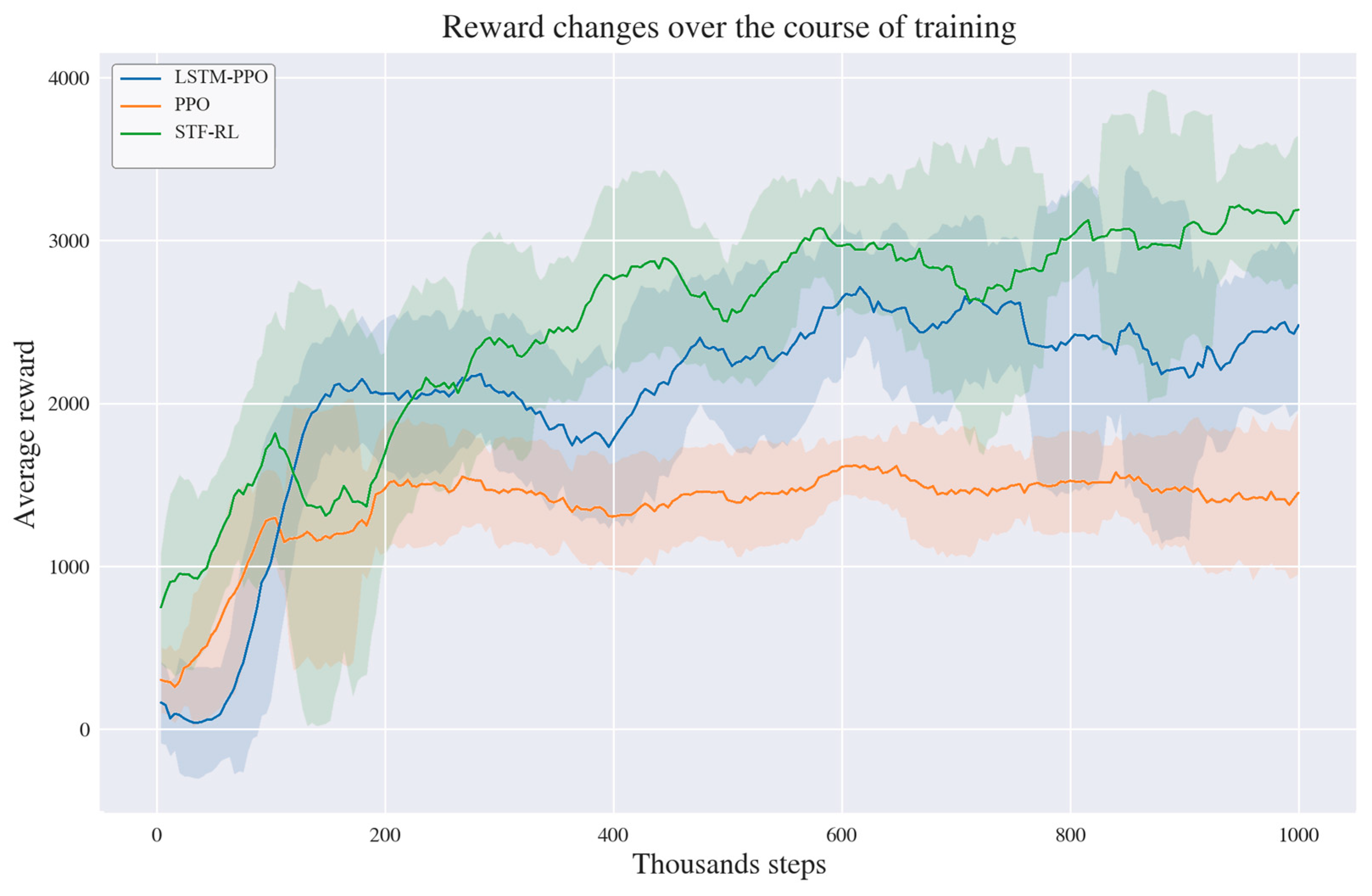
To verify the optimizability and stability of the proposed method during long-horizon reinforcement-learning training, Figure 5 reports the average episode return versus environment-interaction steps for each method. The horizontal axis denotes the number of environment steps, and the vertical axis denotes the average cumulative return across parallel environments; the shaded regions indicate the variance.

As shown in Figure 5, all three methods undergo a clear exploration phase early in training, with low and highly variable returns. PPO escapes the random-policy regime relatively quickly but enters a plateau early on, with limited subsequent improvement, indicating that a reactive policy relying solely on current observations cannot consistently meet the long-horizon decision-making requirements of strongly time-varying winds. LSTM-PPO exhibits a faster mid-training increase in return, suggesting that incorporating future-wind sequences improves sample efficiency and enhances foresight; however, its curve still shows pronounced retracement and oscillation in the middle and late stages, implying that purely temporal sequence modeling is insufficient to stably capture the structural differences between altitude layers. By contrast, STF-RL maintains the highest return level after the early phase and exhibits relatively narrower late-stage variability. This indicates that explicitly modeling both the temporal evolution and the vertical-layer structure of the future wind not only improves the final policy performance but also enhances optimization stability during training, allowing the agent to more readily acquire stable control patterns aligned with the long-term station-keeping objective.

4.3. Comparative Experiments

To systematically evaluate the proposed method’s overall performance in complex time-varying winds, cross-scenario validation is performed under typical wind backgrounds for the four seasons, examining the generalization and robustness of each method when the environmental distribution changes. The corresponding quantitative results are summarized in

Table 3. Performance comparison of the different methods on the comprehensive test set and the cross-seasonal test set. The arrows indicate the preferred direction of each metric: higher is better for SKR and Min-SOC, and lower is better for MSER. Bold values indicate the best result for each metric.

Test Scenario	Method	SKR (%) ↑	MSER (km) ↓	Min-SOC (%) ↑
January	PPO	86.53	14.41	23.61
	LSTM-PPO	97.73	12.43	47.55
	STF-RL	97.96	10.32	54.53
April	PPO	84.79	15.57	15.19
	LSTM-PPO	97.43	7.43	63.90
	STF-RL	98.02	8.69	66.81
July	PPO	85.24	12.66	43.26
	LSTM-PPO	98.13	10.02	59.41
	STF-RL	98.45	9.41	68.37
October	PPO	86.14	11.94	38.62
	LSTM-PPO	98.67	10.21	57.46
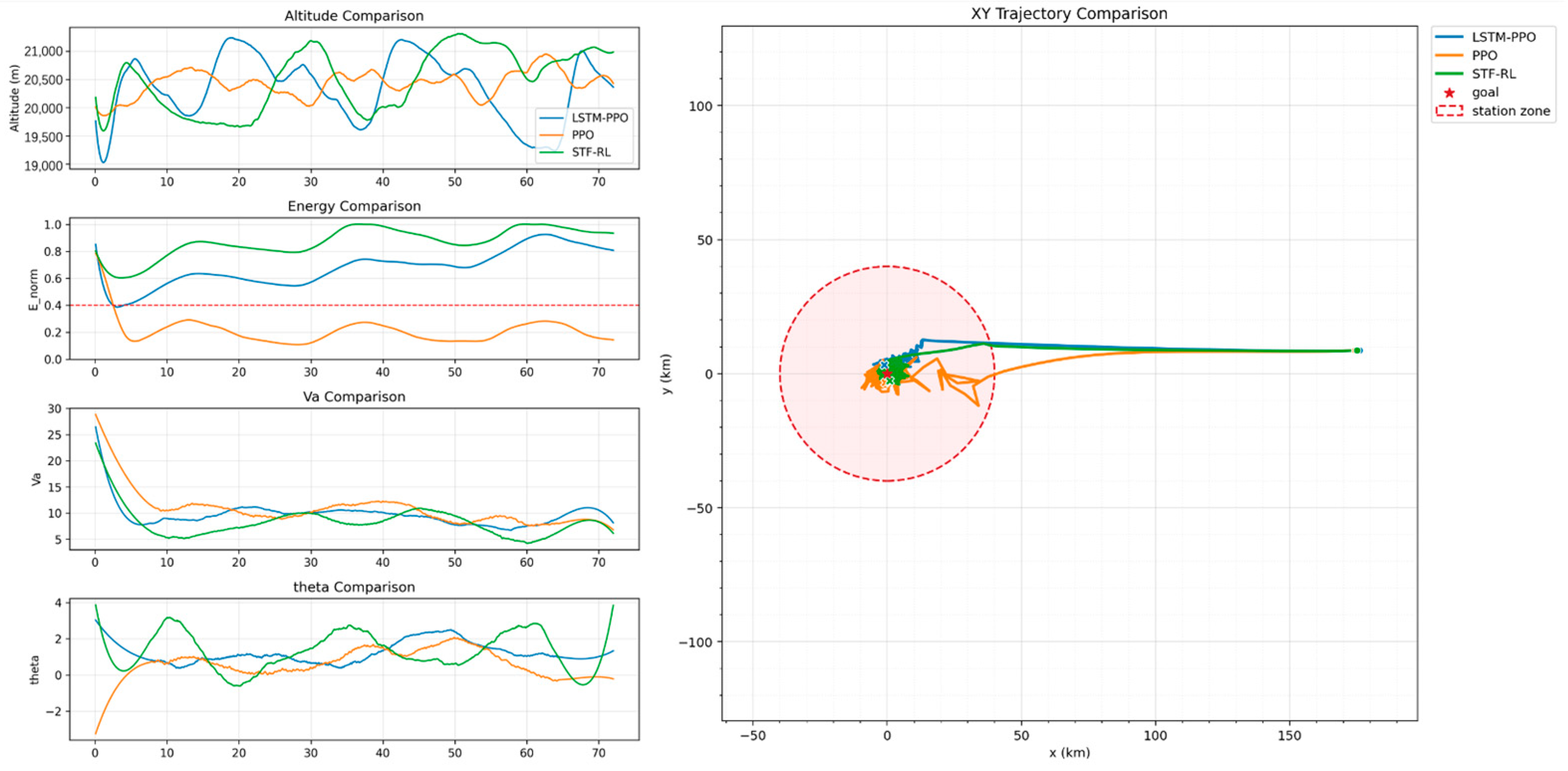
	STF-RL	98.85	10.09	68.08

, while the two-dimensional trajectories and the evolution of key state variables under a representative test scenario are shown in Figure 6.

Figure 6 presents a representative comparative test. All three policies converge from similar initial regions towards the target region, but their convergence behavior and the trajectory shape during station-keeping differ markedly. After approaching the target region, PPO still exhibits noticeable circling and back-and-forth motion near the boundary, with relatively dispersed trajectories, indicating limited efficiency in correcting position deviations under local wind disturbances. LSTM-PPO improves lateral-deviation suppression compared with PPO, but its trajectory cluster remains somewhat extended, suggesting that its motion organization during station-keeping is not yet sufficiently compact. By contrast, STF-RL produces a more concentrated trajectory distribution near the target region, demonstrating that it can sustain station-keeping with lower wasted maneuvering effort and thus achieves higher trajectory-organization efficiency.

The evolution of the key state variables is consistent with the trajectory features above. PPO shows a pronounced energy decline early in the mission and remains at a low level for an extended period afterwards, indicating that this policy tends to use passive corrections to handle environmental disturbances and therefore incurs higher energy consumption. Although LSTM-PPO improves energy maintenance relative to PPO, its altitude, airspeed and attitude angles still show noticeable fluctuations, reflecting limited control smoothness during wind-layer switching and speed regulation. By contrast, STF-RL achieves long-term station-keeping at higher states of charge, with smoother altitude adjustment, speed variation and attitude response overall, indicating that the method exploits favorable wind layers more purposefully and achieves a more coordinated allocation of decisions among environmental perception, trajectory correction and energy management. The performance advantage of STF-RL therefore does not stem from frequent or large-amplitude maneuvering corrections, but from more effective use of the structural information in the wind field and the resulting improvement in control rhythm.

The cross-seasonal tests further confirm the robustness of STF-RL under averaged evaluations over multiple random seeds and randomized initial conditions. From January to October, the seasonal wind fields differ markedly in intensity, direction and inter-layer variability; nevertheless, STF-RL maintains a high average SKR across all scenarios and consistently achieves the highest average Min-SOC. Although STF-RL does not always achieve the absolute best MSER-LSTM-PPO obtains a lower average error in the April scenario, for example, the averaged results indicate that STF-RL provides a better overall trade-off among station-keeping success rate, error control and energy margin. Compared with the baselines, the proposed method is therefore not only competitive on individual metrics, but also more reliable and adaptive across environments, which is of greater practical value for long-term high-altitude station-keeping missions.

4.4. Ablation Study

To further identify the specific contribution of each key design to policy learning and final station-keeping performance, three ablation variants are constructed on the basis of the full model and compared under identical training and test settings. The three variants are: (1) removing the future-wind input and using only the airship’s current state as policy input (without Future Wind); (2) retaining the future-wind input and the Transformer encoder but removing the time–height dual positional encoding (without THDPE); and (3) replacing the task-conditioned cross-attention pooling with simple feature aggregation (without Cross Attention).

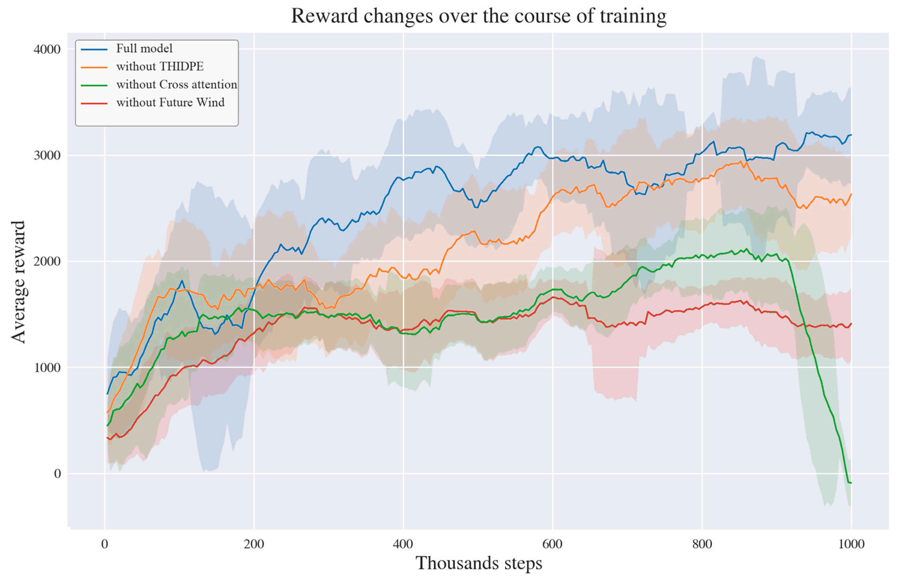
Figure 7 reports the average return during training for the full model and the three ablation variants. The full model exhibits a faster early-training rise in performance and consistently maintains a higher return level in the middle and late stages, showing that the proposed overall architecture not only raises the final performance ceiling but also improves sample efficiency and convergence stability during policy optimization. By contrast, the ablation variants exhibit varying degrees of restricted convergence or training instability, indicating that the modules are not merely additive but jointly support policy representation learning and decision optimization throughout training.

When the future-wind input is removed, the model remains at the lowest return level throughout training; although the curve rises somewhat, the overall improvement is limited and the policy enters a plateau early on. This shows that, when only current-state information is available, the policy struggles to form effective estimates of long-term return and can hardly produce foresighted, high-quality decisions in complex time-varying winds. With the future-wind input retained but THDPE removed, the training curve continues to rise and reaches a relatively high level in the middle and late stages, indicating that future-wind information by itself already provides important support for policy learning; however, the return remains below that of the full model and exhibits more pronounced fluctuations, showing that without temporal- and altitudinal-structure encoding the model cannot organize this future-wind information stably and accurately. When the cross-attention is removed, the model still achieves some return improvement during the early-to-mid stages of training, but suffers a clear performance drop later, with the return curve even collapsing rapidly towards the end. This indicates that this module plays a critical role in stable late-stage convergence as follows: without task-conditioned guidance, the model’s exploitation of future-wind features tends to destabilize as training progresses, leading to policy degradation.

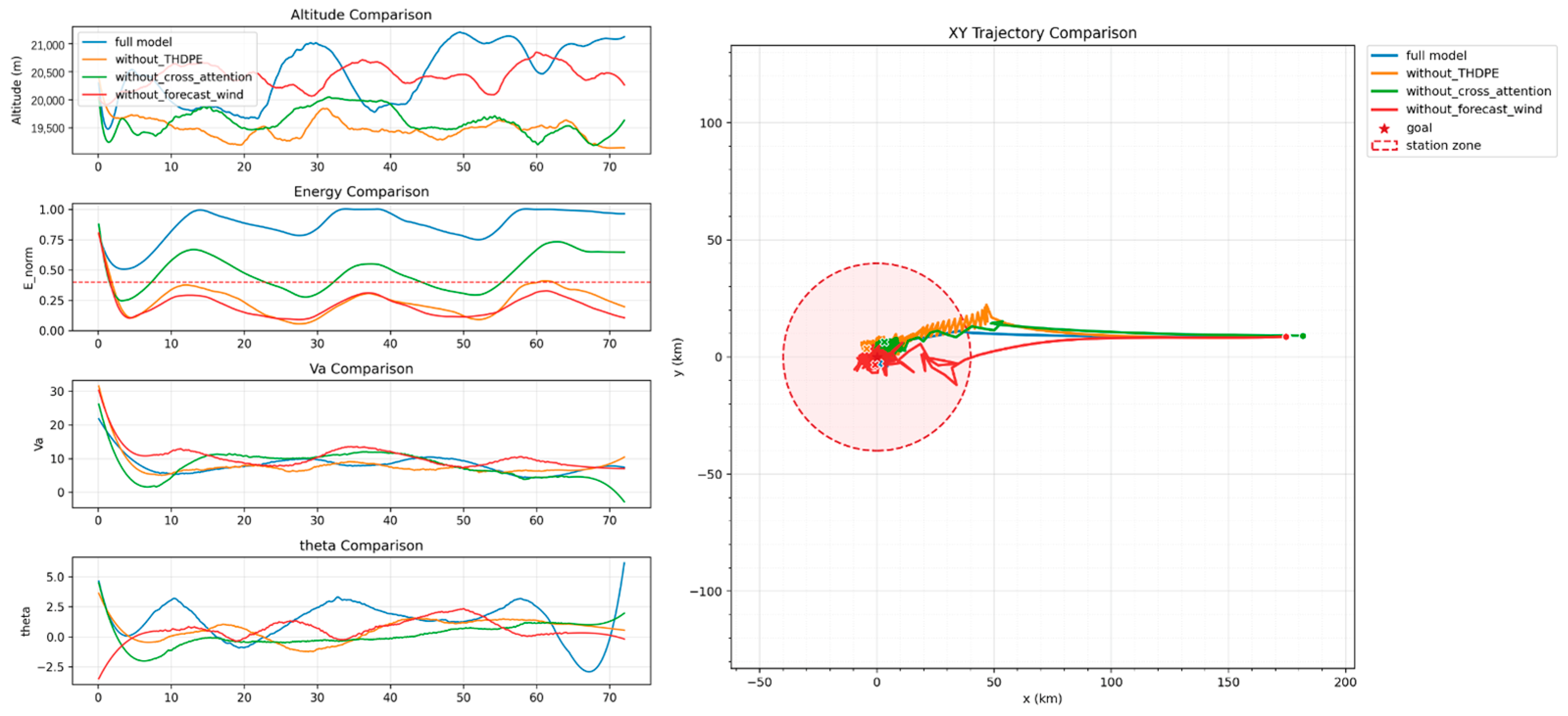
Figure 8 further visualizes the behavioral differences among the ablation variants in terms of trajectories and the evolution of key state variables. Consistent with the training curves, the full model exhibits the most rational trajectory organization and the smoothest state regulation in the representative test scenario. Its two-dimensional trajectory shows that the airship rapidly approaches the target region and then forms a more compact local trajectory distribution near it, indicating that the policy retains good position-constraint capability after reaching the target. At the same time, the evolution of altitude, energy, airspeed and attitude angles is generally smooth, without abrupt high-frequency oscillations, showing that the model achieves good coordination among wind-layer switching, energy maintenance and position correction.

By contrast, the degradation of without-Future-Wind is the most pronounced. After approaching the target, its trajectories remain markedly dispersed and exhibit persistent drift and repeated corrections, failing to form a stable station-keeping structure; the state curves further show a rapid drop in energy that remains low for long periods, while altitude and speed regulation lack a stable rhythm. This indicates that, in the absence of an environmental prior, the policy relies mainly on passive correction rather than foresighted planning, leading to loose trajectories and insufficient energy margin. Without-THDPE can enter the target region and maintain basic station-keeping, but its trajectory cluster is clearly less compact and at certain stages exhibits a mismatch between altitude adjustment and energy variation. This shows that the issue is not whether future-wind information is available, but whether the model can correctly parse its temporal order and vertical stratification: without structural encoding, the policy struggles to consistently exploit favorable wind layers, leading to station-keeping behavior that is “reachable but suboptimal”. Without-Cross-Attention shows reduced stability as follows: its trajectories near the target exhibit more pronounced local oscillation, and the state variables, particularly speed and attitude angles, fluctuate more strongly. Together with the late-stage decline in return, this indicates that, although environmental information is still available as input, the model lacks an effective filtering mechanism, leading to temporally inconsistent decisions and consequent local oscillations and performance degradation.

Table 4. Ablation results. The arrows indicate the preferred direction of each metric: higher is better for SKR and Min-SOC, and lower is better for MSER. Bold values indicate the best result for each metric.

Model Variant	SKR ↑	MSER (km) ↓	Min-SOC ↑
without Future Wind	85.32	15.83	21.71
without THDPE	97.04	10.40	32.57
without Cross attention	91.02	14.33	48.72
Full model	98.42	9.41	68.21

reports the quantitative comparison of the different model variants in terms of the station-keeping ratio (SKR), the mean station-keeping error (MSER) and the minimum state of charge (Min-SOC). The full model achieves the best performance on all three metrics, indicating that the three key modules jointly enhance station-keeping effectiveness, position-control accuracy and energy safety margin, rather than acting on a single objective only.

Without-Future-Wind exhibits the most pronounced performance degradation, with SKR dropping to 85.32%, MSER rising to 15.83 km and Min-SOC reaching only 21.71%. This indicates that, without future environmental information, the model not only struggles to maintain stable station-keeping but also pays a higher energy cost during the mission, with the overall policy lacking foresight and energy coordination. Without-THDPE retains an SKR close to that of the full model (97.04%), but MSER rises to 10.40 km and Min-SOC drops markedly to 32.57%. This indicates that this module mainly affects the fine-grained exploitation of wind information as follows: although the model can still complete the task, it cannot achieve a good balance between error control and energy management. Without-Cross-Attention yields SKR and MSER of 91.02% and 14.33 km, respectively, both clearly inferior to those of the full model, while Min-SOC is 48.72%. Together with the trajectory dispersion and state oscillation, this indicates that the module mainly affects decision stability as follows: without task-conditioned constraints, the model cannot consistently extract the key environmental information, which reduces overall control accuracy.

Combining the results in Figure 7 and Figure 8 and Table 4, it can be seen that the three key modules of the proposed model correspond to three core capability dimensions of long-term station-keeping decision-making as follows: foresighted environmental modeling, parsing of the spatio-temporal structure of the wind field, and task-relevant information filtering with stable decision-making. These three dimensions exhibit a consistent pattern across training dynamics, behavioral manifestations and final performance metrics, forming a complete and mutually dependent information-processing pipeline.

More specifically, the future-wind input mainly determines whether the policy is capable of foresighted environmental modeling; its absence directly limits the optimization of long-term return, manifested as restricted training convergence, loose trajectories and reduced energy efficiency. The time–height dual positional encoding further structures the wind information, enabling the model to distinguish wind features at different time steps and altitude layers and thus supporting finer wind-layer selection and trajectory organization; its absence does not preclude task feasibility but markedly weakens error control and energy management. The cross-attention mechanism builds on these foundations by introducing task-conditioned constraints, enabling the dynamic filtering and aggregation of multi-scale wind representations and thereby improving decision consistency and stability; once it is removed, although environmental information is still available as input, the policy is prone to degradation and control oscillations in long-term decision-making.

Therefore, the performance advantage of the full model does not stem from local improvements of any single module, but from the synergy of a hierarchical information-processing pipeline. The result indicates that, under complex time-varying winds, long-term station-keeping is essentially a problem of multi-scale environmental perception coupled with decision-making, and that relying solely on instantaneous state feedback or on a single time-series model is insufficient to fully exploit the decision value of environmental information. By contrast, jointly modeling future environmental information, structured representations and a task-driven information-filtering mechanism markedly improves the stability, energy efficiency and long-term reliability of the policy.

5. Limitations and Future Work

This work focuses on the decision-making layer of long-duration station-keeping and therefore retains several modeling assumptions. First, the airship is represented by a mission-level kinematic model rather than a full six-degree-of-freedom aerodynamic model. This abstraction is appropriate for evaluating long-horizon planning behavior and wind-layer selection, but it does not fully capture attitude dynamics, envelope deformation, actuator transients, detailed aerodynamic coefficients or closed-loop flight-control effects. Second, the wind-disturbance term is modeled as a simplified stochastic perturbation added to the reanalysis/forecast wind field. In real deployments, forecast errors are altitude-, season- and region-dependent, and can include structured biases that are not represented by the present disturbance model.

The energy model and reward design also impose controlled assumptions. The current simulation captures the main coupling among propulsion demand, solar input and battery SOC, but it does not model all payload modes, thermal-management loads, battery aging or emergency operational constraints. Moreover, although the SOC threshold and low-energy penalty are selected according to engineering interpretation and reported explicitly, a systematic sensitivity sweep over these reward coefficients has not yet been conducted. The reported results should therefore be interpreted as evidence that the proposed representation and policy framework are effective under the specified protocol, rather than as proof of universal optimality of the selected reward parameters.

Future work will extend the framework in four directions. First, robust decision-making under forecast uncertainty will be studied by incorporating ensemble forecasts, altitude-dependent error models and risk-sensitive objectives. Second, higher-fidelity airship dynamics, propulsion constraints and energy-system models will be coupled with the planner to improve engineering validity. Third, the evaluation will be expanded to broader mission regions, forecast horizons, disturbance intensities and task scales, together with threshold-sensitivity analysis and hardware-in-the-loop or real-flight validation. Fourth, future planning frameworks should explicitly include operational and regulatory constraints, such as airspace separation, communication-link availability, spectrum coordination and mission-approval requirements, so that algorithmic station-keeping can better support certifiable and standardized stratospheric-platform operations.

6. Conclusions and Discussion

This paper addresses the long-term station-keeping problem of stratospheric airships in complex time-varying winds and proposes an altitude-changing path-planning method that integrates spatio-temporal future-wind encoding with reinforcement-learning decision-making. The method incorporates multi-step, multi-altitude future winds provided by an external numerical forecasting system into the decision process, uses a Transformer encoder to extract environmental features relevant to the current task, and combines them with the airship’s current position, flight state and energy information to form an augmented state input. PPO is then employed for continuous-control policy optimization. A continuous action space comprising propulsion speed, heading angle and vertical speed is designed, allowing the policy to actively select more favorable wind layers via adaptive altitude adjustment and thereby balance station-keeping and energy constraints. Experimental results show that the proposed method achieves stable regional station-keeping under typical seasonal wind conditions and exhibits superior trajectory control and energy management in comparative experiments, demonstrating that explicitly exploiting future-wind trends can improve the long-term decision performance of an airship in dynamic environments.

Overall, the results indicate that long-term stratospheric airship station-keeping is not only a trajectory-control problem, but also a spatio-temporal environmental-perception and energy-coordination problem. By introducing future-wind representation learning into the reinforcement-learning policy, the proposed framework provides a practical basis for more reliable autonomous planning under dynamic winds. The main modeling assumptions and future extensions are summarized separately in Section 5.