Dynamic Trajectory Planning for Autonomous Parafoil Homing Under Wind Disturbances

Abstract

The parafoil is highly susceptible to deviations from its reference trajectory under wind disturbances. Given its constrained longitudinal control authority, it has limited capability to correct these deviations and regain the intended glide path. To overcome this limitation, we propose a dynamic planning framework based on a layered homing strategy. The airdrop mission trajectory is initially designed as a traditional multi-segment path. To approximate non-uniform glide characteristics under wind disturbances, this planning problem incorporates a predicted wind model as an external input. Node parameters of the segmented trajectory are then solved using an improved grey wolf optimizer (IGWO). By tracking this reference trajectory, the parafoil is guided into the proximity of the target. To ensure landing precision, the terminal phase is formulated and discretized using an adaptive pseudo-spectral method (APSM). The online planner computes a real-time trajectory to account for actual motion characteristics. This dynamic replanning (DRP) compensates for deviations caused by model mismatches and external disturbances. The proposed homing method is statistically verified via extensive Monte Carlo simulations under different wind conditions. Finally, the airdrop experiment is conducted to validate the DRP method.

1. Introduction

Parafoils are typically used for long-distance delivery from an airdrop vehicle due to their superior gliding performance [1,2,3]. The ram-air parafoil achieves sustained unpowered flight through its stable airfoil shape when inflated. Driven by its extended glide range and greater payload capacity, the demand for precise autonomous airdrop systems based on this technology has grown markedly in recent years.

However, the limited glide ratio of the unpowered parafoil restricts its height adjustment. Its inefficient longitudinal control further dictates that precise trajectory planning is essential for landing accuracy. As a result, the reference trajectory must satisfy the inherent gliding characteristics in both horizontal and vertical dimensions. Previous studies have proposed various path planning methods for parafoils, such as the rapidly exploring random tree (RRT) algorithm [4,5], smooth curve-based methods [6,7,8], and methods formulated as optimal control problems [9,10]. RRT can rapidly generate a path in complex environments, and is widely used in aviation guidance due to its rapid calculation capacity. However, as the resulting path is typically zigzag and does not account for continuous kinematic constraints, a subsequent smoothing process is required for effective guidance.

Smooth curve-based methods, notably Bézier and Dubins curves, offer a distinct advantage over RRT by generating trajectories that are inherently continuous and comply with geometric conditions [11,12]. This characteristic makes them particularly suitable for parafoil homing design, as the resulting trajectories are more consistent with flight dynamics. Some studies have introduced the segmented homing method, which guides the parafoil along multiple predetermined geometric segments in sequence [9,13]. A trajectory composed of multiple arc curves and straight lines aligns well with the parafoil turning and gliding maneuvers. The key parameters defining these segments can be obtained to solve an associated planning problem using various algorithms, including the genetic algorithm, the ant colony algorithm, and the gray wolf optimizer [14,15,16]. In addition, trajectory planning formulated as an optimal control problem has been explored to meet various requirements, such as wind resistance and terrain avoidance. The pseudo-spectral method is commonly employed to transcribe the continuous optimization problem into a discrete nonlinear programming problem (NLP) [17,18]. The optimized reference trajectory is capable of closely matching the parafoil gliding characteristics, simultaneously satisfying different objectives, such as minimizing energy assumptions, avoiding obstacles, and enabling an upwind approach. However, this method faces challenges in effectively managing the planning space. Specifically, the presence of height redundancy necessitates extensive horizontal maneuvers to lose height, resulting in a narrow adjustment margin near the terminal target point.

Parafoils are highly sensitive to wind disturbances, which can induce significant trajectory deviations along the wind direction. The effective glide ratio (GR) varies with the relative angle between the wind flow and the parafoil heading [19]. To account for this influence, wind speed is generally estimated as a function of height [20]. Furthermore, environmental wind forecasts can be incorporated a priori to enhance the robustness of trajectory planning [21]. However, effectively incorporating predicted external information to achieve landing remains challenging when dealing with an unknown airdrop area.

The predefined trajectories typical of conventional planning methods are static and lack adaptability to external disturbances. Wind gusts can cause deviations from the reference trajectory during flight. The control authority in the longitudinal/vertical channel is limited for glide slope adjustment when relying solely on symmetric trailing-edge deflection. This limitation can result in landing errors, manifesting as overshooting the target or landing short of it. Various auxiliary measures, such as adjusting the movable center of gravity, altering the canopy incidence angle, and deploying spoilers on the upper surface, have been utilized to enhance control efficiency [22,23,24]. However, these methods often add extra structural weight and increase system complexity. Given this limitation, research into efficient online planning methods is therefore needed to correct trajectory deviations with minimal hardware configuration changes [25]. In related fields, real-time trajectory adjustment methods have been established to enhance the tracking performance of various vehicles, and online optimization techniques are being explored to improve practical applicability [26,27,28]. In parafoil homing, several methods have been proposed to calculate control points online using real-time wind field measurements. During the terminal T-approach phase on Titan, a local grid refinement is employed to enhance computational efficiency [29].

As the major development of a precise airdrop system, Joint Precision Airdrop System (JPADS) provided an error threshold of a landing precision of 100 m under non-ideal conditions [30]. Adopting this as the design objective, this paper proposes a layered homing strategy that integrates pre-planning with DRP. Distinct methods are tailored for each phase to generate trajectories that meet specific requirements. The offline component utilizes multiple-segmented Dubins curves, which incorporate a wind prediction model. An IGWO is employed to obtain highly accurate solutions. For the terminal flight phase, an online RP scheme is implemented to dynamically adjust the path. Based on the APSM, the trajectory planning problem is reformulated from the current flight position to compensate for accumulated tracking errors caused by external disturbances. The main contributions of the paper are summarized as follows:

• The multi-segment Dubins curves are employed to more effectively incorporate the wind model, thereby providing a closer approximation of the homing trajectory of the parafoil in windy conditions. Specifically, wind effects are accounted for to estimate the realistic GR characteristics at each height layer.
• Landing performance in the terminal phase is further improved by a real-time replanning (RP) scheme. This approach reformulates the planning problem for the terminal region through the APSM, where normalization of time and state variables reduces computational costs. The trajectory is adjusted based on the prediction of glide characteristics, reducing tracking errors during the subsequent flight phase.
• A mathematical model of the parafoil system integrated with an autonomous control system is developed based on the line of sight (LOS) guidance and linear active disturbance rejection control (LADRC). Under various wind disturbances, the proposed hybrid planning method is validated by tracking trajectories with this model. Airdrop experiments are conducted to analyze the wind effect and validate the proposed homing strategy.

The remainder of this paper is structured as follows: Section 2 presents the parafoil dynamic model and automatic control system used for simulation analysis, and details the implementation of airdrop experiments and formulates the trajectory planning model of the parafoil under wind fields. Section 3 details the integrated homing guidance scheme. The multi-phase trajectory solution is obtained via the IGWO method. Building upon this, the APSM is introduced to replan the online trajectory. Section 4 presents and discusses the results under various conditions to validate the proposed approach. Finally, Section 5 summarizes the main conclusions and suggests directions for future research.

2. Autonomous Parafoil System

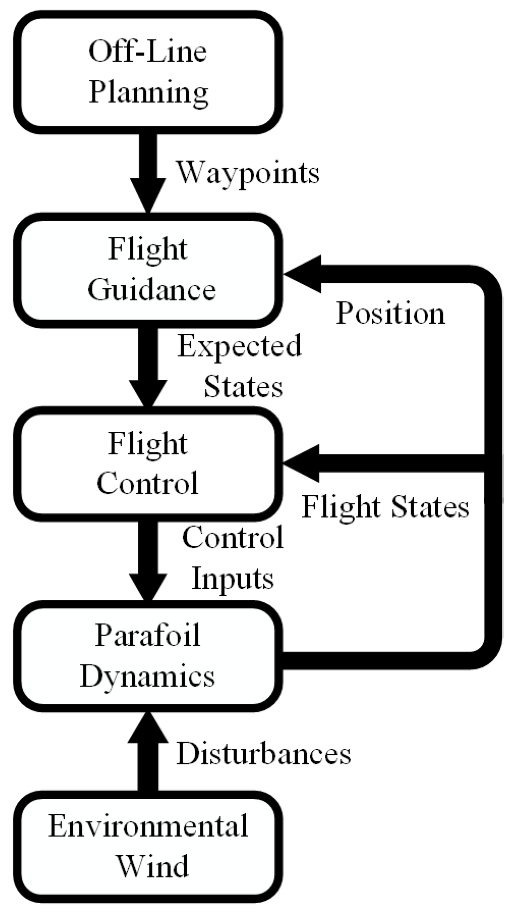
The parafoil typically comprises an upper canopy, a suspended payload, multiple suspension lines, and steering lines. Directional control is effected by pulling down one side of the trailing edge, and a flared landing is achieved by symmetric deflection of both trailing edges. To analyze the parafoil homing method through simulation for different work conditions, a numerical parafoil model with an automatic system is required. Figure 1 depicts the conventional automatic guidance and control system for the parafoil. The process begins with planning an offline reference trajectory from the predetermined airdrop position to the target, which is typically kept fixed throughout the mission. Subsequently, based on the discrete waypoints defining this planned path, the flight guidance and control modules compute the necessary control input for trailing edge deflection to track the trajectory. Ultimately, this system guides the parafoil to a landing in the vicinity of the target.

2.1. Parafoil Dynamics Model

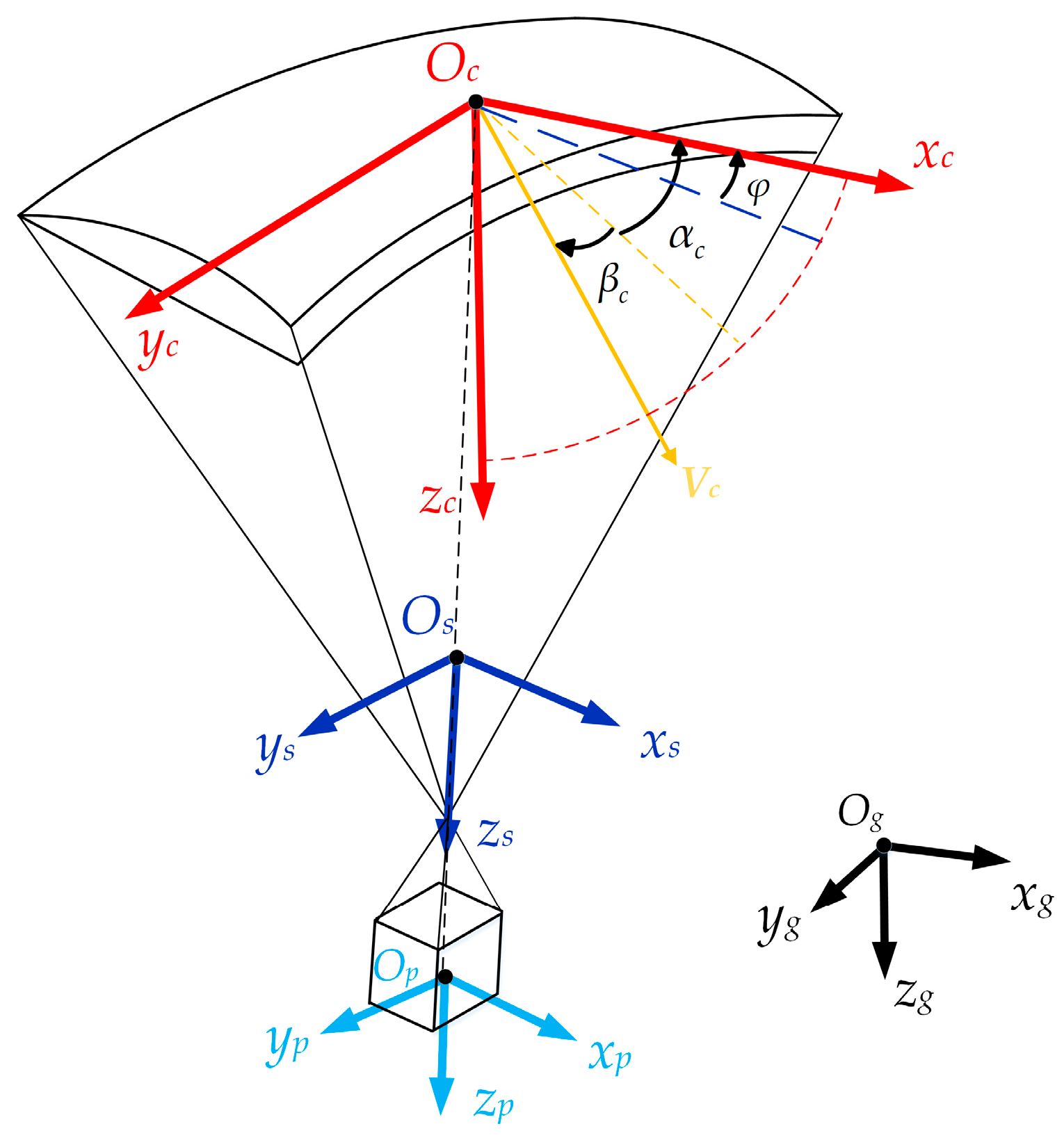
As the foundation of simulation analysis, a six-degree-of-freedom rigid-body model of the parafoil system is established [31,32,33]. The model assumes a fixed geometry between the canopy and the payload, which captures the three translational and three rotational degrees of freedom after the canopy is fully deployed. As illustrated in Figure 2, a north-east-down (NED) ground coordinate system O_gx_gy_gz_g is defined to determine the position of the parafoil. The body-fixed coordinate system O_sx_sy_sz_s is defined with its origin at the system’s center of mass. The x_s-axis is aligned with the longitudinal axis, pointing forward. The z_s-axis points downward along the positive vertical axis, and the y_s-axis completes the right-handed Cartesian system, pointing to the right.

The payload coordinate system denoted as O_px_py_pz_p has its origin at the payload’s center of mass and is aligned with the system frame O_sx_sy_sz_s. The canopy coordinate system O_cx_cy_cz_c is defined by rotating the system frame about the y_s-axis through the incidence angle $\phi$. The origin of this coordinate system is located at the canopy’s center of mass, which coincides with the quarter-chord point. To analyze the aerodynamics of the canopy as the primary lifting surface, the relative airflow angle is used. Specifically, ${\alpha }_c$ is the local angle of attack between the projection of the airspeed vector ${\mathit{V}}_c$ onto the y_c-z_c plane and the x_s-axis. The sideslip angle ${\beta }_c$ is defined as the angle between this airspeed ${\mathit{V}}_c$ projection vector and the airspeed vector.

The rotational and translational dynamics of the parafoil system are governed by a set of differential equations formulated in this body frame. These equations, which account for forces and moments due to aerodynamics, gravity, and apparent mass effects, can be summarized as

$${\dot{\mathit{V}}}_s={(\mathit{m}+{\mathit{m}}_f)}^{-1}({\mathit{F}}_c^a+{\mathit{F}}_c^g+{\mathit{F}}_p^a+{\mathit{F}}_p^g)-\mathbf{\Omega }\times {\mathit{V}}_s$$

(1)

$$\dot{\mathit{H}}={\mathit{M}}_c^a+{\mathit{L}}_c\times {\mathit{F}}_c^a+{\mathit{L}}_p\times {\mathit{F}}_p^a-\mathbf{\Omega }\times \mathit{H}$$

(2)

where ${\mathit{V}}_s={(u,v,w)}^T$ and $\mathbf{\Omega }={(p,q,r)}^T$ are the translational and angular velocity vectors of the system center of mass in the body-fixed frame O_sx_sy_sz_s. m is the generalized mass matrix of the system. ${\mathit{m}}_f$ is the apparent mass matrix accounting for the air enclosed within the canopy. ${\mathit{F}}^a$ and ${\mathit{M}}^a$ are the aerodynamic force and moment vectors. ${\mathit{F}}^g$ is the gravitational force vector. The subscripts c and p denote quantities associated with the canopy and payload, respectively. The displacement vectors of the canopy and payload with respect to the system center of the mass are defined as ${\mathit{L}}_c$ and ${\mathit{L}}_p$. H is the angular momentum vector:

$$\mathit{H}={(\mathit{I}+{\mathit{I}}_f)}^{-1}\mathbf{\Omega }$$

(3)

where I is the inertia matrix, and ${\mathit{I}}_f$ is the inertia matrix induced by the apparent mass.

The differential equation governing attitude angles is given by

$$\dot{\mathbf{\Theta }}=\left[\begin{array}{l}\dot{\varphi }\\ \dot{\theta }\\ \dot{\psi }\end{array}\right]=\left[\begin{array}{ccc}1& s\varphi s\theta /c\theta & c\varphi s\theta /c\theta \\ 0& c\varphi & -s\varphi \\ 0& s\varphi /c\theta & c\varphi /c\theta \end{array}\right]\left[\begin{array}{l}p\\ q\\ r\end{array}\right]$$

(4)

where the vector $\mathbf{\Theta }$ comprises the roll angle $\varphi$, the pitch angle $\theta$, and the yaw angle $\psi$. The yaw angle is defined as the parafoil’s heading relative to true north in the horizontal plane, measured clockwise as positive. The shorthand notations $s(\cdot )$ and $c(\cdot )$ represent $\sin (\cdot )$ and $\cos (\cdot )$, respectively.

The aerodynamic force ${\mathit{F}}_c^a$ and moment ${\mathit{M}}_c^a$ contributed by the canopy are obtained through a sequence of coordinate transformations given by

$${\mathit{F}}_c^a={\displaystyle \frac{1}{2}}\rho V_c^2{S}_c{\mathit{L}}_{cs}^T{\mathit{L}}_{ac}^T\left[\begin{array}{c}-C_D\\ C_Y\\ C_L\end{array}\right]$$

(5)

$${\mathit{M}}_c^a={\displaystyle \frac{1}{2}}\rho V_c^2{S}_c{\mathit{L}}_{cs}^T{\mathit{L}}_{ac}^T\left[\begin{array}{c}-b{C}_l\\ c{C}_m\\ b{C}_n\end{array}\right]$$

(6)

where $\rho$ is the air density. $V_c$ is the local airspeed of the canopy. $S_c$ is the canopy area. $C_D$, $C_Y$, and $C_L$ are the aerodynamic force coefficients. $C_l$, $C_m$, and $C_n$ are the aerodynamic moment coefficients. b is the parafoil span. c is the chord length. ${\mathit{L}}_{cs}$ is the transformation matrix from the system frame to the canopy frame, and ${\mathit{L}}_{ac}$ is the transformation matrix from the canopy frame to the airflow reference frame:

$$L_{cs}=\left[\begin{array}{ccc}c\phi & 0& -s\phi \\ 0& 1& 0\\ s\phi & 0& c\phi \end{array}\right]$$

(7)

$$L_{ac}=\left[\begin{array}{ccc}c{\alpha }_{c}c{\beta }_c& s{\beta }_c& s{\alpha }_{c}c{\beta }_c\\ -c{\alpha }_{c}s{\beta }_c& c{\beta }_c& -s{\alpha }_{c}s{\beta }_c\\ -s{\alpha }_c& 0& c{\alpha }_c\end{array}\right]$$

(8)

The aerodynamic force ${\mathit{F}}_p^a$ contributed by the payload is

$${\mathit{F}}_p^a={\displaystyle \frac{1}{2}}\rho V_p{S}_p{C}_D^p\left[\begin{array}{c}{u}_p\\ v_p\\ w_p\end{array}\right]$$

(9)

where $V_p$ is the local airspeed of the payload; $S_p$ is the maximum cross-sectional area of the payload; $C_D^p$ is the drag coefficient; ${(u_p,v_p,w_p)}^T$ is the velocity vector of the payload.

The aerodynamic coefficients of the parafoil are modeled as functions of inflow angles, angular rates, and control surface deflections. The general form of these coefficients is given by

$$\left\{\begin{array}{l}{C}_D=C_{D0}+C_{D\alpha }{\alpha }_c+C_{D{\alpha }^2}{\alpha }_c^2+C_{D{\delta }_e}{\delta }_e+C_{D{\delta }_a}{\delta }_a\mathrm{sign}({\delta }_a)\\ C_Y=C_{Y\beta }{\beta }_c+C_{Yr}rb/(2V_c)+C_{Y{\delta }_a}{\delta }_a\\ C_L=C_{L0}+C_{L\alpha }{\alpha }_c+C_{L{\alpha }^2}{\alpha }_c^2+C_{L{\delta }_e}{\delta }_e+C_{L{\delta }_a}{\delta }_a\mathrm{sign}({\delta }_a)\\ C_l=C_{l\beta }{\beta }_c+C_{lp}pb/(2V_c)+C_{lr}rb/(2V_c)+C_{l{\delta }_a}{\delta }_a\\ C_m=C_{m0}+C_{m\alpha }{\alpha }_c+C_{mq}qc/(2V_c)+C_{m{\delta }_e}{\delta }_e\\ C_n=C_{n\beta }{\beta }_c+C_{np}pb/(2V_c)+C_{nr}rb/(2V_c)+C_{n{\delta }_a}{\delta }_a\end{array}\right.$$

(10)

where $\mathrm{sign}(\cdot )$ is the sign function; ${\delta }_a$ is the asymmetric trailing-edge deflection used for direction control; ${\delta }_s$ is the symmetric deflection used for height control or speed braking. $C_{D0}$, $C_{L0}$, and $C_{m0}$ denote the drag, lift, and pitch moment baseline aerodynamic coefficients at zero angle of attack, respectively. Their first-order and second-order derivatives with respect to the angle of attack are $\{C_{D\alpha },C_{L\alpha },C_{m\alpha }\}$, and $\left\{C_{D{\alpha }^2},C_{L{\alpha }^2}\right\}$, respectively. The derivatives with respect to the symmetric deflection are $C_{D{\delta }_e}$, $C_{L{\delta }_e}$, and $C_{m{\delta }_e}$. The derivatives with respect to asymmetric deflection are $C_{D{\delta }_a}$, $C_{Y{\delta }_a}$, $C_{L{\delta }_a}$, $C_{l{\delta }_a}$, and $C_{n{\delta }_a}$. The pitch, roll, and yaw damping derivatives are denoted by $C_{mq}$, $\left\{C_{lp},C_{np}\right\}$, and $\left\{C_{lr},C_{nr}\right\}$, respectively. The values of the component stability and control derivatives for each coefficient are obtained from high-fidelity CFD simulations and flight experiments [34].

2.2. Flight Control Module

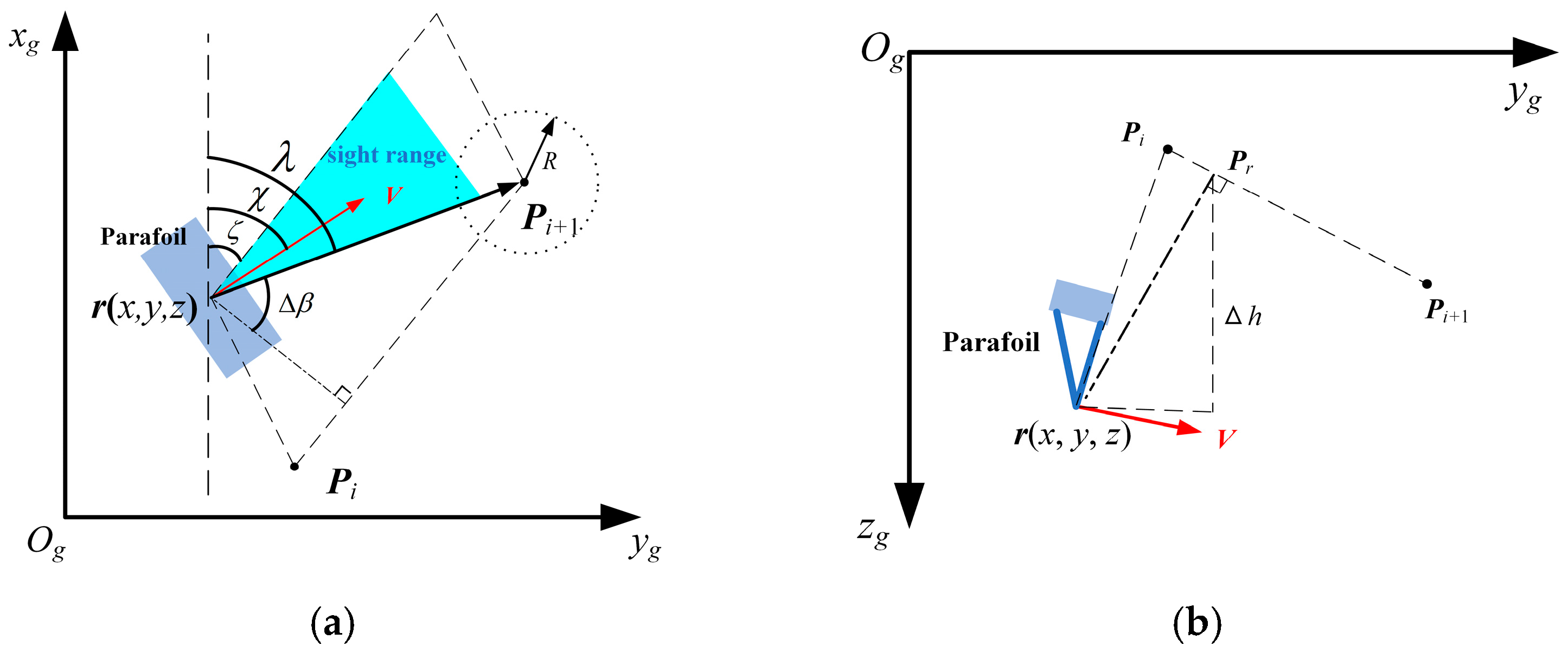
The parafoil is required to follow the planned trajectory until landing, either offline or dynamically replanned online. This reference trajectory is typically defined by a sequence of discrete waypoints $\left\{{\mathit{P}}_0,\cdots {\mathit{P}}_i,\cdots ,{\mathit{P}}_N\right\}$. An autonomous system integrating guidance and control is designed to track this reference. Specifically, a line of sight (LOS) guidance law generates the necessary steering commands for the controller based on the upcoming waypoints [35,36]. As shown in Figure 3a, when the parafoil is navigating between waypoints ${\mathit{P}}_i(x_i,y_i,z_i)$ and ${\mathit{P}}_{i+1}(x_{i+1},y_{i+1},z_{i+1})$ in the geodetic coordinate system, the parallel baseline angle $\zeta$ from ${\mathit{P}}_i$ to ${\mathit{P}}_{i+1}$ is obtained:

$$\zeta =\arctan ((y_{i+1}-y_i)/(x_{i+1}-x_i))$$

(11)

The LOS angle $\lambda$ from the current position r(x, y, z) to the following waypoint ${\mathit{P}}_{i+1}$ is then calculated:

$$\lambda =\arctan ((y_{i+1}-y)/(x_{i+1}-x))$$

(12)

The commanded track angle ${\chi }_d$ is determined by the guidance law within the look-ahead distance:

$${\chi }_d=\zeta +\Delta \chi$$

(13)

where the angle increment $\Delta \chi$ is given by:

$$\Delta \chi =k_s(\lambda -\chi )$$

(14)

where $\chi$ is the actual track angle, and $k_s$ is a guidance gain related to the sight range:

$$k_s={[k_{s1}+k_{s2}\tanh (\left|\right|{\mathit{P}}_{i+1}-\mathit{r}\left|\right|/R)]}^{-1}$$

(15)

where $\tanh (\cdot )$ is the hyperbolic tangent function; $k_{s1}$ and $k_{s2}$ are constant coefficients; R is the waypoint switching radius as illustrated in Figure 3a.

To obtain the height command, the projection position of the current position onto the reference trajectory is determined as illustrated in Figure 3b. The projected point ${\mathit{P}}_r$ is defined as follows:

$${\mathit{P}}_r={\mathit{P}}_i+{\upsilon }_p\stackrel{\_\_\_\_\_\_\_}{{\mathit{P}}_i{\mathit{P}}_{i+1}}$$

(16)

$$\begin{array}{l}{v}_p={\displaystyle \frac{\overline{{\mathit{P}}_i\mathit{r}}\times \overline{{\mathit{P}}_i{\mathit{P}}_{i+1}}}{\left|\right|\overline{{\mathit{P}}_i{\mathit{P}}_{i+1}}|{|}^2}}\\ \hspace{1em}\hspace{0.17em}={\displaystyle \frac{(x-x_i)(x_{i+1}-x_i)+(y-y_i)(y_{i+1}-y_i)+(z-z_i)(z_{i+1}-z_i)}{{(x_{i+1}-x_i)}^2+{(y_{i+1}-y_i)}^2+{(z_{i+1}-z_i)}^2}}\end{array}$$

(17)

The guidance system switches to the next waypoint when the parafoil enters the vicinity of the current target waypoint. Specifically, if either of the conditions is satisfied:

$$\left\{\begin{array}{l}\left|\right|{\mathit{P}}_i-\mathit{r}\left|\right|\le R\\ \Delta \beta =\pi /2-(\lambda -\zeta )\le 0\end{array}\right.$$

(18)

Then the current target waypoint is updated from ${\mathit{P}}_{i+1}$ to ${\mathit{P}}_{i+2}$.

The control system is structured around two primary channels: the direction channel and the height channel. The direction channel generates a differential command for asymmetric control surface deflection to manage track angle, while the height channel generates a collective command for symmetric actuation to adjust height [37]. The LADRC method is employed to track the desired commands according to the following control law [38]:

$$\mathit{U}=\left[\begin{array}{l}{\delta }_s\\ {\delta }_a\end{array}\right]={\mathit{b}}_0^{-1}({\mathit{\omega }}_c^2({\mathit{X}}_d-{\mathit{\sigma }}_1)-2{\mathit{\omega }}_c{\mathit{\sigma }}_2-{\mathit{\sigma }}_3)$$

(19)

where ${\mathit{X}}_d={[{\chi }_d,|z_{P_r}|]}^T$ denotes the state vector, comprising track angle and height; ${\mathit{\omega }}_c$ is a control bandwidth matrix; ${\mathit{b}}_0$ represents the input gain matrix. The estimated state $({\mathit{\sigma }}_1,{\mathit{\sigma }}_2,{\mathit{\sigma }}_3)$ is updated through a linear extended state observer as follows:

$$\left\{\begin{array}{l}{\dot{\mathit{\sigma }}}_1={\mathit{\beta }}_1({\mathit{X}}_d-{\mathit{\sigma }}_1)+{\mathit{\sigma }}_2,\hspace{1em}\hspace{1em} {\mathit{\beta }}_1=3{\mathit{\omega }}_0\\ {\dot{\mathit{\sigma }}}_2={\mathit{\beta }}_2({\mathit{X}}_d-{\mathit{\sigma }}_1)+{\mathit{b}}_0\mathit{U}+{\mathit{\sigma }}_3,{\mathit{\beta }}_2=3{\mathit{\omega }}_0^2\\ {\dot{\mathit{\sigma }}}_3={\mathit{\beta }}_3({\mathit{X}}_d-{\mathit{\sigma }}_1),\hspace{1em}\hspace{1em}\hspace{1em} {\mathit{\beta }}_3={\mathit{\omega }}_0^3\end{array}\right.$$

(20)

where ${\mathit{\omega }}_0$ is the observer gain matrix, typically parameterized by the observer bandwidth.

2.3. Motion Characteristics Analysis

This study employed airdrop experiments to analyze the sensitivity of parafoil dynamics to wind disturbances using an unmanned aerial vehicle (UAV). The parafoil is designed to follow a predetermined flight path, typically featuring a V-type approach. It is released at a calculated distance from the target to ensure sufficient airspace for a safe and controlled descent. A middle key waypoint is set to guide the initial turn of the parafoil and align it with the final approach into the wind. Two airdrop tests were conducted from a height of 150 m under windy conditions.

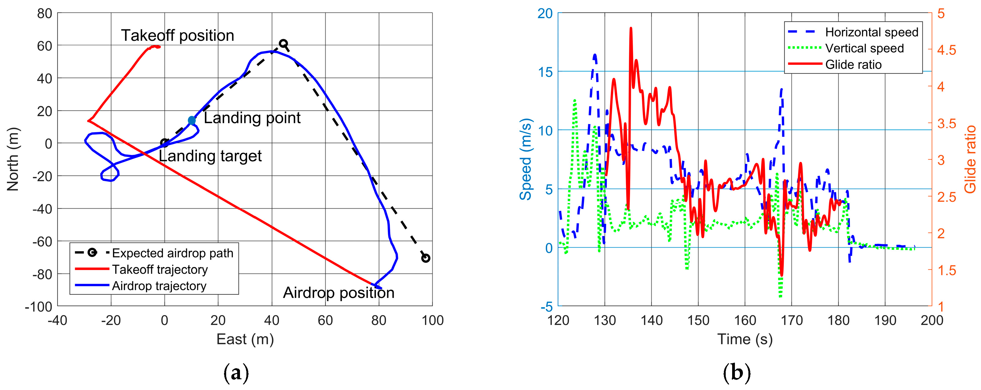
During Test A, there was a south wind recorded at a speed of 1.5 m/s. As shown in Figure 4, during the downwind phase, the parafoil achieved an average horizontal speed of 8.32 m/s and a vertical speed of 2.06 m/s between 132 s and 144 s. After transitioning to the upwind phase for landing, its horizontal speed decreased to 5.29 m/s while maintaining a vertical speed of 2.06 m/s from 150 s to 165 s. Figure 4b illustrates the transient glide ratio of the parafoil under different wind directions, evaluated using a 5 s sliding window to smooth the measurement. During the downwind phase, the parafoil reached a glide ratio of 3.73. Subsequently, when it transitioned to the upwind phase, the glide ratio decreased to 2.62. The distance between the target and the key waypoint was 75 m. The parafoil arrived over the target with excess height and therefore entered an orbiting maneuver to shed the redundant height. Moreover, the turning maneuvers increased the vertical speed and decreased the horizontal speed, thus reducing the glide ratio.

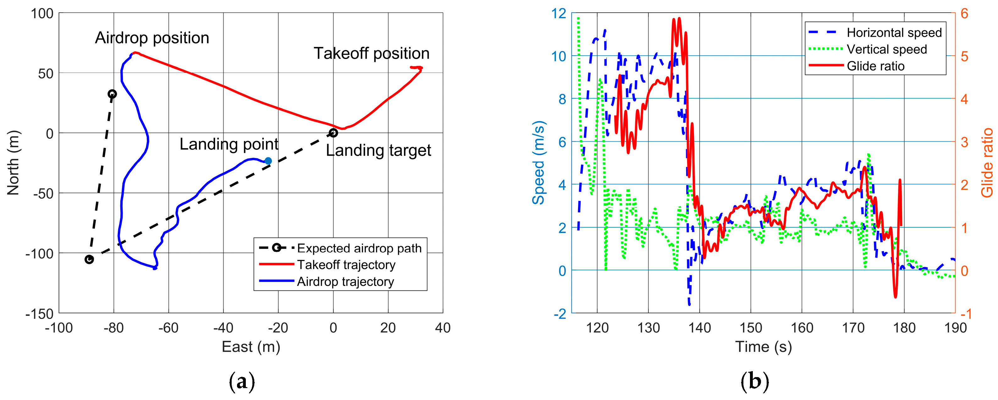
Test B differed from Test A in two primary conditions: the distance from the middle waypoint to the target was increased to 138 m, and the test was conducted in a stronger north wind of 3.3 m/s. As shown in Figure 5a, the enhanced wind resulted in a distinct lateral deviation along the wind direction. Figure 5b further illustrates the wind influence on the flight dynamics. During the downwind phase, the average horizontal speed was 9.02 m/s with a vertical speed of 2.08 m/s from 124 s to 138 s. After transitioning to the upwind phase, the horizontal speed decreased to 3.05 m/s, while the vertical speed remained comparable at 1.99 m/s from 141 s to 179 s. The glide ratio decreased significantly from 4.11 to 1.38 during these two phases because the headwind component altered the effective ground speed, which is the resultant of the airspeed and the wind velocity. The combination of a greater flight distance and the low forward speed during terminal landing contributed to the parafoil touching down short of the target.

According to airdrop test results, the motion of the parafoil can be summarized as the superposition of its basic speed and the wind velocity, as expressed by the following equation [20]:

$$\left\{\begin{array}{l}\dot{x}=V_{hx}={\widehat{V}}_h\cos (\psi )+V_{wh}\cos ({\psi }_w+\pi )\\ \dot{y}=V_{hy}={\widehat{V}}_h\sin (\psi )+V_{wh}\sin ({\psi }_w+\pi )\\ \dot{z}=V_z={\widehat{V}}_z+V_{wz}\\ \dot{\psi }={\overline{\delta }}_a\end{array}\right.$$

(21)

where $({\widehat{V}}_h,{\widehat{V}}_z)$ are the horizontal and vertical airspeed without disturbances, $(V_{wh},V_{wz})$ are the horizontal and vertical components of the wind speed, ${\psi }_w$ is the wind direction angle, defined as the bearing from which the wind originates, measured clockwise from true north, and ${\overline{\delta }}_a$ is the normalized asymmetric control input equal to the yaw angular rate.

The nominal glide performance for a specific parafoil-payload combination is calibrated through preliminary airdrop tests, which provides the reference model for the trajectory planner. An increase in payload mass primarily increases both the horizontal and vertical components of the equilibrium gliding speed, while the glide ratio remains largely unchanged. Therefore, the key parameter requiring adjustment in the kinematic model is the baseline airspeed. For significant mass changes, updating the reference performance parameters in the model is necessary and is a standard operational procedure.

3. Dynamic Replanning Strategy

The unpowered parafoil is highly susceptible to external disturbances, which can cause significant deviations from the planned trajectory. The inherent lack of propulsion means that height tracking errors cannot be rapidly corrected. This problem is exacerbated if the system continues to follow the predefined reference trajectory that is no longer optimal, ultimately leading to a substantial landing error.

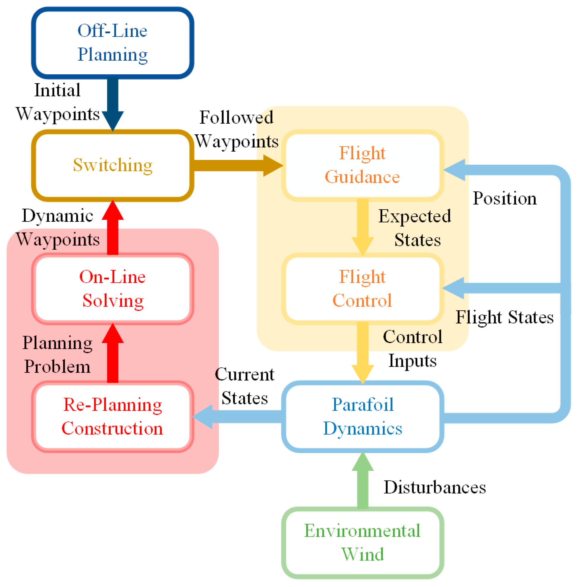
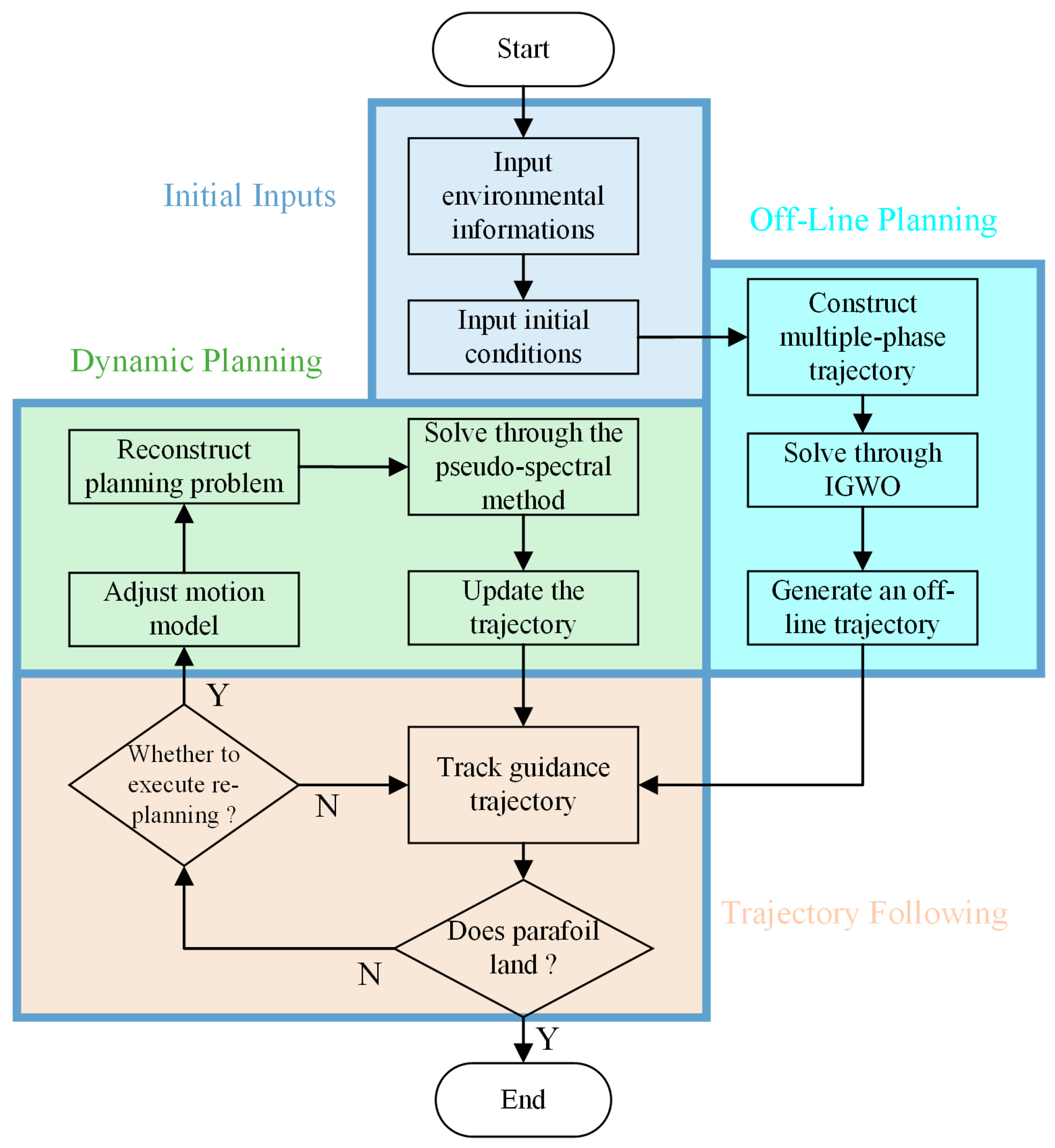
To mitigate these issues, an adaptive online replanning scheme is proposed to enhance the robustness of the parafoil guidance system, whose architecture is depicted in Figure 6. Central to this scheme is the DRP module, which integrates functionalities for trajectory reconstruction and online solution. The workflow operates as follows. The parafoil initially follows a pre-planned offline trajectory. During the flight, the DRP module continuously reconstructs the planning problem based on current states and then solves it in real-time to generate an updated trajectory. This new trajectory is subsequently executed via a trajectory-switching module. The strategy allows for multiple iterative adjustments throughout the remaining flight to ensure continuous and accurate target approach.

There is a cooperation effect to mitigate external disturbances: (1) the DRP module compensates for accumulated trajectory deviations through successive online updates operating on a slow-time scale, and (2) the flight control system tracks the updated trajectory against transient disturbances on a fast-time scale.

3.1. Layered Planning

3.1.1. Multi-Phase Trajectory Design

During flight, the parafoil is designed to follow a precomputed trajectory under the command of a feedback guidance and control system. To compensate for deviations and mitigate error accumulation, the replanning strategy is implemented. However, trajectories generated by the APSM generally occupy a larger airspace to dissipate excess height, which can leave insufficient space for precise terminal adjustment. The proposed guidance strategy initiates with a multi-phase trajectory computed using the IGWO algorithm. The primary objective of this strategy is to guide the parafoil to the target efficiently while ensuring adequate height margin for the execution of DRP.

Figure 6. Work frame of the automatic following system with DRP.

Figure 6. Work frame of the automatic following system with DRP.

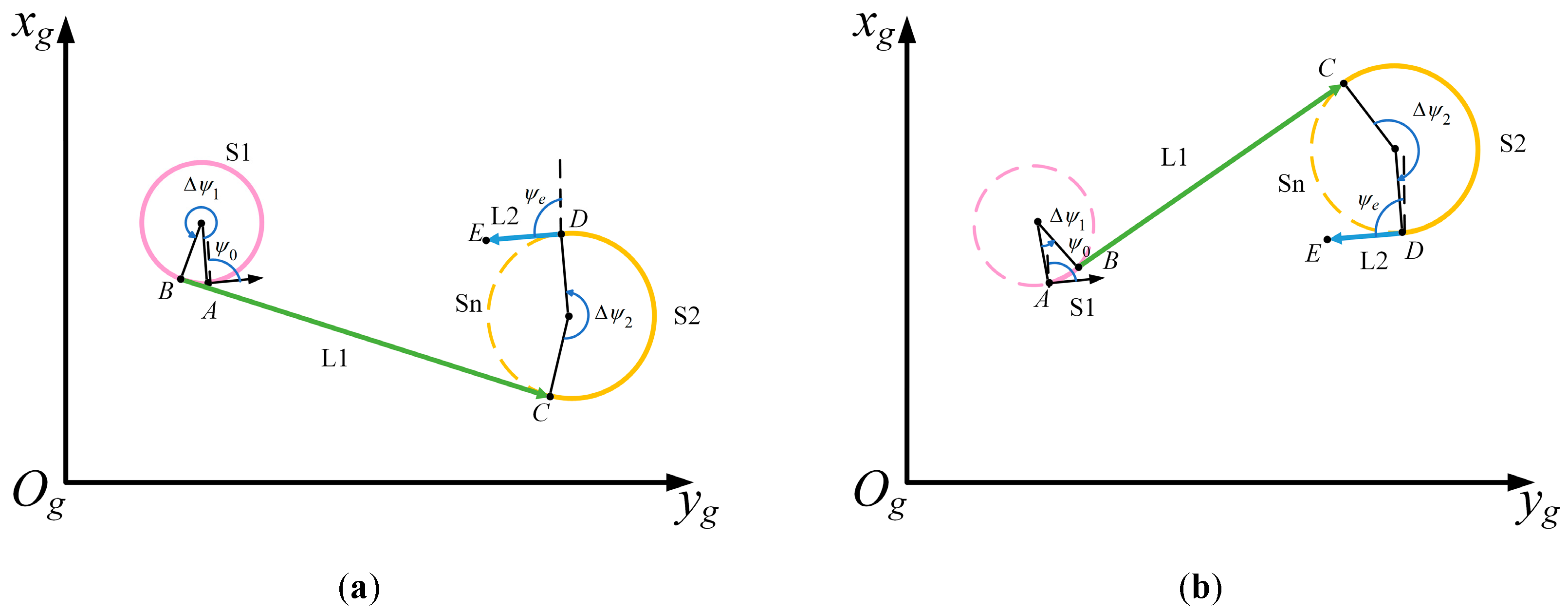
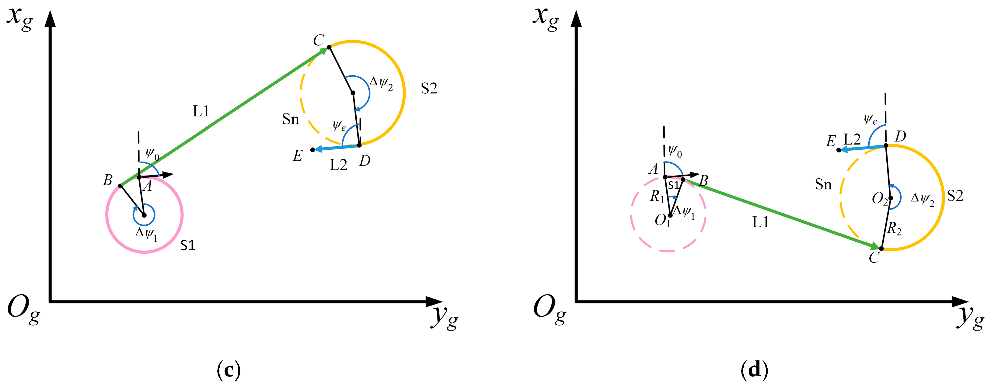
The homing trajectory is divided into four sequential phases, as illustrated in Figure 7: (AB) direction adjustment, (BC) straight glide, (CD) height reduction via circling, and (DE) flared landing. The Dubins curve is employed to generate the segmented trajectory [8]. Let n₁ $\in$ {−1, 1} define the turning direction of the initial adjustment phase (AB), viewed from above, where n₁ = −1 denotes a counterclockwise (CCW) turn. Similarly, the turning direction for the height reduction phase (CD) is defined by n₂ $\in$ {−1, 1}. For computational simplicity and to ensure a coordinated maneuver, the turning direction of the height reduction phase is set to be opposite to that of the initial adjustment phase, i.e., n₁ = −n₂. Given a fixed initial yaw angle ${\psi }_0$ and a required landing direction ${\psi }_e$, there exist four distinct geometric configurations (G₁, G₂, G₃, G₄) for the composite Dubins path. These configurations correspond to the feasible combinations of the turning directions that satisfy the boundary conditions.

Given the initial position ${\mathit{r}}_0$ and the target position ${\mathit{r}}_e$, the center coordinates of the Dubins circles S1 and S2, denoted as ${\mathit{r}}_{O_1}$ and ${\mathit{r}}_{O_2}$, can be calculated. The calculation accounts for the geometry of the final approach and is given by the following equations:

$$\left[\begin{array}{l}{r}_{O_1.x}\\ r_{O_1.y}\end{array}\right]=\left[\begin{array}{l}{r}_{0.x}+R_1\cos ({\psi }_0+n_1\pi /2)\\ r_{0.y}+R_1\sin ({\psi }_0+n_1\pi /2)\end{array}\right]$$

(22)

$$\left[\begin{array}{l}{r}_{O_2.x}\\ r_{O_2.y}\end{array}\right]=\left[\begin{array}{l}{r}_{e.x}+l_s\cos ({\psi }_e)+R_2\cos ({\psi }_e+n_2\pi /2)\\ r_{e.y}+l_s\sin ({\psi }_e)+R_2\sin ({\psi }_e+n_2\pi /2)\end{array}\right]$$

(23)

where $l_s$ is the flare initiation distance; ${\psi }_e$ is the final heading angle for landing; $R_1$ and $R_2$ are the radii of circles S1 and S2, respectively.

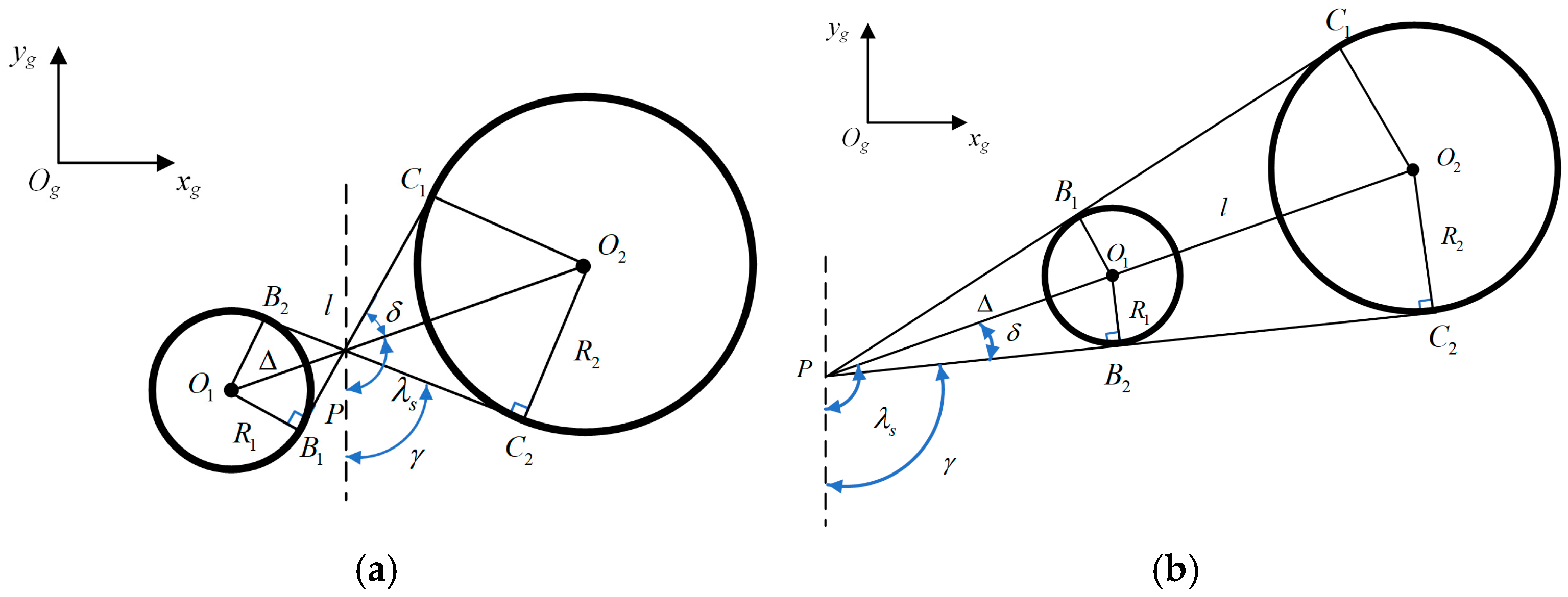
As shown in Figure 8, the locations of the feature nodes change with the trajectory profile configuration. The coordinates of the intersection point P, defined by two tangent lines $\stackrel{\_\_\_\_\_}{{\mathit{B}}_1{\mathit{C}}_1}$ and $\stackrel{\_\_\_\_\_}{{\mathit{B}}_2{\mathit{C}}_2}$, are given by

$${\mathit{r}}_P={\mathit{r}}_{O_1}\pm \Delta ({\mathit{r}}_{O_2}-{\mathit{r}}_{O_1})/l$$

(24)

where l is the distance between the centers of circles S1 and S2. The second term in Equation (24) represents the horizontal offset of point P, and its sign (positive or negative) corresponds to the two scenarios depicted in Figure 8. The distance $\Delta$ from point P to O₁ is expressed as follows:

$$\Delta =l{R}_1/(R_2\pm R_1)$$

(25)

Thus, the coordinates of key geometric nodes are obtained as follows:

$$\left[\begin{array}{l}{r}_{B.x}\\ r_{B.y}\end{array}\right]=\left[\begin{array}{l}{r}_{P.x}\\ r_{P.y}\end{array}\right]+\mathrm{sign}(r_{O_1.x}-r_{O_2.x})\sqrt{{\Delta }^2-R_1^2}\left[\begin{array}{l}\cos (\gamma )\\ \sin (\gamma )\end{array}\right]$$

(26)

$$\left[\begin{array}{l}{r}_{C.x}\\ r_{C.y}\end{array}\right]=\left[\begin{array}{l}{r}_{P.x}\\ r_{P.y}\end{array}\right]+\mathrm{sign}(r_{O_1.x}-r_{O_2.x})\sqrt{{\Delta }^2+R_1^2}\left[\begin{array}{l}\cos (\gamma )\\ \sin (\gamma )\end{array}\right]$$

(27)

where $\gamma$ is the slope angle of the tangent line:

$$\gamma ={\lambda }_s\pm \delta =\arctan ((r_{O_2.y}-r_{O_1.y})/(r_{O_2.x}-r_{O_1.x}))\pm \arctan (R_1/\Delta )$$

(28)

where ${\lambda }_s$ is the slope angle of the line connecting the centers of the two circles, and $\delta$ is the half-angle between the bitangent lines. Specifically, the positive and negative signs of the second term designate the upper and lower bitangent pairs, $\stackrel{\_\_\_\_\_}{{\mathit{B}}_1{\mathit{C}}_1}$ and $\stackrel{\_\_\_\_\_}{{\mathit{B}}_2{\mathit{C}}_2}$, respectively.

The length of each trajectory phase can be estimated after the feature nodes are determined, as shown in the following equation:

$$\left\{\begin{array}{l}{L}_1=R_1\Delta {\psi }_1\\ L_2=\left|\right|{\mathit{r}}_C-{\mathit{r}}_B\left|\right|\\ L_3=R_2(\Delta {\psi }_2+2\pi N_{cir})\\ L_4=l_s\end{array}\right.$$

(29)

where $N_{cir}$ is the number of circling maneuvers counted from the highest point above the flared landing beginning point.

The total height $\tilde{H}$ of the planned trajectory must satisfy the actual airdrop height constraint $H_{total}$. Therefore, the trajectory planning problem is transformed into an optimization problem for the feature parameters, subject to the following constraints:

$$\min J=|\tilde{H}(R_1,R_2,N_{cir})-H_{total}|$$

(30)

subject to

$$\left\{\begin{array}{l}{R}_1,R_2\ge R_{\min }\\ \mathrm{int}(N_{cir})-N_{cir}=0\end{array}\right.$$

(31)

where $R_{\min }$ is the minimum turning radius, and int(·) denotes the ceiling function.

To account for the vertical variation in wind speed and direction, each trajectory segment is discretized into several consecutive elements. The total descent height is then estimated as follows:

$$\tilde{H}={\displaystyle \sum _{i=1}^4{\displaystyle \sum _{j=1}^{N_i}\frac{L_i}{N_i{k}_{ij}}}}$$

(32)

where $N_i$ is the number of elements within the segment, and $k_{ij}$ is the glide ratio of the i-th element.

The wind influences the glide ratio of the parafoil because the wind alters the ground speed, which is the vector sum of its airspeed and the wind velocity. Consequently, the transient glide ratio at a flight level can be expressed as a function of the wind inflow angle:

$$k={\displaystyle \frac{\sqrt{{({\widehat{V}}_h\cos (\psi )+V_{wh}\cos ({\psi }_w+\pi ))}^2+{({\widehat{V}}_h\sin (\psi )+V_{wh}\sin ({\psi }_w+\pi ))}^2}}{{\widehat{V}}_z+V_{wz}}}$$

(33)

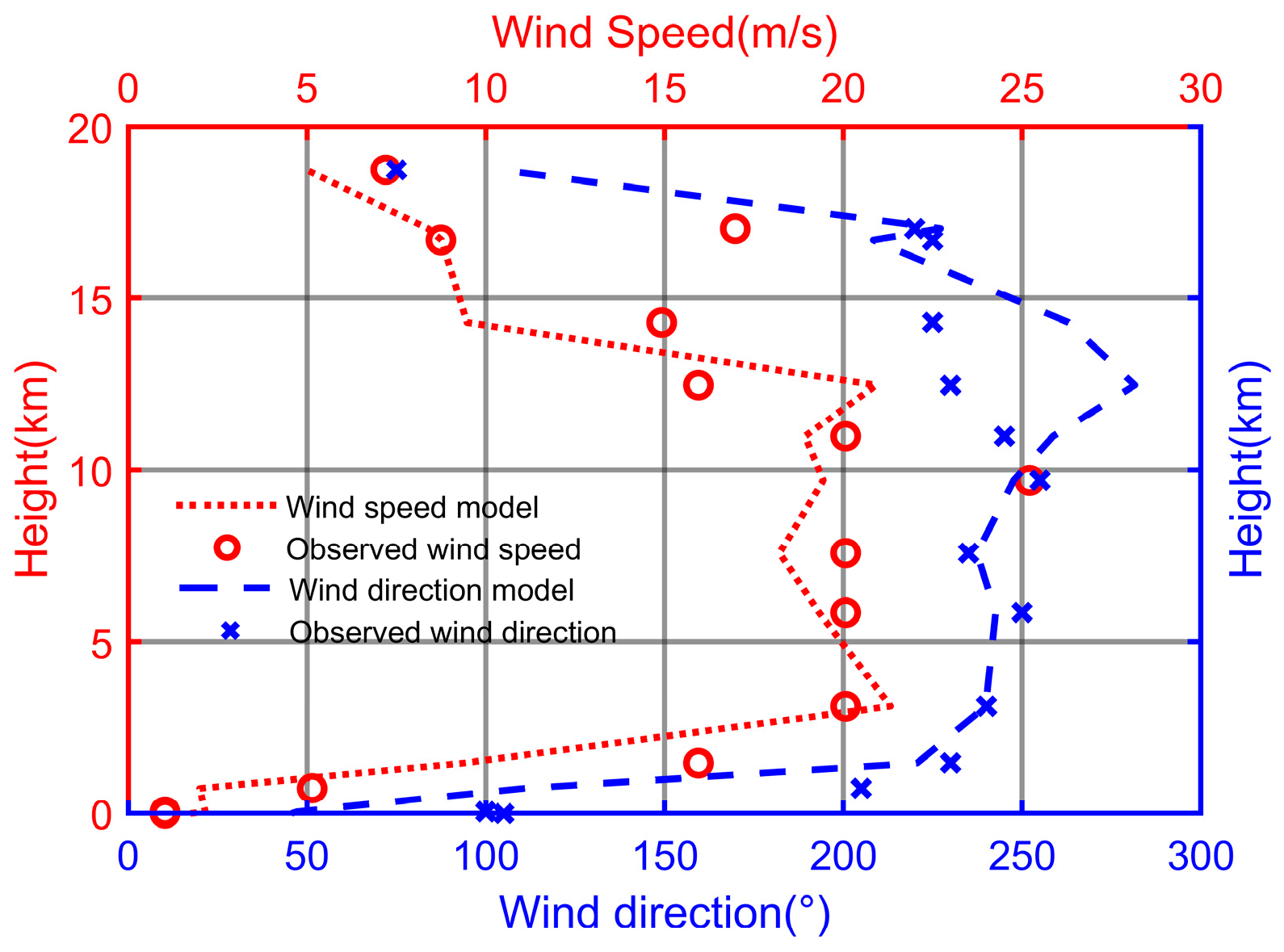
Based on a numerical weather prediction model, the environmental wind field is constructed by assimilating observed atmospheric data and terrain information [39]. This model primarily characterizes the mean wind profile, capturing the variations in wind speed and direction with height. As shown in Figure 9, the resulting height profile of the wind field for a specific area is displayed, illustrating the characteristic wind present during the test period. A comparison between the modeled wind profile and actual sounding observations indicates a high level of consistency. Given that the mean vertical wind in the operational flight envelope is generally much smaller than the horizontal component, its value is set to zero or to a minimal constant.

3.1.2. Key Parameter Solving

The optimization expression in Equation (30) poses significant challenges for numerical optimization due to the presence of the integer variable $N_{cir}$, which represents the circling number. Traditional gradient-based methods are unsuitable for such problems because they are difficult to handle discrete variables efficiently. To address this, the gray wolf optimizer (GWO) is employed. This algorithm mimics the social hierarchy and collaborative hunting behavior of gray wolves to optimize the key parameter vector X = ($R_1$, $R_2$, $N_{cir}$)^T$\in$ ${\mathit{R}}^3$ of the segment trajectory. In the GWO framework, the entire population forms a set $\mathit{P}=\{{\mathit{X}}_1,\cdots ,{\mathit{X}}_i,\cdots ,{\mathit{X}}_{W_n}\}$, and each wolf’s position in the search space encodes a candidate solution ${\mathit{X}}_i$. The fittest three solutions are designated as the alpha ($\alpha$), beta ($\beta$), and delta ($\delta$) wolves, which guide the search. The remaining solutions are referred to as omega ($\omega$) wolves and follow the leading wolves.

Each individual wolf in the pack moves toward the leading wolves to encircle the prey, generating a new candidate position according to the following update rule at the iteration step t:

$${\widehat{\mathit{X}}}_i(t+1)=f_{i\alpha }{\mathit{X}}_{i\alpha }(t)+f_{i\beta }{\mathit{X}}_{i\beta }(t)+f_{i\delta }{\mathit{X}}_{i\delta }(t)$$

(34)

where ${\mathit{X}}_{ik}(k=\alpha ,\beta ,\delta )$ denotes the guided position generated by the leading wolf for the i-th wolf in the pack. $f_{ik}$ is the weight coefficient derived from the optimal fitness value of the leading wolf. The guided position is calculated as follows:

$${\mathit{X}}_{ik}={\mathit{X}}_k-\mathit{A}\times \mathit{D}$$

(35)

$$\mathit{D}=|\mathit{C}\times {\mathit{X}}_k-{\mathit{X}}_i|$$

(36)

The coefficient vectors A and C are calculated as follows:

$$\mathit{A}=2\mathit{a}\times {\mathit{r}}_1-\mathit{a}(t)$$

(37)

$$\mathit{C}=2{\mathit{r}}_2$$

(38)

where ${\mathit{r}}_1$ and ${\mathit{r}}_2$ are random vectors with elements uniformly distributed in the range [0, 1]. The components of the vector a decrease linearly from 2 to 0 over the course of the iterations, thereby shifting the search behavior of the wolf pack from global exploration to local exploitation.

To balance exploration and exploitation while maintaining population diversity, a cooperative learning mechanism is implemented among neighboring individuals [40]. The neighborhood around the current solution ${\mathit{X}}_i$ is defined as follows:

$${\mathit{N}}_i(t)=\left\{{\mathit{X}}_j(t)|{\mathit{D}}_i\left({\mathit{X}}_i(t),{\mathit{X}}_j(t)\right)\le {\mathit{R}}_i(t),{\mathit{X}}_j(t)\in \mathit{P}\right\}$$

(39)

where the neighborhood radius is expressed as:

$${\mathit{R}}_i(t)=|{\mathit{X}}_i(t)-{\widehat{\mathit{X}}}_i(t+1)|$$

(40)

The new candidate position ${\widehat{\mathit{X}}}_{i\text{-}D}(t+1)$ is generated by randomly selecting an individual ${\mathit{X}}_n(t)$ from the neighborhood ${\mathit{N}}_i(t)$ and another individual ${\mathit{X}}_r(t)$ from the entire population P. The element in its d-th (d = 1, 2, 3) dimension is calculated by:

$${\widehat{\mathit{X}}}_{i\text{-}D,d}(t+1)={\mathit{X}}_{i,d}(t)+{\mathit{r}}_{3,d}({\mathit{X}}_{n,d}(t)-{\mathit{X}}_{r,d}(t))$$

(41)

where ${\mathit{r}}_3$ is a random vector with elements uniformly distributed in the range [0, 1].

The two candidate positions, ${\widehat{\mathit{X}}}_i(t+1)$ generated by the standard GWO strategy and ${\widehat{\mathit{X}}}_{i\text{-}D}(t+1)$ generated by the dimension-learning strategy, are evaluated using the fitness function. The candidate with the best fitness value is selected to update the position for the next iteration.

3.2. Trajectory Updating

3.2.1. Optimization Reformulation

As shown in Figure 10, after the parafoil approaches the target by following the initial offline trajectory, the APSM is used to compute the trajectory that is compliant with the parafoil’s glide constraints. The underlying optimal control problem incorporating the motion dynamics is formulated as follows [20]:

$$\min J=w_1\left|\right|\mathit{r}(t_f)-{\widehat{\mathit{r}}}_{t_f}\left|\right|+w_2{\displaystyle {\int }_{t_0}^{t_f}\left|\right|\mathit{U}|{|}^{2}dt}$$

(42)

subject to

$$\left\{\begin{array}{l}\dot{\mathit{X}}=\mathit{f}(\mathit{X},\mathit{U},t)\\ {\mathit{X}}_{\max }\ge \mathit{X}\ge {\mathit{X}}_{\min }\\ {\mathit{U}}_{\max }\ge \mathit{U}\ge {\mathit{U}}_{\min }\\ \mathit{X}(t_0)={\mathit{X}}_{t_0}\\ \mathit{X}(t_f)={\mathit{X}}_{t_f}\end{array}\right.$$

(43)

where $t_0$ and $t_f$ are the initial and final time of the planning horizon, respectively. The position vector $\mathit{r}(t)$ is a function of time. ${\widehat{\mathit{r}}}_{t_f}$ is the expected landing position. $w_1$ and $w_2$ are the weights for the landing precision and control effort, respectively. $\dot{\mathit{X}}=\mathit{f}(\mathit{X},\mathit{U},t)$ denote the system equation of motion in Equation (21). The system state and control input fall within the available ranges of $[{\mathit{X}}_{\min },{\mathit{X}}_{\max }]$ and $[{\mathit{U}}_{\min },{\mathit{U}}_{\max }]$, respectively. $\mathit{X}(t_0)={\mathit{X}}_{t_0}$ and $\mathit{X}(t_f)={\mathit{X}}_{t_f}$ indicate the initial and final state conditions.

In each replanning cycle, the optimization problem is reconstructed using updated parameters, including wind field information, the current flight position, and heading. According to the zero-sideslip angle condition, it is assumed that the track direction aligns with the longitudinal axis of the parafoil at the end of the planned trajectory. The initial heading constraint and the terminal constraint requiring the parafoil to face into the wind are given by

$${\psi }_{t_0}={\psi }_{cur}$$

(44)

$${\psi }_{t_f}={\psi }_{we}+\pi$$

(45)

where ${\psi }_{cur}$ is the current yaw angle of the parafoil, and ${\psi }_{we}$ is the surface wind direction.

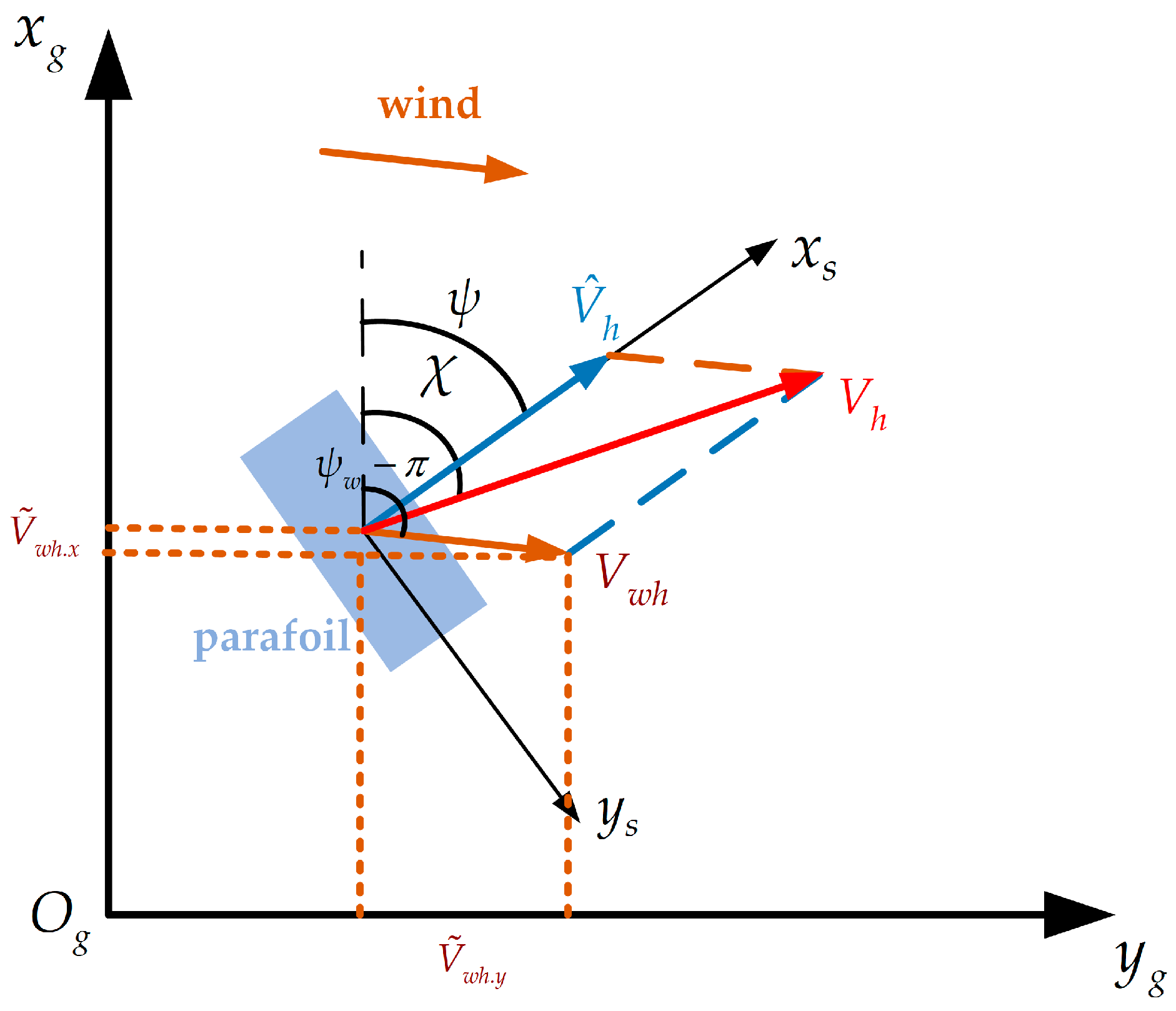
Figure 11 schematically illustrates the decomposition of the ground velocity into its airspeed and the ambient wind velocity in the horizontal plane. To estimate the time-varying wind field, a sliding window approach is applied. The algorithm inputs include the measured ground speed, yaw angle, and sideslip angle. The wind speed and direction at each time step are approximated as follows:

$$V_{wh}=\sqrt{{\tilde{V}}_{wh.x}^2+{\tilde{V}}_{wh.y}^2}$$

(46)

$${\psi }_w=\arctan ({\tilde{V}}_{wh.y}/{\tilde{V}}_{wh.x})+\pi$$

(47)

where the estimated wind components are calculated as follows:

$${\tilde{V}}_{wh.x}=V_h\cos (\chi )-{\widehat{V}}_h\cos (\psi )$$

(48)

$${\tilde{V}}_{wh.y}=V_h\sin (\chi )-{\widehat{V}}_h\sin (\psi )$$

(49)

where $V_h$ and ${\widehat{V}}_h$ are the measured ground velocity and baseline airspeed, respectively.

3.2.2. Discretization and Solving

The solution to the continuous-time optimization requires a discrete-time formulation. Before discretization, time normalization is carried out on the time variable as follows:

$$\tau ={\displaystyle \frac{2}{t_f-t_0}}(t-{\displaystyle \frac{t_f+t_0}{2}})$$

(50)

The variables of the system and input on the scaled time are given through the Lagrange interpolation:

$$\mathit{X}(\tau )={\displaystyle \sum _{i=0}^N{L}_i(\tau )\mathit{X}({\tau }_i)}$$

(51)

$$\mathit{U}(\tau )={\displaystyle \sum _{i=1}^N{\tilde{L}}_i(\tau )\mathit{U}({\tau }_i)}$$

(52)

where $L_i(\tau )$ and ${\tilde{L}}_i(\tau )(i\ne 0)$ represent the Nth-order and the (N − 1)th-order Lagrange polynomials, respectively:

$$L_i(\tau )={\displaystyle \prod _{j=0,j\ne i}^N\frac{\tau -{\tau }_j}{{\tau }_i-{\tau }_j}}$$

(53)

$${\tilde{L}}_i(\tau )={\displaystyle \prod _{j=1,j\ne i}^N\frac{\tau -{\tau }_j}{{\tau }_i-{\tau }_j}}$$

(54)

The variable ${\tau }_k(k=1,\dots ,N)$ denotes a Legendre-Gauss collocation point, defined as a root of the Nth-order Legendre polynomial. Further, the initial time point ${\tau }_0=-1$ is included in the discrete time set to enforce the initial condition $\mathit{X}(t_0)={\mathit{X}}_{t_0}$. The state at the final point ${\tau }_{N+1}=1$ is then approximated using the Gauss quadrature rule as follows:

$$\mathit{X}({\tau }_f)=\mathit{X}({\tau }_0)+{\displaystyle \frac{t_f-t_0}{2}}{\displaystyle \sum _{k=1}^N{\omega }_k\mathit{f}(\mathit{X}({\tau }_k),\mathit{U}({\tau }_k),{\tau }_k)}$$

(55)

where ${\omega }_k$ is the Gauss integration weight.

Finally, the discrete NLP derived from the original continuous optimal control problem is formulated as follows:

$$\min J=w_1||\mathit{r}({\tau }_f)-{\widehat{\mathit{r}}}_{{\tau }_f}||+w_2{\displaystyle \frac{t_f-t_0}{2}}{\displaystyle \sum _{k=0}^N\left|\right|\mathit{U}|{|}^2}$$

(56)

subject to

$$\left\{\begin{array}{l}{\displaystyle \sum _{i=0}^N{\dot{L}}_i({\tau }_k){\mathit{X}}_i}={\displaystyle \frac{t_f-t_0}{2}}\mathit{f}(\mathit{X}({\tau }_k),\mathit{U}({\tau }_k),{\tau }_k)\\ {\mathit{X}}_{\max }\ge \mathit{X}({\tau }_k)\ge {\mathit{X}}_{\min }\\ {\mathit{U}}_{\max }\ge \mathit{U}({\tau }_k)\ge {\mathit{U}}_{\min }\\ \mathit{X}({\tau }_0)={\mathit{X}}_{{\tau }_0}\\ \mathit{X}({\tau }_k)=\mathit{X}({\tau }_0)+{\displaystyle \frac{t_f-t_0}{2}}{\displaystyle \sum _{k=1}^N{\omega }_k\mathit{f}(\mathit{X}({\tau }_k),\mathit{U}({\tau }_k),{\tau }_k)}\end{array}\right.$$

(57)

The above discrete optimization problem is solved numerically using a sequential quadratic programming (SQP) method. The SQP algorithm iteratively solves a series of quadratic programming subproblems that approximate the original NLP locally around the current iterate. The solution yields a sequence of discrete states and control inputs at the collocation points. For each subsequent replanning cycle, this solving process is repeated, starting from the latest estimated system state, thereby enabling real-time correction and refinement of the guidance trajectory.

4. Simulation and Experiment

4.1. DRP Verification

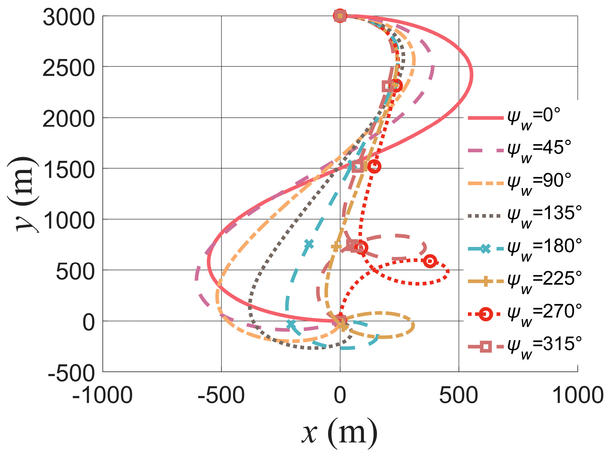
As shown in Figure 12, the parafoil simulation starts from an initial position of (0, 3000, −2000) m with zero initial heading, targeting the origin of the ground coordinate system. multiple trajectories are generated from a common starting point to the origin based on the APSM, each designed for a different wind direction. These trajectories account for the dominant steady wind component and ensure the parafoil can execute a flared landing into the wind, with the wind direction ${\psi }_w$ ranging from 0 to 315 degrees.

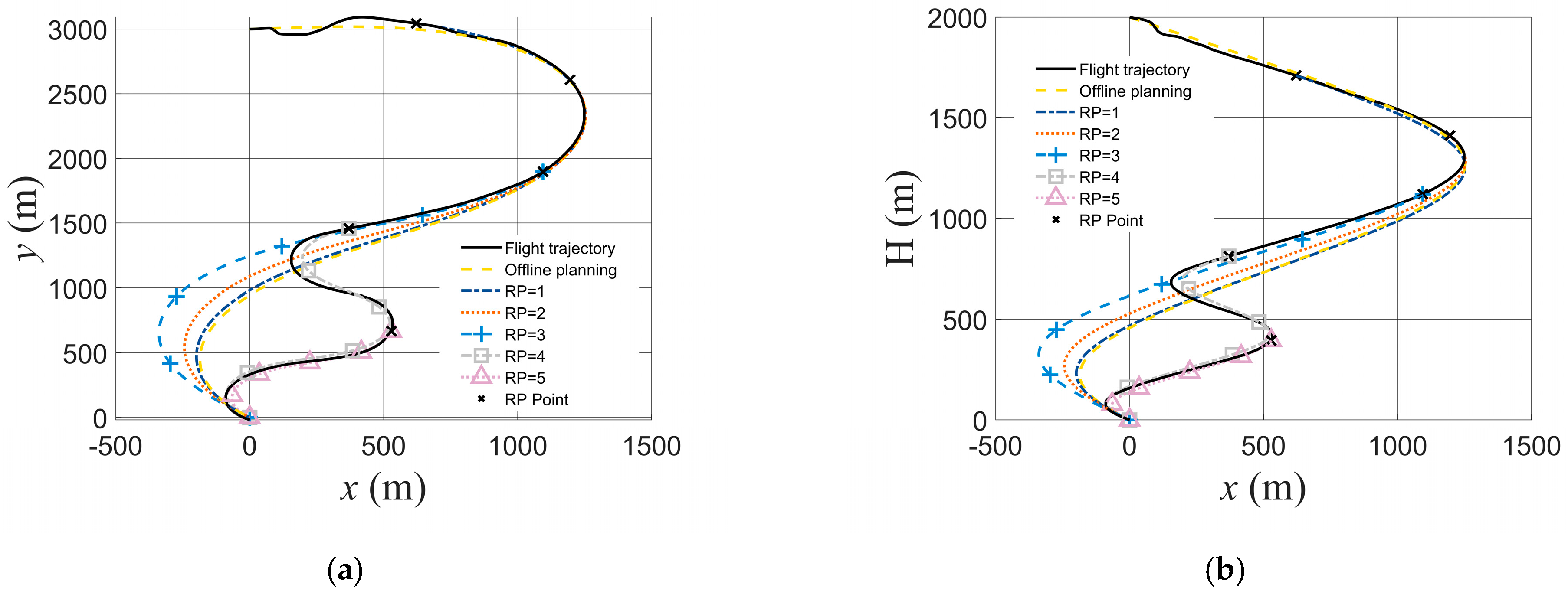
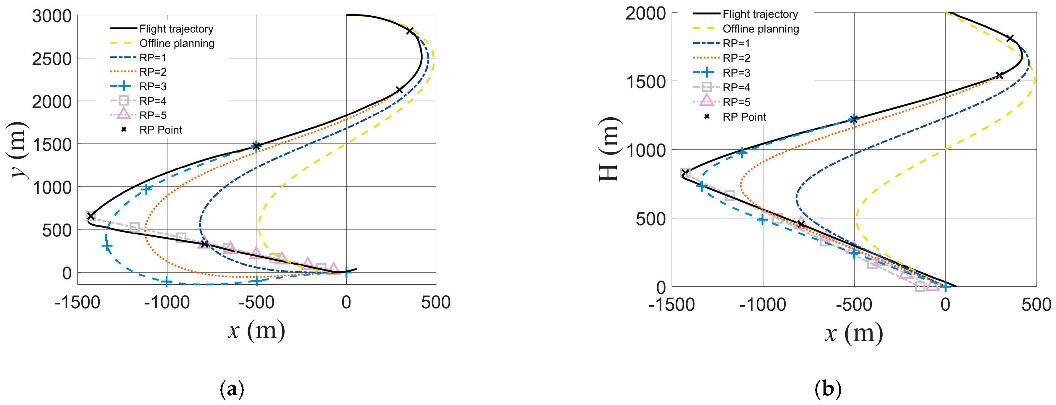
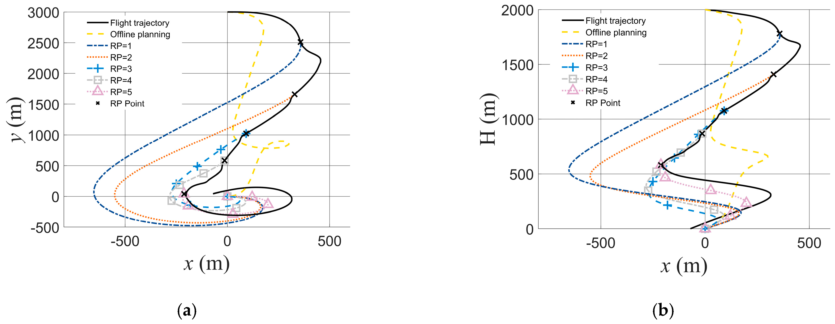
The parafoil is designed to follow a predefined trajectory. Upon reaching a specified height, the DRP process is initiated to update the reference trajectory. Flight simulations are conducted with a limit of up to five RP cycles to validate the process. The performance of the dynamic planning strategy is evaluated under varying wind disturbances. As shown in Figure 13, the parafoil achieves accurate trajectory tracking with a minimal landing error of (0.8, −19.3) m under a mild 1 m/s wind. When wind intensity increases, the replanning mechanism becomes more active. As shown in Figure 14, the first three updates extend the trajectory horizontally to exploit glide performance, but a lateral wind-induced deviation of about 137 m at the fourth point necessitates a compensatory shortening of the remaining path, resulting in a final error of (60.1, 42.6) m. In Figure 15, the 5 m/s wind leads to a significant initial deviation after release. The proposed method mitigates this error from over 200 m to 80 m through successive replanning, which involves dynamic adjustments in both distance and height to cope with disturbances, culminating in a landing error of (−70.4, 42.0) m. These results underscore the strategy’s robustness in managing uncertainties across different wind conditions.

It is noted that since the parafoil must land into the wind, a weaker headwind typically requires a longer descent glide distance to fully dissipate the available height. As shown in Figure 13, under a light wind condition (1 m/s), the planner generates a relatively longer gliding trajectory to ensure the redundant height is completely expended before reaching the target. Conversely, a strong wind (5 m/s) overall reduces the glide ratio. Therefore, as shown in Figure 15, the corresponding horizontal gliding distance is correspondingly shorter.

The effective ground glide ratio decreases when flying into a headwind, a principle clearly illustrated in the resulting trajectories under different wind conditions. In Figure 15, the parafoil encounters a predominant headwind throughout most of the descent between approximately 1700 m to 600 m in height as it approaches the target. This causes a significant degradation in ground glide performance, thereby reducing the total glide distance and resulting in a more direct trajectory. In contrast, Figure 14 presents a different scenario. Between approximately 1700 m and 800 m in height, the parafoil’s heading relative to the wind shifts, placing it in a tailwind condition. This yields a higher effective glide ratio, necessitating a longer flight path to dissipate the height, thereby accounting for the extended lateral range observed.

4.2. Combined Homing Strategy

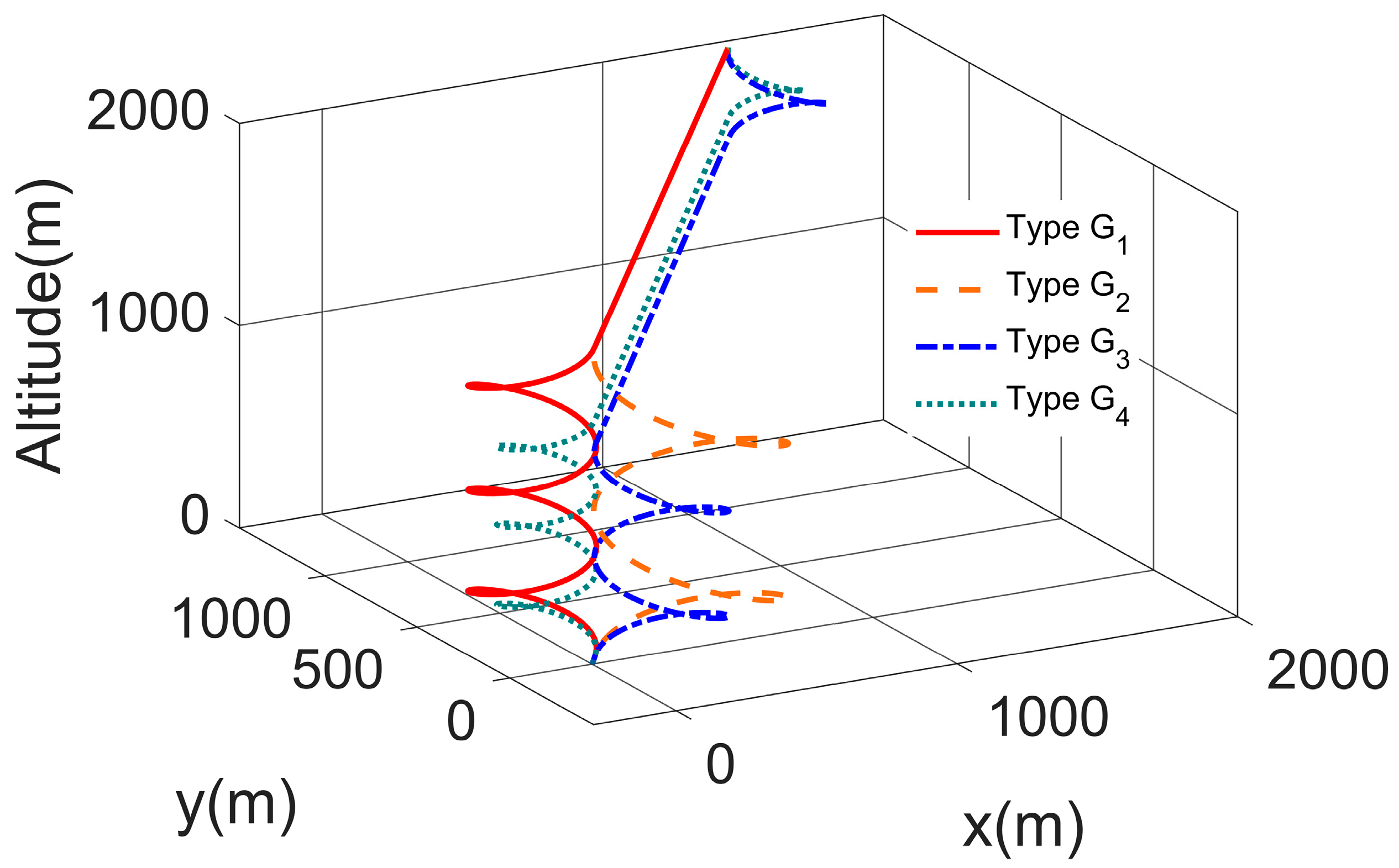
The initial state of the parafoil system is set at the position (1414.2, 1414.2, −2000) m with a yaw angle of 228.14 degrees. The landing target is set at the origin of the ground coordinate system. The landing direction is determined to be 225.94 degrees, which is consistent with wind direction to achieve an into-wind touchdown. The segmented trajectory is computed using the IGWO method, configured with a population of 30 search agents and a maximum of 500 iterations. Figure 16 displays the resulting trajectories for different geometric configurations.

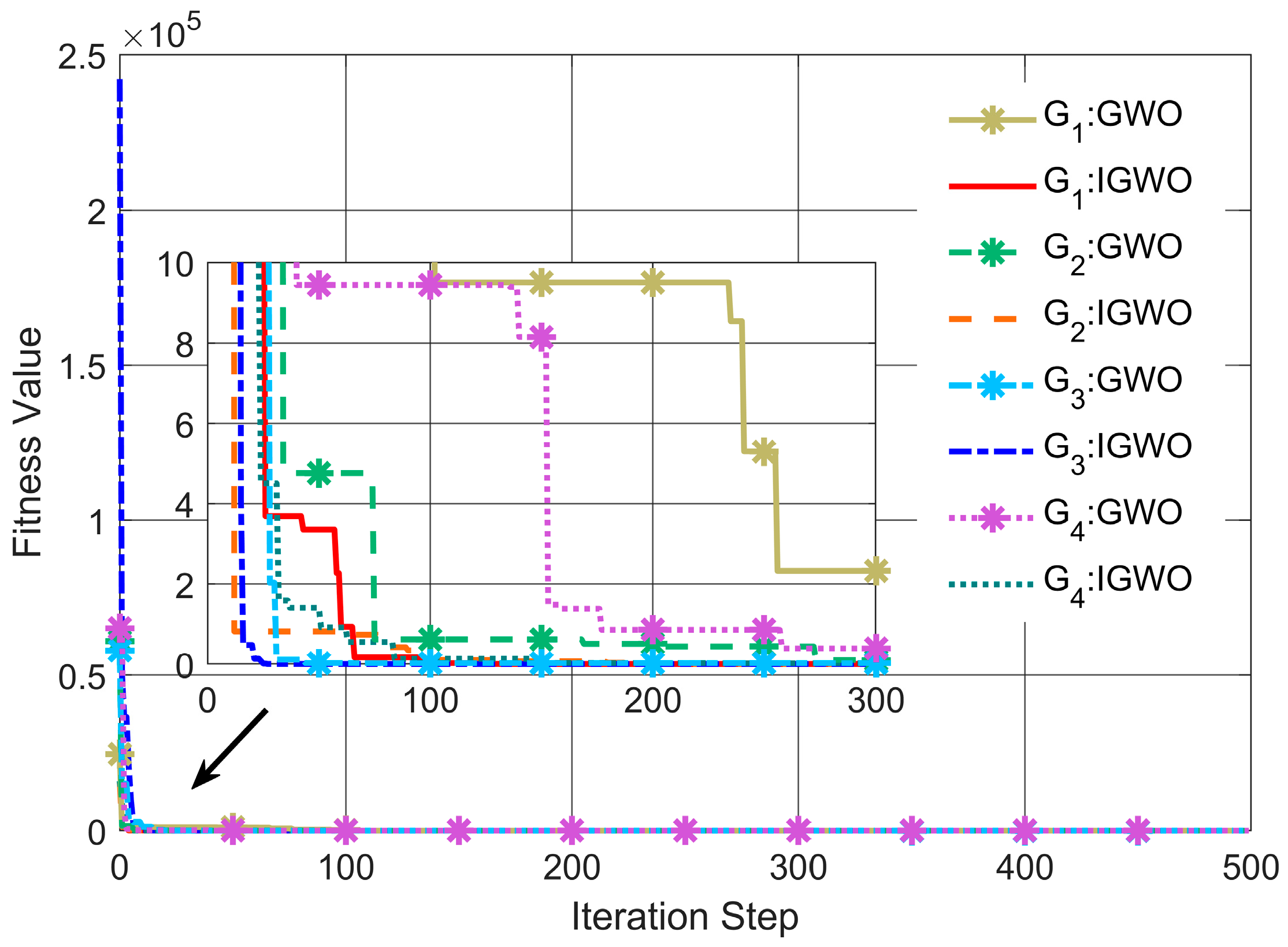
For comparison analysis,

Table 1. Comparison of calculation results using GWO and IGWO.

Algorithm	Type	R1 (m)	R2 (m)	Fitness
GWO	G1	118.03	191.65	5.5 × 10−2
	G2	228.96	289.51	6.4 × 10−3
	G3	150.68	200.14	2.1 × 10−3
	G4	102.49	152.85	5.5 × 10−2
IGWO	G1	100.02	191.65	4.7 × 10−7
	G2	289.05	289.80	9.1 × 10−5
	G3	150.13	200.57	4.6 × 10−7
	G4	113.32	148.09	5.4 × 10−3

lists the detailed numerical results, including the characteristics radii in the adjustment and circling phases, as well as the optimal fitness value, obtained under identical conditions using the standard GWO method. The results indicate that the characteristic parameters obtained by both methods are in close agreement. As depicted by the fitness curves in Figure 17, the IGWO method exhibits faster convergence across all four configurations, achieving a fitness value below 0.1 within the first 100 iterations and demonstrating a superior convergence rate.

Under the operational conditions depicted in Figure 16, a clockwise adjustment turn requires significant yaw control effort. Consequently, this maneuver results in additional height loss, thereby reducing the available margin for final landing adjustments. In contrast, trajectories G₁ and G₂ facilitate a quicker transition to the straight glide phase. Between these planning results, trajectory G₂ is selected as the nominal reference. This selection is primarily based on its larger turning radius, which allows the parafoil to maintain a stable spiral descent during the circling phase with minimal control actuation, enhancing robustness against wind uncertainties.

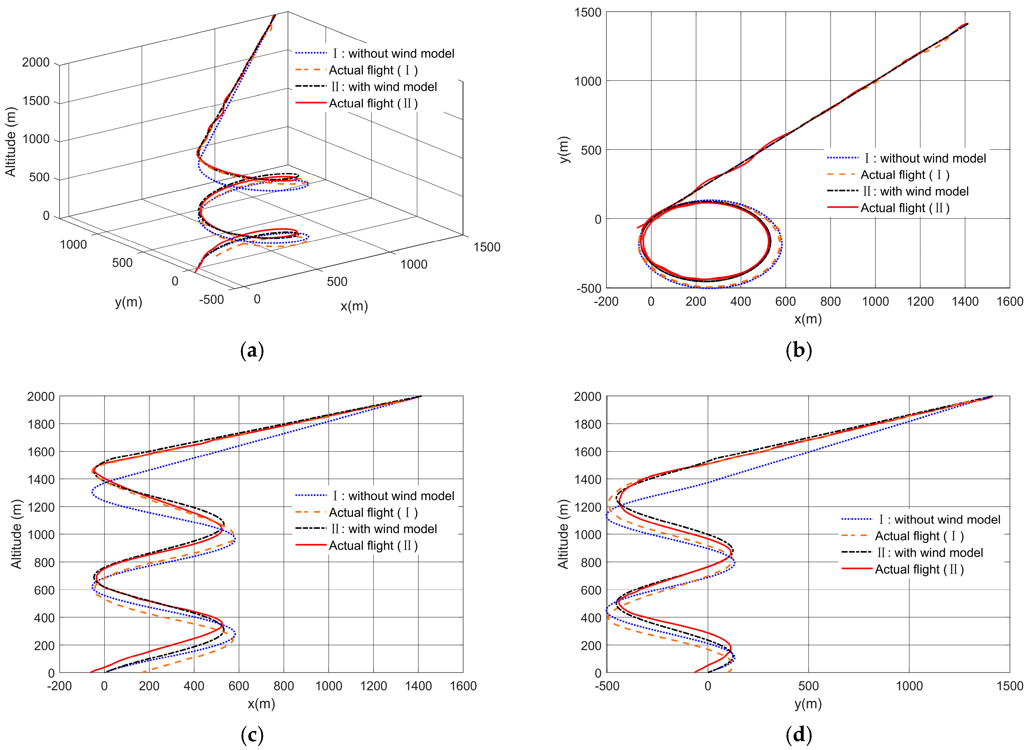
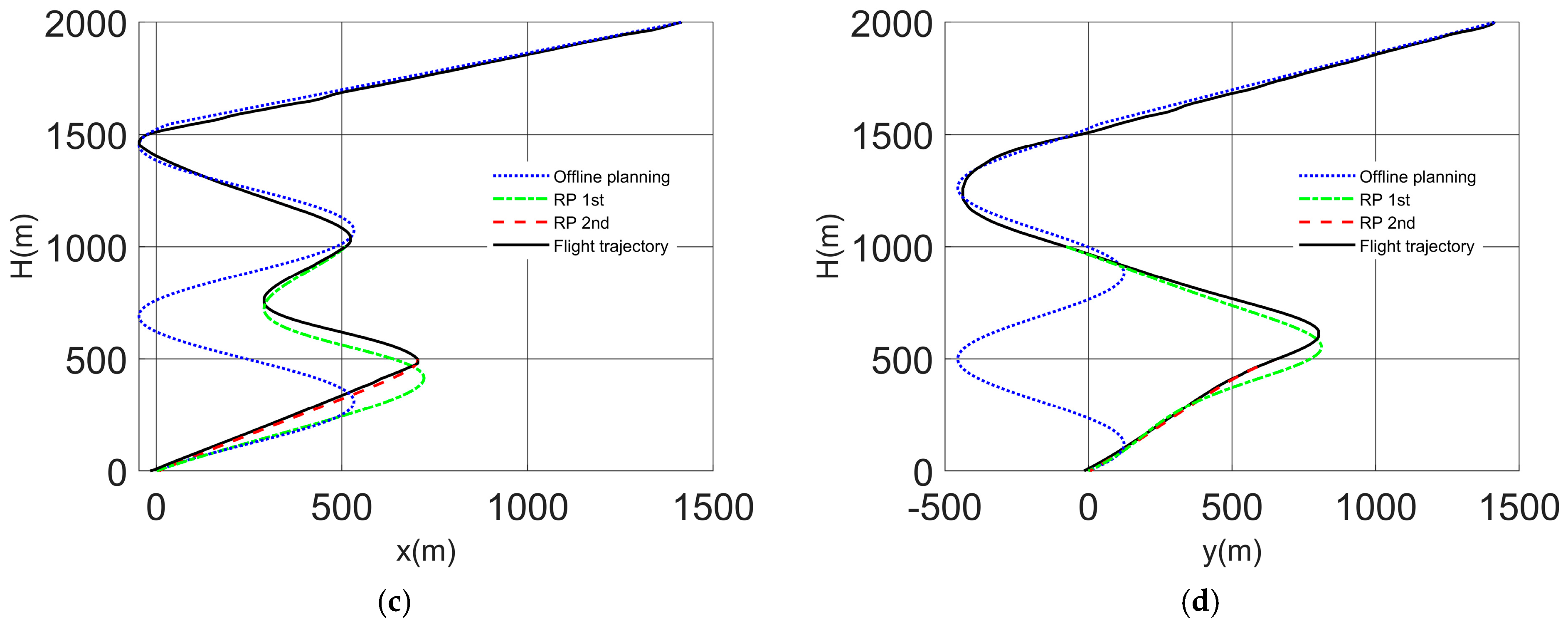
To quantitatively analyze the wind impact, two specific trajectories are planned using the IGWO method: Trajectory I is optimized for wind-free conditions, while Trajectory II accounts for a realistic wind field. The flight simulation results comparing the two guidance trajectories are presented in Figure 18. Analysis of the horizontal motion in Figure 18b confirms that the parafoil’s heading effectively tracks both reference trajectories. However, significant differences emerge in flight accuracy. For Trajectory I, the simulation reveals a consistent deviation from actual flight data. The glide ratio is overestimated in the straight phase but underestimated in the circling phase. This mismatch leads to an accumulated height error of 156 m as shown in Figure 18c, ultimately resulting in a premature touchdown with a landing position error of (168.95, 97.11) m.

In contrast, Trajectory II, which incorporates a wind model, demonstrates superior performance and a much closer match to actual flight data. The maximum height error is mitigated to approximately 56 m during the circling phase. Consequently, the final landing error is substantially reduced to (−62.09, −66.69) m. Furthermore, the tracking errors throughout the flight exhibit smaller fluctuations, indicating enhanced robustness provided by the wind-model-based design.

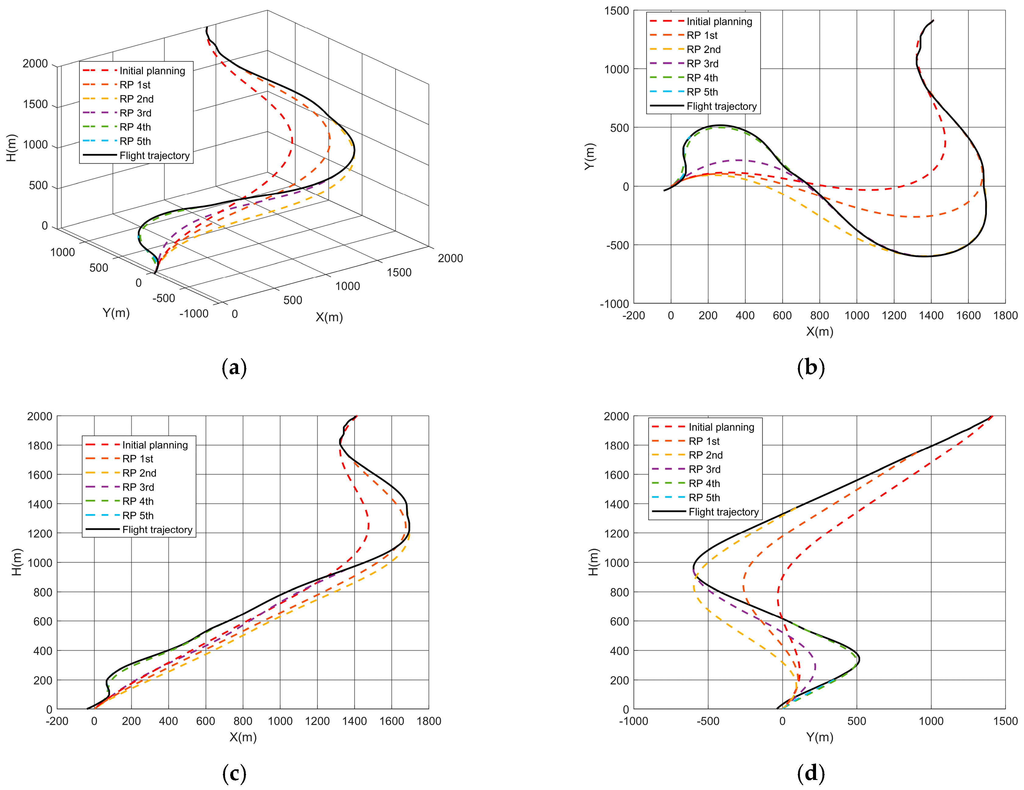
To contrast with the offline layered planning strategy, a simulation employing only DRP is conducted under identical conditions. As shown in Figure 19, the parafoil is released from the initial position (1414.2, 1414.2, −2000) m with a yaw angle of 228.14 degrees. The initial trajectory is generated using the APSM. During the flight, the guidance trajectory is sequentially updated at heights of 1749.2 m, 1373.1 m, 954.2 m, 583.6 m, and 247.3 m. Through these five trajectory updates, the final landing error is (−39.9, −38.2) m. This result indicates that DRP is more beneficial for landing precision than the offline layered planning strategy. It is also noted that a considerable horizontal maneuvering range is required to dissipate the redundant height.

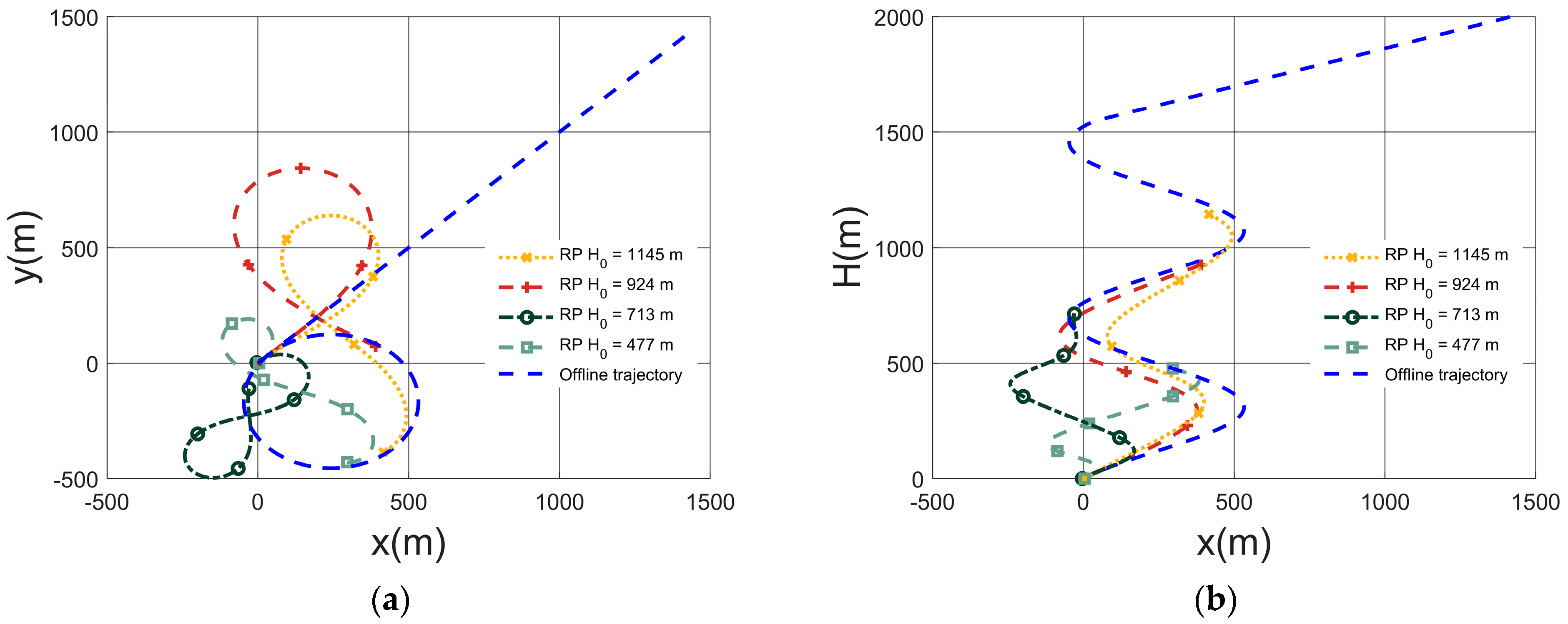
To enhance airdrop accuracy, online trajectory adjustment simulations are performed under the same conditions. The parafoil initially follows the offline trajectory II until reaching a predetermined height, at which point the reference trajectory is updated by the RP process. The parafoil then tracks the newly generated trajectory to landing. Figure 20 illustrates several replanned trajectories initiated from initial RP heights H₀ along the original path. The corresponding planning parameters, including computation time and the modified average glide ratio, are listed in

Table 2. Planning parameters for different RP height points.

RP Height	1145 m	924 m	713 m	477 m
Calculation Time	4.26 s	1.67 s	2.15 s	1.11 s
Average Glide Ratio	2.32	2.39	2.43	2.58

.

The results demonstrate that the required planning time decreases as the parafoil descends, due to the reduction in the search space as the remaining flight distance shortens. Additionally, the glide ratio gradually increases during the final phase of flight, resulting from the decrease in wind speed at lower heights.

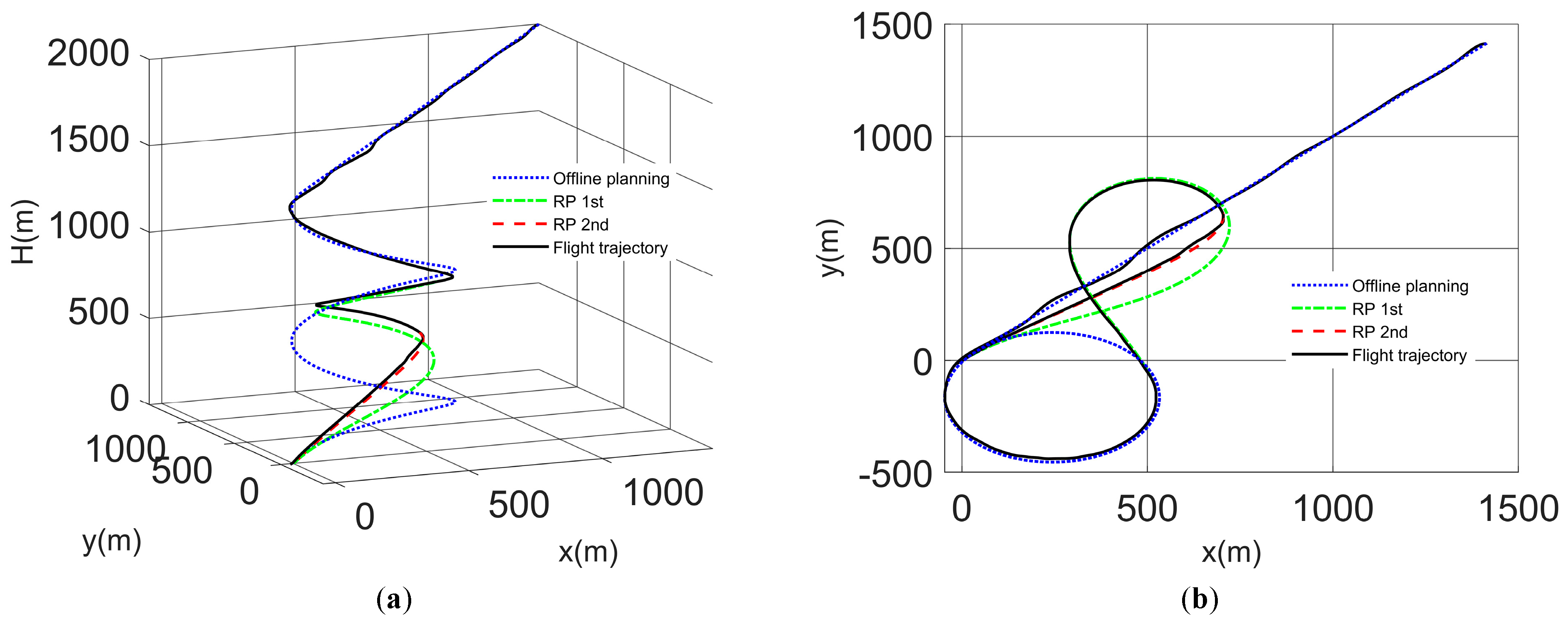
A single RP maneuver is insufficient to effectively cover the remainder of the flight, especially when initiated at higher heights. Therefore, a simulation featuring a two-stage dynamic updates strategy is conducted. As illustrated in Figure 21, the first online trajectory is planned at a height of 1000 m to replace the original offline reference trajectory. When the parafoil descends to 500 m, a second updated trajectory is planned, replacing the initial RP trajectory.

By initiating each replanning cycle from the parafoil’s current position and state, the system effectively resets the accumulated tracking error from the previous flight phase. This results in an adjusted trajectory that is more closely aligned with the parafoil’s actual glide capabilities and the prevailing environmental conditions. The final landing point error is (−16.58, −15.29) m. The parafoil touches down with a yaw angle of −145.83 degrees, which is a deviation of 11.77 degrees from the expected −134.06 degrees. Nevertheless, the landing accuracy is significantly improved compared to simply tracking the static offline trajectory.

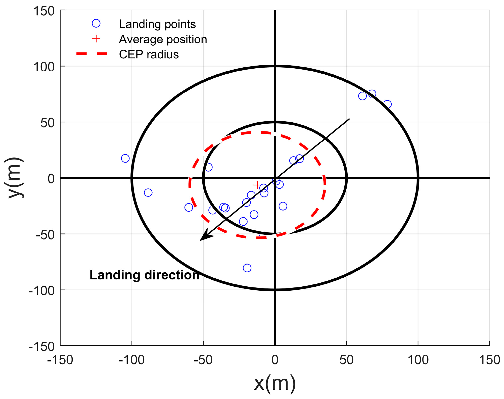
The wind field comprises a mean component, characterized by low-frequency variations predictable via wind models, and a turbulent component. The turbulent component is modeled as a random process with defined statistical properties. To assess the robustness of the dynamic planning algorithm against wind uncertainty, a Monte Carlo simulation is conducted. In each simulation, a gust-type perturbation is modeled as a maximum deviation of ±10% around a baseline wind value, in order to assess the algorithm’s robustness under varying stochastic wind conditions.

A total of 23 airdrop experiments are conducted, each incorporating two RP updates. The distribution of landing points relative to the target is shown in Figure 22. The results indicate that the majority of landing points fall within the desired 100 m error radius. The average landing position is (−12.28, −6.29) m, indicating a consistent bias to the southwest of the target, and the circular error probable (CEP) is calculated to be 47.21 m. Furthermore, the landing points are distributed along the expected landing direction, passing through the target. These data support the robustness of the DRP in achieving landing accuracy within approximately 100 m of the target under a wind environment.

4.3. Airdrop Flight Experiment

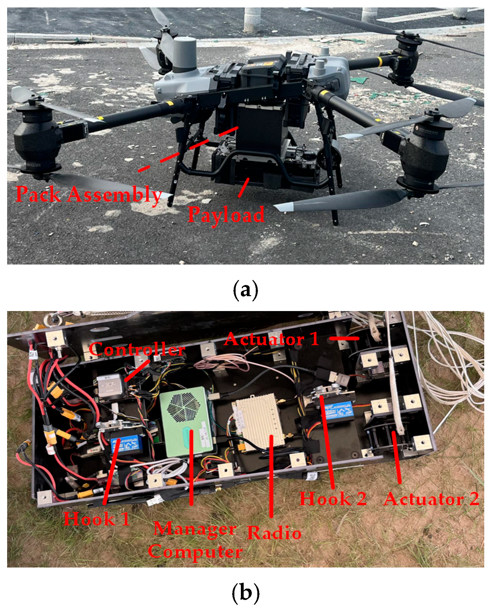
An airdrop experiment utilizing the DRP system was carried out from a height of approximately 700 m. The tested system consists of a parafoil with an area of 10 m² and a mass of 2.9 kg, carrying a 10 kg payload. The flight management computer integrated within the 10 kg payload is built around an Allspark2-x86 single-board computer (AMOVLAB, Chengdu, China), equipped with a 4.2 GHz quad-core Intel Core i7-1165G7 processor (Intel Corporation, Santa Clara, CA, USA) and 16 GB of LPDDR4 RAM. As shown in Figure 23a, the canopy is packed within a deployment box mounted beneath the fuselage. The payload is connected to the UAV by two release hooks. The payload is equipped with a flight manager computer that issues guidance commands, as shown in Figure 23b. These commands are executed by a controller, which actuates the control surfaces via steering lines for trajectory control. The controller actuates two actuators to pull down the trailing-edge steering lines and control flight. A telemetry data link transmits real-time flight data to the ground monitoring station.

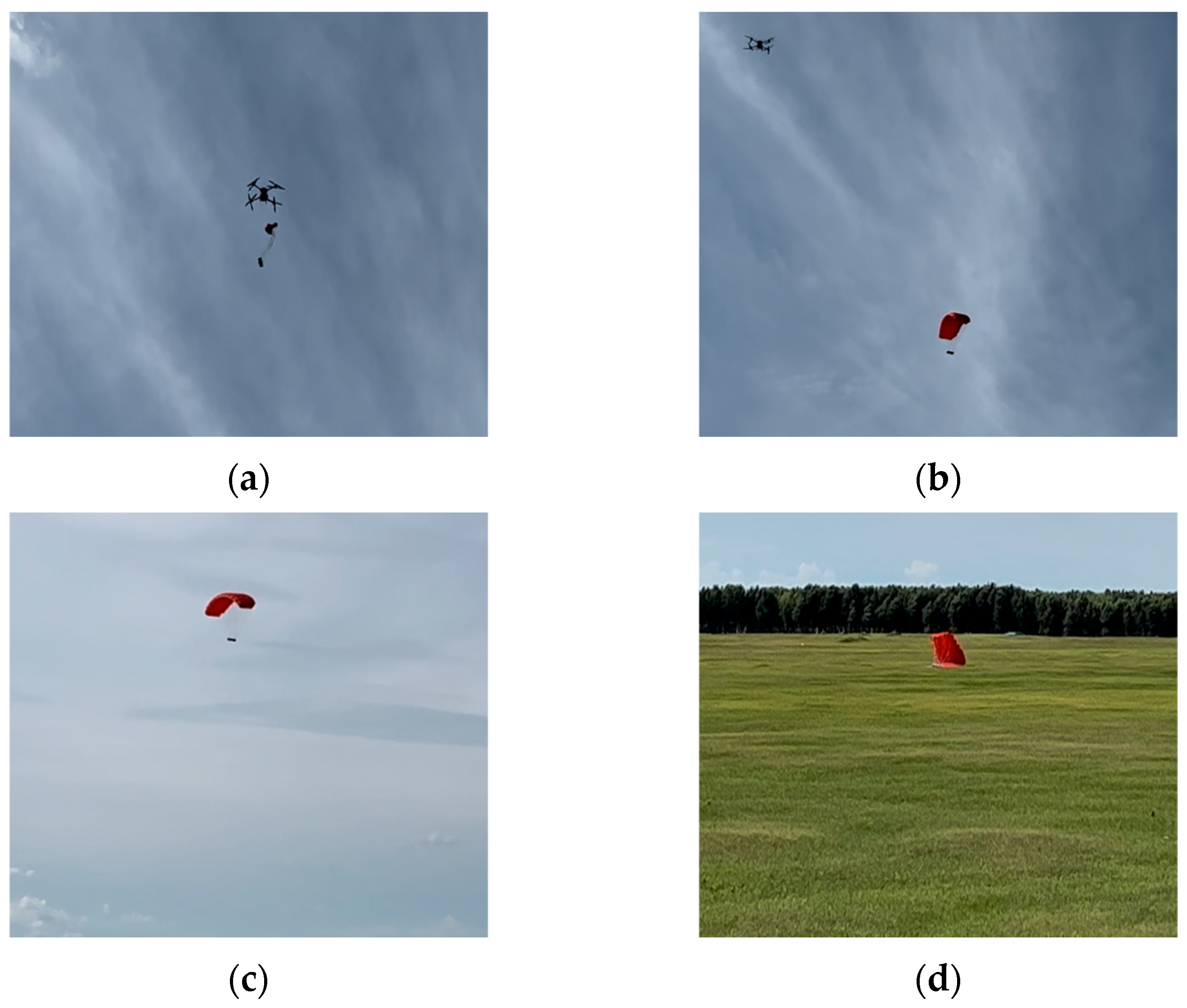
During the test, ground-level wind conditions were southerly at around 2 m/s. The parafoil was released from the UAV at an initial position of (266.84, −98.82, −685.52) m in the ground coordinate frame, with a heading of 148.7 degrees. The designated landing target was set at the coordinate origin (0, 0, 0) m, aligned with a prescribed landing direction of 180 degrees due south. As illustrated in Figure 24, an airdrop mission comprises several sequential phases. During the initial deployment phase, the release mechanism is activated, and the payload extracts the parafoil canopy from the pack assembly under gravity. The canopy then undergoes critical inflation. Following successful inflation, the system enters the stable gliding phase, where the fully inflated parafoil achieves steady flight. Subsequently, during the homing phase, the parafoil follows a planned path toward the target through a series of guidance-controlled turning maneuvers. Finally, at a specified height, a symmetric trailing-edge deflection is commanded to initiate a flared landing. This maneuver is designed to reduce both forward and descent velocity for a safe touchdown.

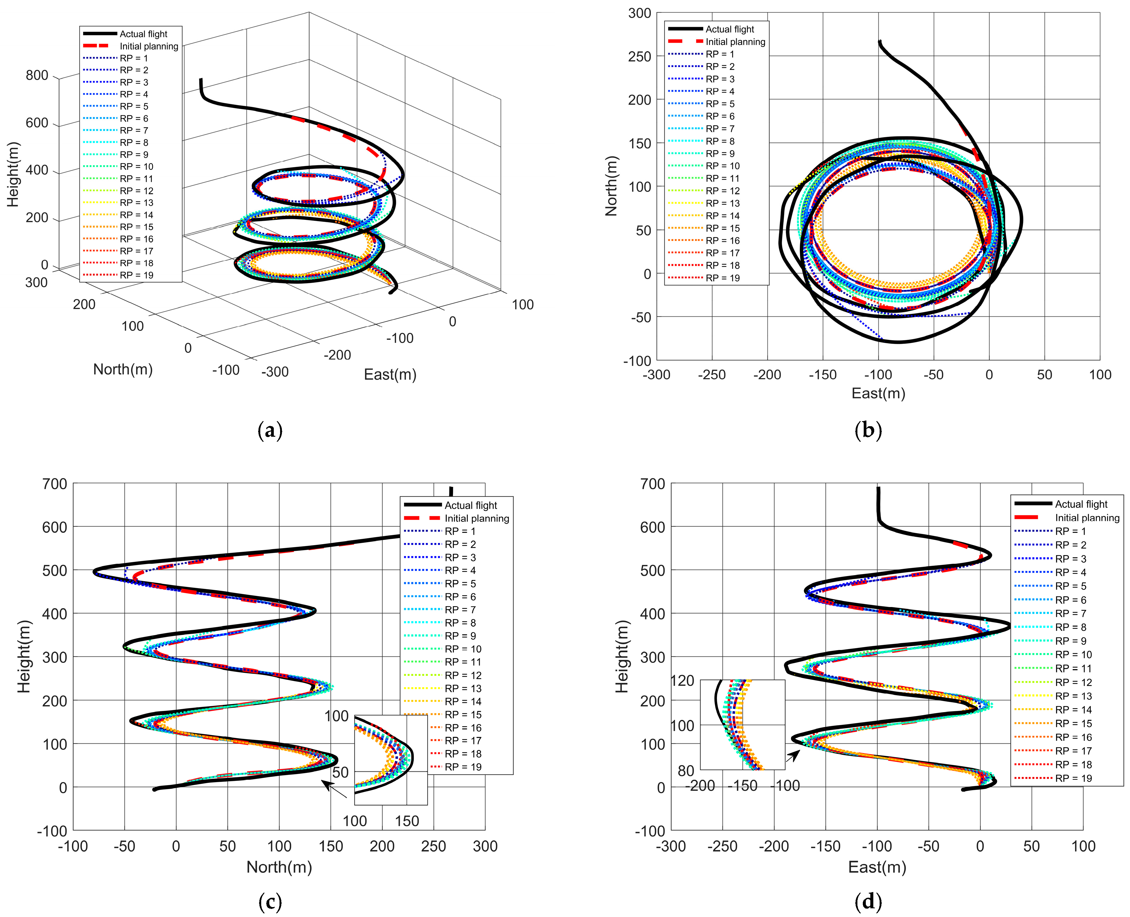
As illustrated in Figure 25, the parafoil first tracked an initial reference trajectory beginning with a height of 562.93 m, which was subsequently replaced by successively replanned trajectories. For practical implementation, the trajectory was iteratively refined through a series of bounded adjustments. Throughout the flight, a total of 19 updates were performed. During the initial flight, the parafoil exhibited a higher glider ratio than that of the reference trajectory. The onboard flight controller is only activated after the parafoil is released and achieves a steady gliding state, in order to avoid unnecessary control surface deflections during the transient deployment and inflation phase. Consequently, the comparison data between expected and actual states is calculated and sampled from the moment the controller is engaged. Therefore, the initial sampled data in the controlled flight phase naturally begins at a lower height than the original airdrop release point.

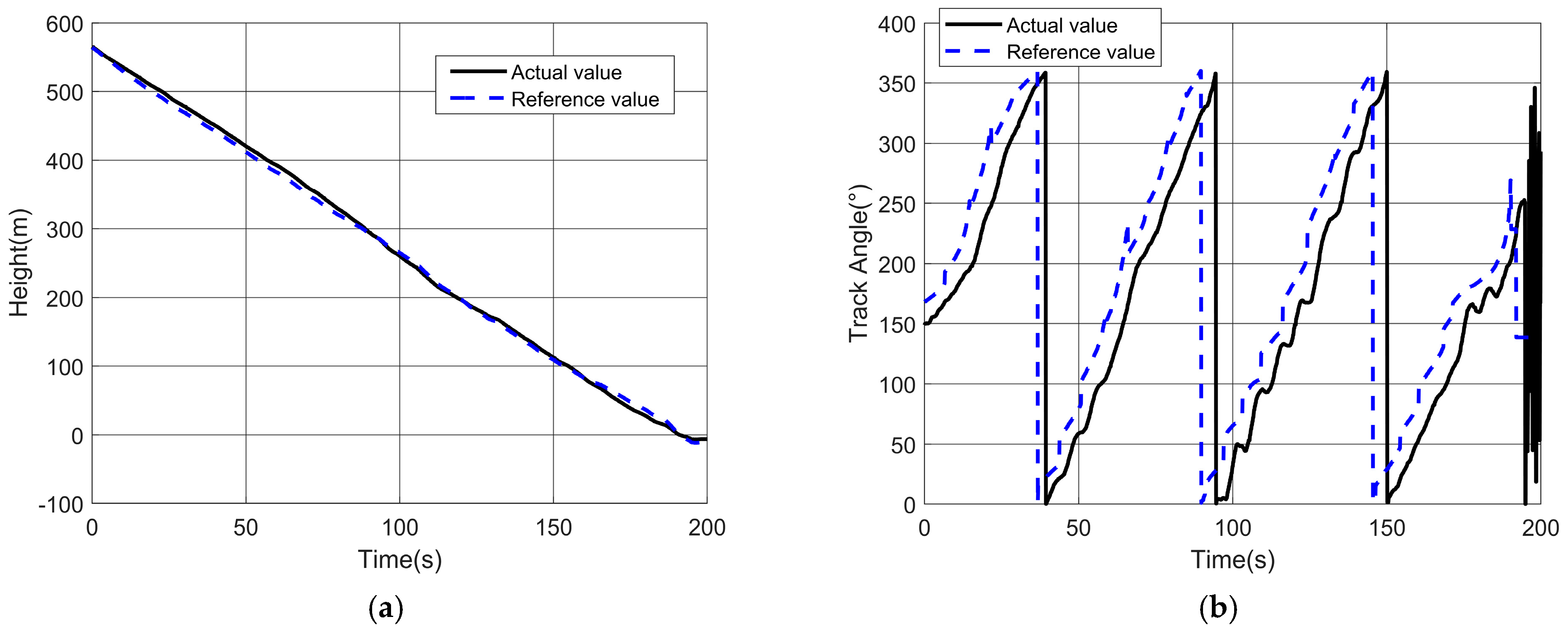
As shown in Figure 26a, the parafoil consistently flew ahead of the reference trajectory until t = 88 s. Consequently, subsequent dynamic adjustments were designed to extend the horizontal travel distance in order to dissipate the resulting height surplus. Between t = 88 s and t = 160 s, the height error between the actual position and the reference trajectory oscillated within a range of ±5.6 m. After t = 160 s, as the parafoil turned into the headwind landing direction, a larger height error of 9.3 m was rapidly introduced. This error was subsequently corrected during the final landing phase. Figure 26b presents a comparison between the actual and expected track angles. The results indicate that the tracking performance is generally satisfactory, with the actual trajectory effectively following the expected command. A sluggish response is observed in the directional motion, characterized by a time delay. This delay primarily stems from the aerodynamic response inertia inherent to the parafoil system. To compensate, a height advance of 10 m is applied for triggering waypoint switches. This provides the system with the additional time and spatial margin required to execute turn commands, thereby mitigating the adverse effects induced by the response delay. The application of the DRP strategy effectively compensates for this latency, thereby enhancing landing precision. The parafoil ultimately touched down at a horizontal position of (−20.96, −16.89) m relative to the target.

5. Conclusions

This paper proposes a combined homing method that integrates segmental and dynamic planning. Initially, the parafoil is guided toward the target using an offline trajectory. Subsequently, the terminal trajectory is planned online based on real-time conditions. The following conclusions are drawn from the results of flight simulations and experiments:

(1)

By incorporating the wind prediction model, the planned multi-phase trajectory aligns more closely with the actual motion characteristics than ignoring wind effects. Following the layered homing strategy, the parafoil is ensured to be guided into the target zone well for landing.

(2)

The replanning optimization is performed and resolved quickly through time and space normalizations. Dynamic terminal adjustment effectively compensates for the deviation caused by external disturbances. In addition, the online updated trajectory is better suited for the remaining flight, which is beneficial for landing precision.

(3)

Results show that the DRP method satisfies gliding performance requirements for underactuated parafoil systems in windy conditions. It reduces the flight control workload, ensuring high precision in airdrop operations despite external wind disturbances.

The research in this paper benefits the parafoil autonomous homing technology in complex environments. Future work will focus on integrating higher-fidelity turbulence and gust models to test the algorithm under conditions that more closely resemble severe, realistic flight environments, and engineering validation of the proposed method through flight tests in mountain environments.

References

1. Baiocco, P. Overview of reusable space systems with a look to technology aspects. Acta Astronaut. 2021, 189, 10–25. [Google Scholar] [CrossRef] [Scilit]
2. Dek, C.; Overkamp, J.L.; Toeter, A.; Hoppenbrouwer, T.; Slimmens, J.; van Zijl, J.; Rossi, P.A.; Machado, R.; Hereijgers, S.; Kilic, V.; et al. A recovery system for the key components of the first stage of a heavy launch vehicle. Aerosp. Sci. Technol. 2020, 100, 105778. [Google Scholar] [CrossRef] [Scilit]
3. de Lange, M.H.; Verhoek, C.; Preda, C.; Tóth, R. LPV modeling of the atmospheric flight dynamics of a generic parafoil return vehicle. IFAC-PapersOnLine 2022, 55, 37–42. [Google Scholar] [CrossRef] [Scilit]
4. Salzman, O.; Halperin, D. Asymptotically near-optimal RRT for fast, high-quality motion planning. IEEE Trans. Robot. 2016, 32, 473–483. [Google Scholar] [CrossRef] [Scilit]
5. Lee, I.R.; Choi, Y.S.; Lim, M.G.; Woo, J.W.; Kim, C.J. Guidance and control for autonomous emergency landing of the rotorcraft using the incremental backstepping controller in 3-dimensional terrain environments. Aerosp. Sci. Technol. 2023, 132, 108051. [Google Scholar] [CrossRef] [Scilit]
6. Alnuaimi, M.; Perhinschi, M. Performance comparison of clothoid and dubins path generation algorithms. In Proceedings of the AIAA Aviation 2022 Forum, Chicago, IL, USA, 27 June–1 July 2022. [Google Scholar] [CrossRef] [Scilit]
7. Arslan, Ö.; Tiemessen, A. Adaptive Bézier degree reduction and splitting for computationally efficient motion planning. IEEE Trans. Robot. 2022, 38, 3655–3674. [Google Scholar] [CrossRef] [Scilit]
8. Fossen, T.I.; Pettersen, K.Y.; Galeazzi, R. Line-of-sight path following for dubins paths with adaptive sideslip compensation of drift forces. IEEE Trans. Control Syst. Technol. 2015, 23, 820–827. [Google Scholar] [CrossRef] [Scilit]
9. Wang, J.; Sun, H.; Sun, J. An optimal multiphase homing method of parafoil system based on genetic algorithm. In Proceedings of the 2022 7th International Conference on Robotics and Automation Engineering, Singapore, 18–20 November 2022. [Google Scholar] [CrossRef] [Scilit]
10. Wang, Y.; Yang, C.; Yang, H. Neural network-based simulation and prediction of precise airdrop trajectory planning. Aerosp. Sci. Technol. 2022, 120, 107302. [Google Scholar] [CrossRef] [Scilit]
11. Fowler, L.; Rogers, J. Bézier Curve Path Planning for Parafoil Terminal Guidance. J. Aerosp. Inf. Syst. 2014, 11, 300–315. [Google Scholar] [CrossRef] [Scilit]
12. Rademacher, B.J.; Lu, P.; Strahan, A.L.; Cerimele, C.J. In-flight trajectory planning and guidance for autonomous parafoils. J. Aeros. Inf. Syst. 2009, 32, 1697–1712. [Google Scholar] [CrossRef] [Scilit]
13. Yang, L.; Zhao, X.; Gu, F.; He, Y. Multi-phase homing optimal control for parafoil system. In Proceedings of the 2016 IEEE International Conference on Robotics and Biomimetics, Qingdao, China, 3–7 December 2016; pp. 1343–1348. [Google Scholar] [CrossRef] [Scilit]
14. Eberhart, R.; Kennedy, J. A new optimizer using particle swarm theory. In IEEE MHS’95, Proceedings of the Sixth International Symposium on Micro Machine and Human Science, Nagoya, Japan, 4–6 October 1995; IEEE: New York, NY, USA, 1995; pp. 39–43. [Google Scholar] [CrossRef] [Scilit]
15. Dorigo, M.; Briattari, M.; Blum, C.; Clerc, M.; Stützle, T.; Winfield, A. Ant colony optimization and swarm intelligence. In Proceedings of the 6th International Conference, ANTS 2008, Brussels, Belgium, 22–24 September 2008. [Google Scholar] [CrossRef] [Scilit]
16. Mirjalili, S.; Mirjalili, S.M.; Lewis, A. Grey wolf optimizer. Adv. Eng. Softw. 2014, 69, 46–61. [Google Scholar] [CrossRef] [Scilit]
17. An, K.; Guo, Z.Y.; Xu, X.P.; Huang, W. A framework of trajectory design and optimization for the hypersonic gliding vehicle. Aerosp. Sci. Technol. 2020, 106, 106110. [Google Scholar] [CrossRef] [Scilit]
18. Zhou, C.; He, L.; Yan, X.; Meng, F.; Li, C. Active-set pseudospectral model predictive static programming for midcourse guidance. Aerosp. Sci. Technol. 2023, 134, 108137. [Google Scholar] [CrossRef] [Scilit]
19. Zhu, H.; Sun, Q.; Tao, J.; Chen, Z.; Dehmer, M.; Xie, G. Flexible modeling of parafoil delivery system in wind environments. Commun. Nonlinear Sci. 2022, 108, 106210. [Google Scholar] [CrossRef] [Scilit]
20. Chiel, B.S.; Dever, C. Autonomous parafoil guidance in high winds. J. Guid. Control Dynam. 2015, 38, 963–969. [Google Scholar] [CrossRef] [Scilit]
21. Luders, B.; Ellertson, A.; How, J.P.; Sugel, I. Wind uncertainty modeling and robust trajectory planning for autonomous parafoils. J. Guid. Control Dynam. 2016, 39, 1614–1630. [Google Scholar] [CrossRef] [Scilit]
22. Ward, M.; Costello, M. Adaptive glide slope control for parafoil and payload aircraft. J. Guid. Control Dynam. 2013, 36, 1019–1034. [Google Scholar] [CrossRef] [Scilit]
23. Ward, M.; Culpepper, S.; Costello, M. Parafoil control using payload weight shift. J. Aircraft 2014, 51, 204–215. [Google Scholar] [CrossRef] [Scilit]
24. Gavrilovski, A.; Ward, M.; Costello, M. Parafoil control authority with upper-surface canopy spoilers. J. Aircraft 2012, 49, 1391–1397. [Google Scholar] [CrossRef] [Scilit]
25. Slegers, N.; Yakimenko, O.A. Terminal guidance of autonomous parafoils in high wind-to-airspeed ratios. Proc. Inst. Mech. Eng. Part G J. Aerosp. Eng. 2011, 225, 336–346. [Google Scholar] [CrossRef] [Scilit]
26. Li, Y.; Pang, B.; Wei, C.; Cui, N.; Liu, Y. Online trajectory optimization for power system fault of launch vehicles via convex programming. Aerosp. Sci. Technol. 2020, 98, 105682. [Google Scholar] [CrossRef] [Scilit]
27. Yu, W.; Chen, W. Entry guidance with real-time planning of reference based on analytical solutions. Adv. Space Res. 2015, 55, 2325–2345. [Google Scholar] [CrossRef] [Scilit]
28. Miao, X.; Cheng, L.; Zhang, Z.; Li, J.; Gong, S. Convex optimization for post-fault ascent trajectory replanning using auxiliary phases. Aerosp. Sci. Technol. 2023, 138, 108336. [Google Scholar] [CrossRef] [Scilit]
29. Bonaccorsi, G.; Quadrelli, M.B.; Braghin, F. Dynamic programming and model predictive control approach for autonomous landings. J. Guid. Control Dynam. 2022, 45, 2164–2173. [Google Scholar] [CrossRef] [Scilit]
30. Yakimenko, O.A. Precision Aerial Delivery Systems: Modeling Dynamics, and Control; American Institute of Aeronautics and Astronautics, Inc.: Reston, VA, USA, 2015; Volume 248, pp. 11–16. [Google Scholar] [CrossRef] [Scilit]
31. Yang, H.; Song, L.; Chen, W. Research on parafoil stability using a rapid estimate model. Chin. J. Aeronaut. 2017, 30, 1670–1680. [Google Scholar] [CrossRef] [Scilit]
32. Li, B.; He, Y.; Han, J.; Xiao, J. A new modeling scheme for powered parafoil unmanned aerial vehicle platforms: Theory and experiments. Chin. J. Aeronaut. 2019, 32, 2466–2479. [Google Scholar] [CrossRef] [Scilit]
33. Ochi, Y. Modeling and simulation of flight dynamics of a relative-roll-type parafoil. In Proceedings of the AIAA SciTech 2020 Forum, Orlando, FL, USA, 6–10 January 2020. [Google Scholar] [CrossRef] [Scilit]
34. Song, Z.; Li, Y.; Yu, L.; Li, X. Coupling model analysis for aerodynamic performance of parafoil with maneuvers. J. Beijing Univ. Aeronaut. Astronaut. 2024. (Published Online). (In Chinese) [Google Scholar] [CrossRef]
35. Wachlin, J.; Ward, M.; Costello, M. In-canopy sensors for state estimation of precision guided airdrop systems. Aerosp. Sci. Technol. 2019, 90, 357–367. [Google Scholar] [CrossRef] [Scilit]
36. Deng, Y.; Zhang, X.; Zhang, G. Line-of-sight-based guidance and adaptive neural path-following control for sailboats. IEEE J. Ocean. Eng. 2020, 45, 1177–1189. [Google Scholar] [CrossRef] [Scilit]
37. Yan, L.; Song, Y.; Wang, H.; Shi, Z. Dynamics modeling and autonomous landing for flexible parafoil-vehicle multibody system. IEEE Access 2023, 11, 43945–43961. [Google Scholar] [CrossRef] [Scilit]
38. Guo, B.; Bacha, S.; Alamir, M.; Mohamed, A.; Boudinet, C. LADRC applied to variable speed micro-hydro plants: Experimental validation. Control Eng. Pract. 2019, 85, 290–298. [Google Scholar] [CrossRef] [Scilit]
39. Song, Y.; Ma, G.; Tian, L.; Zhao, N.; Lu, X. Numerical investigations of precise wind field in main landing area during the landing phase of “shen zhou” series spacecraft mission. Aerospace 2023, 10, 37. [Google Scholar] [CrossRef] [Scilit]
40. Nadimi-Shahraki, M.H.; Taghian, S.; Mirjalili, S. An improved grey wolf optimizer for solving engineering problems. Expert Syst. Appl. 2020, 166, 113917. [Google Scholar] [CrossRef] [Scilit]
Figure 1. Work frame of the automatic following system for the parafoil airdrop.
Aerospace 13 00276 g001
Figure 2. The simplified schematic diagram of a parafoil system. The red dashed line indicates the xc-zc plane. The yellow dashed line indicates the projection line of the canopy airspeed vector.
Aerospace 13 00276 g002
Figure 3. Schematic diagram of the line-of-sight guidance law for parafoil flight: (a) Heading channel. (b) Height channel.
Aerospace 13 00276 g003
Figure 4. Flight performance of the parafoil system during Test A: (a) Comparison between the actual horizontal motion trajectory and the expected airdrop path. (b) Time histories of the horizontal speed, vertical speed, and glide ratio.
Aerospace 13 00276 g004
Figure 5. Flight performance of the parafoil system during Test B: (a) Comparison between the actual horizontal motion trajectory and the expected airdrop path. (b) Time histories of the horizontal speed, vertical speed, and glide ratio.
Aerospace 13 00276 g005
Figure 7. Trajectory profile configurations with different rotation directions, where line colors denote distinct flight phases: pink (direction adjustment), green (straight glide), yellow (height reduction via circling), and blue (flared landing): (a) G1: n1 = −1, n2 = 1. (b) G2: n1 = −1, n2 = −1. (c) G3: n1 = 1, n2 = −1. (d) G4: n1 = 1, n2 = 1.
Aerospace 13 00276 g007aAerospace 13 00276 g007b
Figure 8. Key node positions with different bitangents: (a) Point P is located between the two circles. (b) Point P lies on one side of the two circles.
Aerospace 13 00276 g008
Figure 9. Comparison of wind fields between the predicted model and realistic observations.
Aerospace 13 00276 g009
Figure 10. The hierarchical planning process from global multiple-phase trajectory generation to local dynamic planning.
Aerospace 13 00276 g010
Figure 11. Schematic diagram of the decomposition of ground velocity into airspeed and wind velocity components.
Aerospace 13 00276 g011
Figure 12. Planned trajectories for variable wind direction based on APSM.
Aerospace 13 00276 g012
Figure 13. Comparison of the actual flight trajectory and the planned trajectories under a wind speed of 1 m/s from 315 degrees: (a) Horizontal plane projection. (b) Vertical height profile.
Aerospace 13 00276 g013
Figure 14. Comparison of the actual flight trajectory and the planned trajectories under a wind speed of 3 m/s from 180 degrees: (a) Horizontal plane projection. (b) Vertical height profile.
Aerospace 13 00276 g014
Figure 15. Comparison of the actual flight trajectory and the planned trajectories under a wind speed of 5 m/s from 360 degrees: (a) Horizontal plane projection. (b) Vertical height profile.
Aerospace 13 00276 g015
Figure 16. Results of planned trajectories for different configurations through the IGWO method.
Aerospace 13 00276 g016
Figure 17. Iteration convergence curves from GWO and IGWO.
Aerospace 13 00276 g017
Figure 18. Comparison of the planned trajectories with and without the wind model to the actual flight paths: (a) Three-dimensional trajectory. (b) xy plane. (c) xz plane. (d) yz plane.
Aerospace 13 00276 g018
Figure 19. The flight simulation only using DRP without layered planning: (a) Three-dimensional trajectory. (b) xy plane. (c) xz plane. (d) yz plane.
Aerospace 13 00276 g019
Figure 20. RP trajectories from different height points along the offline trajectory: (a) Horizontal plane. (b) Vertical plane.
Aerospace 13 00276 g020
Figure 21. Comparison between the two-stage RP trajectories and the flight trajectory: (a) Three-dimensional trajectory. (b) xy plane. (c) xz plane. (d) yz plane.
Aerospace 13 00276 g021aAerospace 13 00276 g021b
Figure 22. Distribution of landing points relative to the target.
Aerospace 13 00276 g022
Figure 23. The UAV-parafoil airdrop test system (Note: The non-English characters visible on some components are printed labels or marks used in the experiments): (a) The connection between the UAV and the parafoil. (b) The equipment composition of the test system in the payload.
Aerospace 13 00276 g023
Figure 24. Sequential phases of a parafoil airdrop mission from a UAV. The process includes: (a) Deployment phase. (b) Stable gliding phase. (c) Homing phase. (d) Flared landing phase.
Aerospace 13 00276 g024
Figure 25. Comparison between the planned trajectories and the realistic flight: (a) Three-dimensional trajectory. (b) xy plane. (c) xz plane. (d) yz plane.
Aerospace 13 00276 g025
Figure 26. Comparison between flight states and reference states: (a) Height. (b) Track angle.
Aerospace 13 00276 g026