Mesh-Agnostic Model for the Prediction of Transonic Flow Field of Supercritical Airfoils

Abstract

Mesh-agnostic models have advantages in processing flow field data with various topologies and densities, and they can easily incorporate partial differential equations. Beyond physics-informed neural networks, mesh-agnostic models have been studied for data-driven predictions of simple flows. In this study, a data-driven mesh-agnostic model is proposed to predict the transonic flow field of various supercritical airfoils. The model consists of two subnetworks, i.e., ShapeNet and HyperNet. ShapeNet is an implicit neural representation used to predict spatial bases of the flow field. HyperNet is a simple neural network that determines the weights of these bases. The input of ShapeNet is extended to ensure accurate prediction for different airfoil geometries. To reduce overfitting while capturing shock waves and boundary layers, a multi-resolution ShapeNet combining two activation functions is proposed. Additionally, a physics-guided loss function is proposed to enhance accuracy. The proposed model is trained and tested on various supercritical airfoils under different free-stream conditions. Results show that the model can effectively utilize airfoil samples with different grid sizes and distributions, and it can accurately predict the shock wave and boundary layer velocity profile. The proposed mesh-agnostic model can be used as a decoder in any conventional models, contributing to their application in complex and three-dimensional geometries.

1. Introduction

The aerodynamic optimization of modern civil aircraft remains an expensive and time-consuming process. Despite the availability of high-performance computing (HPC) resources and efficient computational fluid dynamics (CFD) solvers, the design cycle for three-dimensional (3D) wings is still lengthy. Over the past few decades, machine learning has been extensively developed and investigated for aerodynamic design [1]. It has been utilized for geometric modeling [2] and filtering [3], the prediction of performance and flow fields [4], and machine-learning-assisted optimization [1], etc.

Flow fields constitute the physical basis of aerodynamic characteristics and contain substantially richer information than integrated performance coefficients alone. In practice, designers evaluate candidate configurations and refine designs based on both aerodynamic coefficients and salient flow field features [5]. Consequently, accurate flow field prediction is a key enabler for machine-learning-assisted aerodynamic optimization. A variety of learning models have been investigated for fast and accurate flow prediction, including convolutional neural networks (CNNs) [6,7], variational autoencoders (VAEs) [8,9], and generative adversarial networks (GANs) [10,11]. However, most existing studies focus on two-dimensional (2D) flows around airfoils.

Predicting 3D flow fields for complex geometries faces several major challenges: (1) the curse of dimensionality; (2) high sampling and training costs; and (3) difficulty of data formatting. Firstly, three-dimensional aircraft have many geometric design variables as model inputs, and their flow field also contains millions of data points, which makes the model significantly bigger and more difficult to train. Secondly, such a big model requires a lot of samples for training. It makes the computational cost of data sampling unaffordable because 3D CFD simulations are much more expensive than 2D simulations. Therefore, many of the studies on 3D flows focus on the prediction of a fixed geometry under different flight conditions [12,13,14], or the prediction of similar geometries [15]. Recently, transfer learning has been explored to reduce sampling and training costs across different geometries and flight conditions [16]. Multi-fidelity and multi-resolution approaches have also been studied to further reduce computational expenses [17,18]. In these scenarios, the diversity of data sources and formats introduces additional challenges for machine learning.

Data formatting presents a further difficulty for flows around complex geometries in both 2D and 3D. Machine learning, especially deep learning, usually requires samples to have the same data format so that they can be assembled into tensors [19]. However, the topology, size, and distribution of CFD meshes can be very different for different configurations, free-stream conditions, and solvers. Structured meshes make it easier to maintain the same topology, size, and distribution for similar geometries, e.g., different 2D airfoils or different 3D wings in similar planforms and configurations. However, the mesh topology and quality may be poor for complex geometries, which can degrade both CFD accuracy and machine learning performance. Unstructured meshes are easy to generate, but it is difficult to maintain the same size and distribution for different geometries. Therefore, the raw CFD data is usually transformed into structured data formats for machine learning. For example, flow fields are usually interpolated into images, i.e., uniform Cartesian structured data representations, for training [6,7,10,11,12,20]. However, images provide low resolution near geometry boundaries, so the prediction accuracy of boundary layers is often unsatisfactory. Single-block structured meshes can also be transformed via coordinate mappings, which can maintain the resolution of boundary layers [8,9,15]. However, such data transformations are not always applicable to complex geometries or three-dimensional aircraft configurations.

Mesh-agnostic learning methods aim to circumvent these issues by avoiding reliance on a specific mesh topology or connectivity. Representative examples include implicit neural representations (INRs) [21], graph CNNs [22], and PointNet [23], which have demonstrated the potential in handling unstructured data. Moreover, INR-based frameworks such as physics-informed neural networks (PINNs) [24] and deep operator networks (DeepONets) [25] can incorporate physical constraints or governing partial differential equations (PDEs) directly into the learning process. Consequently, DeepONets have attracted increasing interest as physics-guided models for aerodynamic design in recent years [26,27,28]. Nevertheless, challenges remain for mesh-agnostic approaches in rapidly predicting transonic flow fields across different geometries, including (1) the determination of geometry boundaries and (2) balancing the different resolutions required by flow structures, such as the free stream, boundary layers, and shock waves.

In this work, a mesh-agnostic model is proposed for the fast prediction of various supercritical airfoils under different free-stream conditions. The model employs an INR to represent spatial bases of the flow field, enabling the use of physics-guided loss functions that enhance shock wave resolution. A hypernetwork [29] is further introduced to map parameter inputs (e.g., free-stream conditions and airfoil geometric parameters) to the corresponding flow field bases.

The novelty of this work can be summarized in three aspects. First, an implicit, mesh-agnostic decoder is developed to predict full-field, multi-variable transonic RANS solutions rather than scalar quantities or surface data commonly considered in previous DeepONet-based studies. Second, a geometry-aware input encoding based on the logarithm of the wall distance is introduced, enabling consistent representation of boundary layer physics across different airfoil geometries. Third, a multi-resolution ShapeNet combined with a physics-guided loss is proposed to effectively capture both smooth flow regions and localized high-gradient structures such as shock waves.

The remainder of this paper is organized as follows. First, the sample generation and preparation procedure for supercritical airfoils is described. Next, the architecture of the proposed mesh-agnostic model is presented. Techniques to improve boundary layer and shock wave prediction, as well as strategies to suppress far-field overfitting, are then introduced. Finally, the model is evaluated on different airfoil geometries and free-stream conditions.

2. Sample Preparation

2.1. Supercritical Airfoil Database

Supercritical airfoils are generated using the class shape transformation (CST) method [30]. In this study, a ninth-order Bernstein polynomial is adopted to parameterize the shape function. The upper and lower surfaces of the airfoil are defined as:

$$y=C_{N_2}^{N_1}(x){\sum }_{i=1}^{n_{\mathrm{c}\mathrm{s}\mathrm{t}}}{c}_i{K}_i{x}^i{\left(1-x\right)}^{n-i},$$

(1)

where

$$K_i={\displaystyle \frac{n_{\mathrm{c}\mathrm{s}\mathrm{t}}!}{i!\left(n_{\mathrm{c}\mathrm{s}\mathrm{t}}-i\right)!}}, C_{N_2}^{N_1}\left(x\right)=x^{N_1}{\left(1-x\right)}^{N_2}, N_1=0.5, N_2=1.0.$$

(2)

For the ninth-order Bernstein polynomial, $n_{\mathrm{c}\mathrm{s}\mathrm{t}}=10$ and $x\in \left[0,1\right]$. Thus, there are 20 CST parameters ${\left\{c_i\right\}}_{i=1}^{20}$ that define the geometry of the unit-chord-length airfoil.

A C–H-type grid is generated for airfoils with a unit chord length, and the open-source solver CFL3D [31] is used for the CFD simulations. The first-layer wall-normal spacing is specified such that $\Delta y^{+}$ remains below 1 for all cases. A total of 301 grid points are distributed along the airfoil surface. The simulations are performed using the MUSCL reconstruction with Roe’s approximate Riemann solver; the governing equations are advanced using the lower–upper symmetric Gauss–Seidel (LU-SGS) method, and turbulence closure is provided by the $k–\omega$ shear-stress-transport (SST) model within the Reynolds-averaged Navier–Stokes (RANS) framework. The CFL number is set to 2.0, and each case is marched for 8000 iterations. The Reynolds number is fixed at ${10}^7$.

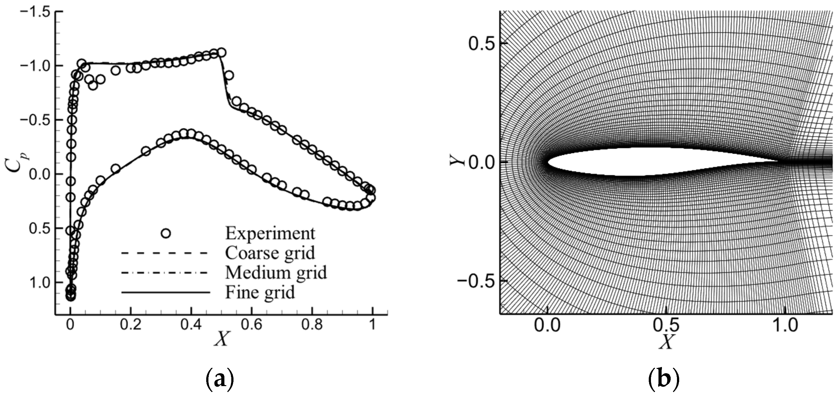
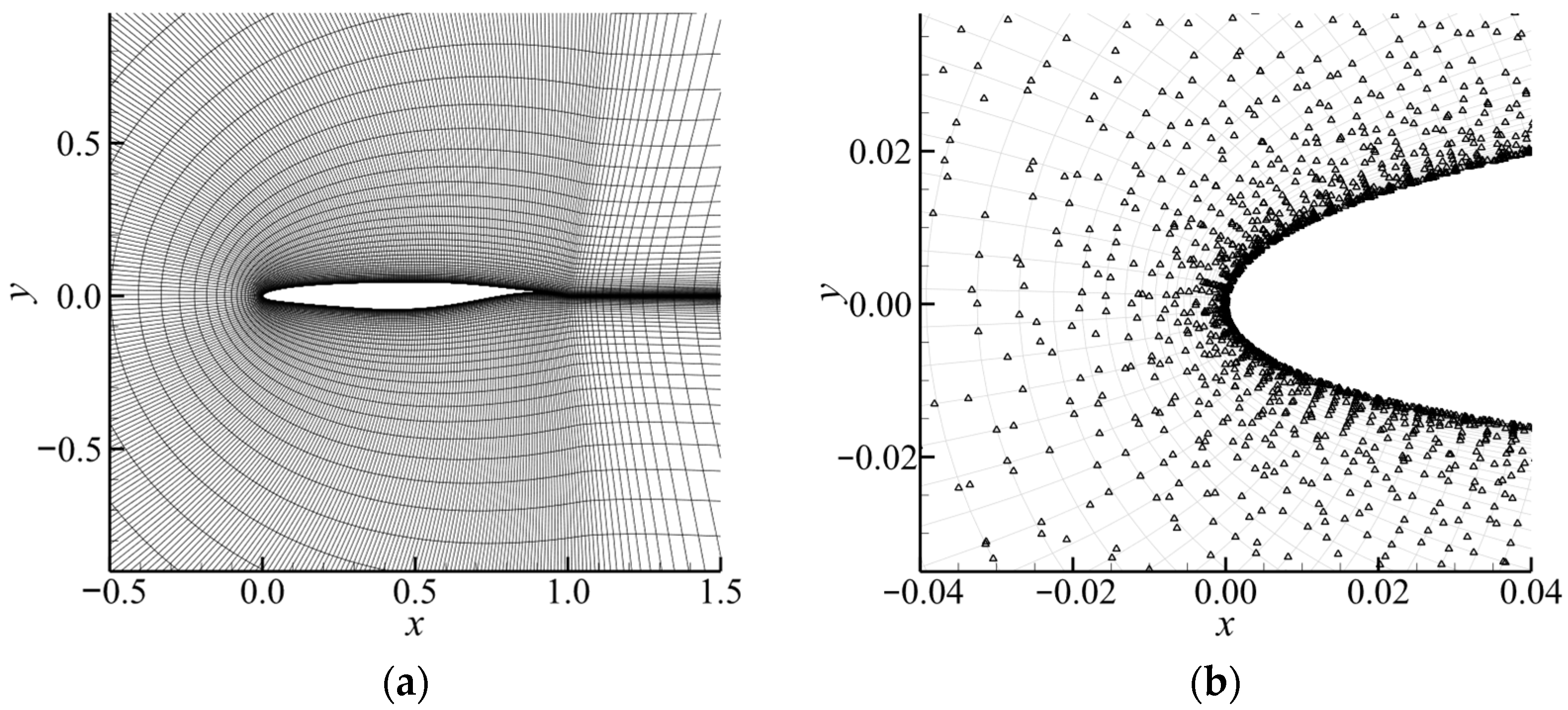
Figure 1a shows the experimental pressure coefficient ($C_p$) distributions of an RAE2822 airfoil compared with the CFD results of different grid sizes. The free-stream Mach number ($M_{\mathrm{\infty }}$) is 0.725, the Reynolds number ($Re$) based on the unit chord length is $6.5\times {10}^6$, and the angle of attack ($\mathrm{A}\mathrm{o}\mathrm{A}$) is 2.55 degrees. The three grids have sizes of 20,000, 40,000, and 80,000, respectively. All grids can achieve a similar $C_p$ resolution. The medium grid is shown in Figure 1b, which is employed in this paper.

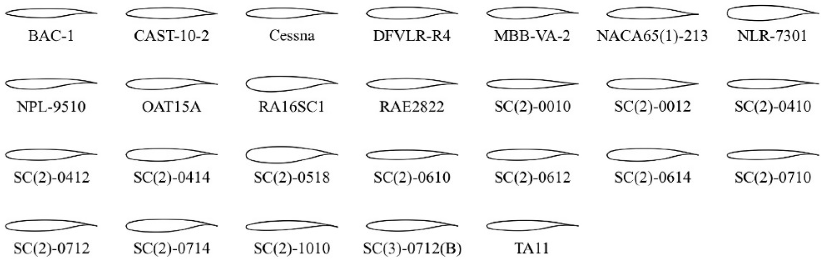
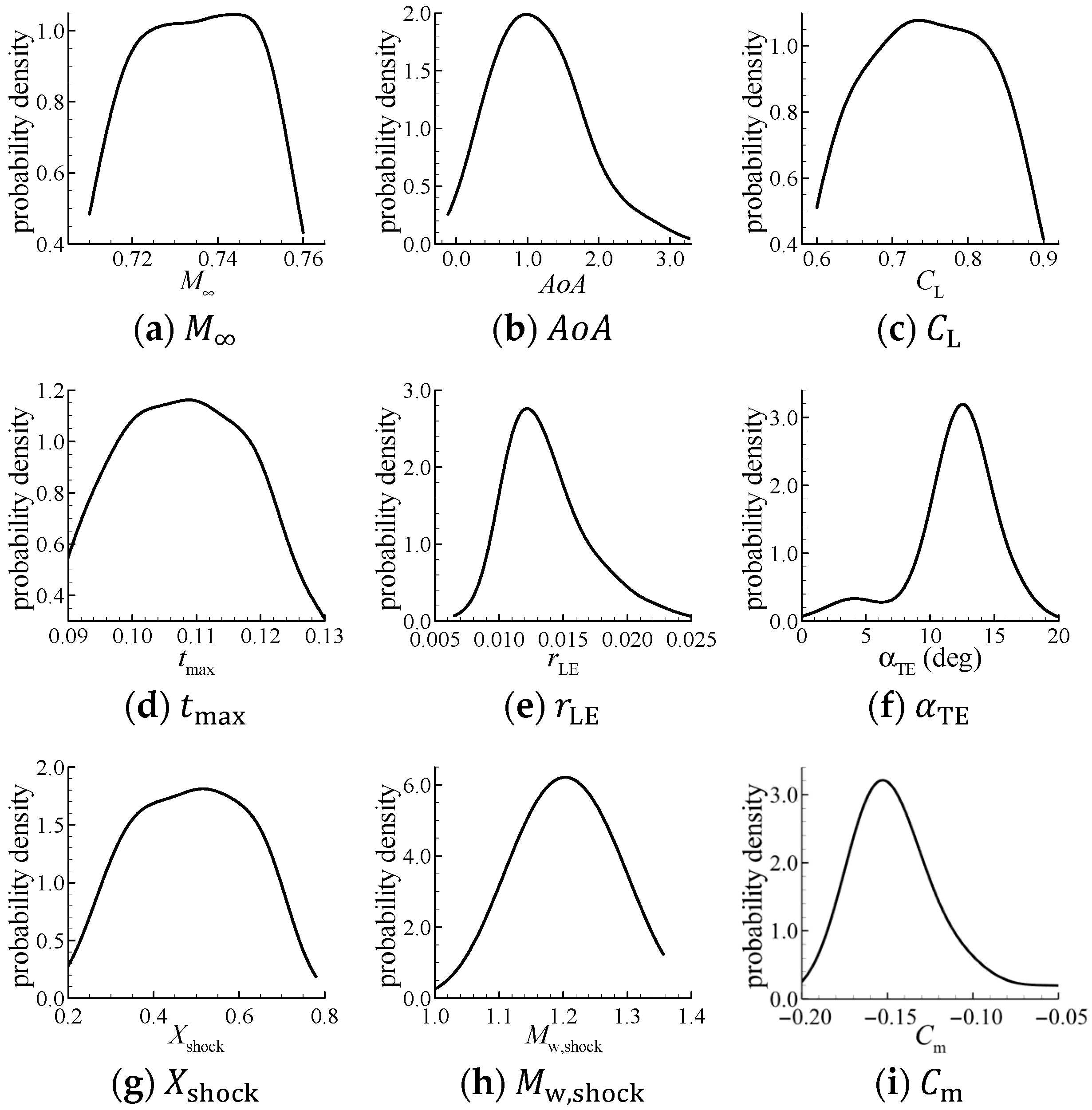
A customized supercritical-airfoil database is used in this study. The database is constructed to cover a broad range of free-stream conditions, airfoil geometries, and shock wave characteristics relevant to transonic civil transport aircraft [28]. It contains 2500 airfoils, including 35 classic supercritical airfoils (Figure 2), 100 conventional airfoils from the University of Illinois Urbana–Champaign (UIUC) low-speed airfoil database [32], and additional supercritical airfoils sampled using the output-space sampling method [5]. The sample density distributions are shown in Figure 3.

Figure 3a–c illustrate the diversity of free-stream conditions, including the free-stream Mach number $M_{\mathrm{\infty }}$, angle of attack ($\mathrm{A}\mathrm{o}\mathrm{A}$, deg), and lift coefficient $C_L$. Figure 3d–f summarize the geometric diversity in terms of the maximum relative thickness $t_{\mathrm{m}\mathrm{a}\mathrm{x}}$, leading-edge radius $r_{\mathrm{L}\mathrm{E}}$, and trailing-edge slope angle ${\alpha }_{\mathrm{T}\mathrm{E}}$ (deg). The camber-related diversity is implicitly captured through the varying CST parameters. The diversity of camber distributions in the dataset can be qualitatively observed from the baseline airfoil samples shown in Figure 2. Figure 3g–i characterize the flow field diversity using the shock location $X_{\mathrm{s}\mathrm{h}\mathrm{o}\mathrm{c}\mathrm{k}}$, the pre-shock wall Mach number $M_{\mathrm{w},\mathrm{s}\mathrm{h}\mathrm{o}\mathrm{c}\mathrm{k}}$, and the moment coefficient $C_{\mathrm{m}}$. Here, the wall Mach number is computed from the surface pressure coefficient $C_p$ and the free-stream Mach number based on an isentropic relation [33]. The database is randomly split into a training set and a testing set containing 2300 and 200 airfoils, respectively.

All samples in the present database are computed at Re = 10⁷ to represent typical high-Re civil-aircraft transonic conditions. Consequently, the current model is validated for variations in geometry and free-stream conditions at a fixed Reynolds number; generalization across Reynolds numbers is not assessed in this work.

2.2. Data Preparation

The C–H-type grid for each airfoil is generated using an in-house elliptic grid-generation code. The CFD solution is stored at the grid points, including density $\rho$, velocities $u$ and $v$, pressure $p$, and Mach number $M$. Figure 4a shows an example grid for a representative supercritical airfoil. Because the same grid size and distribution settings are used throughout the sampling process, the grid point distribution is largely consistent across all airfoil cases. This consistency is advantageous for mesh-based machine learning models. However, it provides information only at discrete grid points and does not explicitly represent the regions between them. Consequently, using only the default grid point distribution may encourage overfitting in mesh-agnostic models.

To mitigate overfitting and to better leverage the strengths of mesh-agnostic models, the raw solution on the C–H-type grid is interpolated onto randomly sampled points, as illustrated in Figure 4b. For each airfoil case, one point is uniformly sampled within each grid cell, and the flow variables at that location are obtained using dual-linear Coons transfinite (bilinear) interpolation:

$$v^{\prime }=\left(1-r_1\right)\left(1-r_2\right)v_0+r_1\left(1-r_2\right)v_1+\left(1-r_1\right)r_2{v}_3+r_1{r}_2{v}_2,$$

(3)

where $v^{\prime }$ denotes the interpolated value and $v_i\left(i=0,1,2,3\right)$ are the values at the four corner nodes of a quadrilateral cell. The quadrilateral grid cell is defined by four vertices, 0, 1, 2, and 3, and $r_1$ and $r_2$ are the ratios of the interpolated point in edge 01 and 02, respectively.

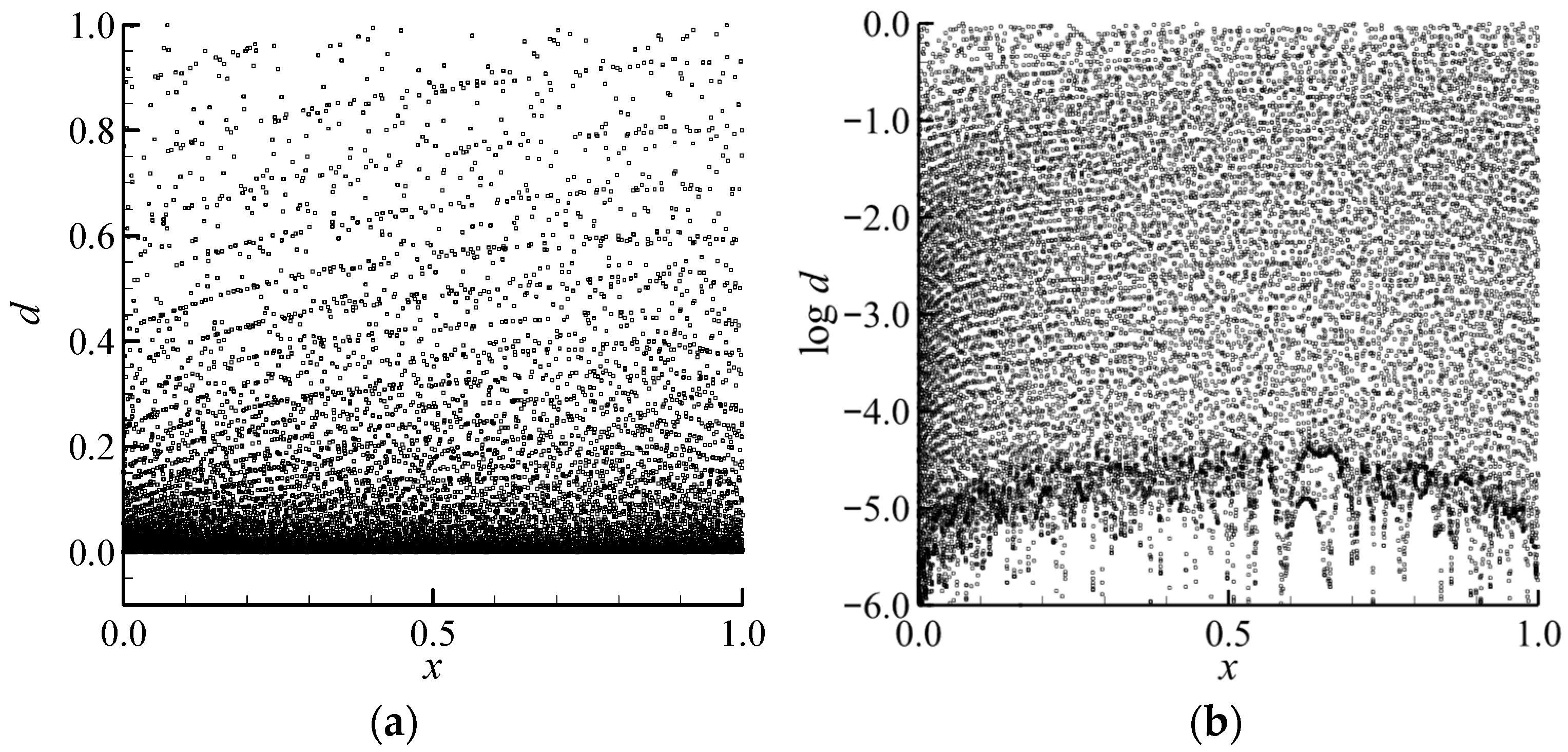
On the other hand, transonic flows over supercritical airfoils require non-uniformly distributed grid points to properly resolve near-wall behavior (e.g., the logarithmic law of the wall), which can pose challenges for model training. Because the Reynolds number is fixed at ${10}^7$ for all samples, the first-layer height corresponding to $y^{+}\approx 1$ is on the order of ${10}^{-6}$. Figure 5a shows the distribution of the randomly sampled points with respect to their distance to the airfoil surface, $d$, and their $x$-coordinate. Figure 5b replots the same distribution using $\log d$ versus $x$, which helps alleviate overfitting by improving the effective sampling in the near-wall region. Moreover, the distance to the airfoil surface provides additional geometric context that facilitates flow field prediction across different airfoils, as discussed in Section 4.2.

The sampling procedure is summarized in Algorithm 1. Each sampled point is represented as:

$${\mathit{p}}_i={\left[x,y,d,\rho ,u,v,p,M\right]}^T.$$

For each flow field solution containing $n_{\mathrm{grid}}$ grid points, $n_{\mathrm{point}}$ data points are randomly sampled. In this study, $n_{\mathrm{grid}}=\mathrm{32,481}$ and $n_{\mathrm{point}}=\mathrm{20,000}$. Consequently, the dataset comprises 50 million point samples drawn from the flow fields of 2500 airfoils. The total number of sampled points is denoted by $N_{\mathrm{point}}$.

Algorithm 1 random sampling of data points in the flow field
1:	$\mathrm{Grid} \mathrm{points} \mathrm{of} \mathrm{one} \mathrm{flow} \mathrm{field} {\mathcal{D}}_{\mathrm{g}\mathrm{r}\mathrm{i}\mathrm{d}}={\left\{{\mathit{p}}_{\mathrm{g}\mathrm{r}\mathrm{i}\mathrm{d},i}\right\}}_{i=0}^{n_{\mathrm{g}\mathrm{r}\mathrm{i}\mathrm{d}}}$;
2:	$\mathrm{for} i=1,\dots ,n_{\mathrm{g}\mathrm{r}\mathrm{i}\mathrm{d}}$ {
3:	$r_1=\mathrm{r}\mathrm{a}\mathrm{n}\mathrm{d}(0,1)$$, r_2=\mathrm{r}\mathrm{a}\mathrm{n}\mathrm{d}(0,1)$;
4:	$\mathrm{Get} \mathrm{the} \mathrm{grid} \mathrm{points} {\mathit{p}}_{\mathrm{g}\mathrm{r}\mathrm{i}\mathrm{d}, i}^1$$, {\mathit{p}}_{\mathrm{g}\mathrm{r}\mathrm{i}\mathrm{d},i}^2$$\mathrm{and} {\mathit{p}}_{\mathrm{g}\mathrm{r}\mathrm{i}\mathrm{d},i}^3$$\mathrm{adjacent} \mathrm{to} \mathrm{grid} \mathrm{point} i$$({\mathit{p}}_{\mathrm{g}\mathrm{r}\mathrm{i}\mathrm{d},i}^0$);
5:	$\mathrm{Get} \mathrm{the} \mathrm{new} \mathrm{data} \mathrm{point} {\mathit{p}}_i$ by the dual-linear Coons transfinite interpolation (Equation (3));
6:	Calculate the distance to airfoil surface from the interpolated data point;
7:	};
8:	$\mathrm{Randomly} \mathrm{sample} n_{\mathrm{p}\mathrm{o}\mathrm{i}\mathrm{n}\mathrm{t}}$ data points from the interpolated data points.

3. Theoretical Methods

3.1. Data-Driven Mesh-Agnostic Model for Flow Field Prediction

The mesh-agnostic model is built upon the implicit decoder proposed in [28], which was originally developed for airfoil pressure distribution prediction and inverse design. The implicit decoder can serve as a mesh-agnostic alternative to conventional decoders in a wide range of applications, thereby offering broad applicability. In this study, it is further extended to the prediction of two-dimensional transonic viscous flow fields.

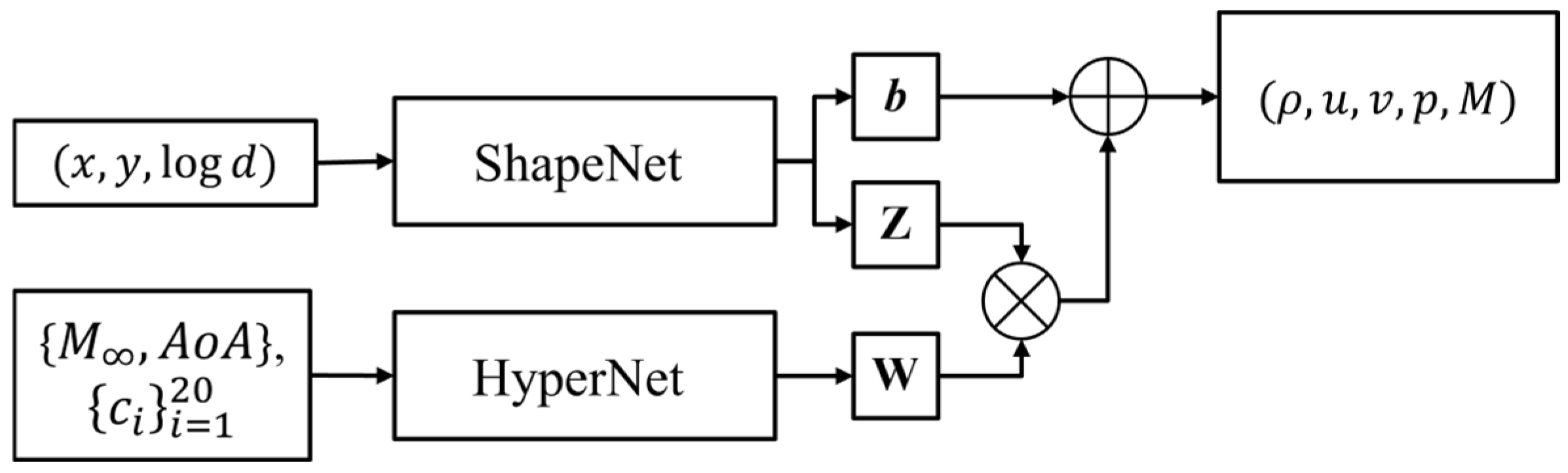
The overall architecture of the proposed flow field prediction model is illustrated in Figure 6. It consists of two subnetworks, namely ShapeNet and HyperNet. ShapeNet represents the spatial bases of the flow field: it takes the point coordinates $\mathit{x}\in {\mathrm{R}}^{n_x}$ as input and outputs the spatial bases $\mathbf{Z}\in {\mathrm{R}}^{n_{\mathrm{l}}\times n_y}$ together with an output bias $\mathit{b}\in {\mathrm{R}}^{n_y}$, where $n_x$ is the coordinate dimension, $n_y$ is the number of output variables, and $n_{\mathrm{l}}$ denotes the number of latent variables (i.e., the number of spatial bases). HyperNet predicts the weights associated with each spatial basis, $\mathbf{W}\in {\mathrm{R}}^{n_{\mathrm{l}}\times n_y}$. It takes as input the conditioning vector $\mathit{c}\in {\mathrm{R}}^{n_c}$, which includes the free-stream Mach number $M_{\mathrm{\infty }}$, angle of attack (AoA), and the CST coefficients describing the airfoil geometry. The outputs of ShapeNet and HyperNet are combined in an embedding layer via a multiplication operation:

$${\widehat{y}}_j={\sum }_{k=1}^{n_{\mathrm{l}}}{W}_{k,j}{Z}_{k,j}+b_j, j=1,\dots ,n_y,$$

(4)

where $j,k$ represent the indices of the components of vectors $\widehat{\mathit{y}}$ and $\mathit{b}$ and matrices $\mathbf{W}$ and $\mathbf{Z}$. Equation (4) shows that the output $\widehat{\mathit{y}}$ is a linear combination of the spatial bases $\mathbf{Z}$. Then, the mesh-agnostic model can be denoted by $\widehat{\mathit{y}}=\mathsf{\Phi }\left(\mathit{x}\right|\mathit{c})$. The data-driven loss function is the mean square error (MSE) of data points:

$${\mathrm{l}\mathrm{o}\mathrm{s}\mathrm{s}}_{\mathrm{M}\mathrm{S}\mathrm{E}}={\sum }_{i=1}^{N_{\mathrm{p}\mathrm{o}\mathrm{i}\mathrm{n}\mathrm{t}}}{\left[\mathsf{\Phi }\left({\mathit{x}}_i\right|{\mathit{c}}_i)-{\mathit{y}}_i\right]}^2,$$

(5)

where each data point provides a triplet $\left({\mathit{x}}_i,{\mathit{c}}_i,{\mathit{y}}_i\right)$, and $N_{\mathrm{p}\mathrm{o}\mathrm{i}\mathrm{n}\mathrm{t}}$ is the total number of data points.

To improve flow field prediction across different airfoil geometries, the logarithm of the distance to the surface, $\log d$, is included as a model input. The distance-to-surface information has been widely used in CNN-based flow field prediction models [20], typically in the form of a signed distance function (SDF). The SDF is defined as the orthogonal distance from a point $\left(x,y\right)$ to the airfoil surface, with the sign indicating whether the point lies inside or outside the solid region; this representation enables the airfoil boundary to be distinguished on Cartesian grids. In the present study, however, no training samples are taken inside the airfoil, and the SDF provides limited resolution for near-wall variations in the boundary layer. Therefore, $\log d$ is adopted as the geometric input instead.

Model parameters are optimized using the Adam optimizer [34] for up to 10,000 epochs. The learning rate is initialized at ${10}^{-3}$ and is gradually decayed to ${10}^{-6}$ during training.

3.2. Physics-Guided Loss Function to Capture Flow Structures

Transonic flows exhibit complex structures, including boundary layers, shock waves, and flow separation. This complexity leads to a multi-resolution learning problem in two respects. First, the data points are distributed non-uniformly, with substantially higher sampling density in the boundary layer region than in the outer flow. Second, shock waves introduce sharp gradients (near-discontinuities) that require higher effective resolution than smooth free-stream regions.

For the first aspect, the C–H-type grid places roughly half of the data points within the boundary layer, which may bias training and promote overfitting in the near-wall region. For the second aspect, accurately resolving shock-induced gradients typically requires additional guidance because only a limited number of samples fall in the shock region. To address these issues, identification functions for the shock wave and boundary layer regions are introduced. These functions are used to reweight point contributions in the mean squared error (MSE) loss, guiding the mesh-agnostic model to learn the multi-resolution features of the flow field.

A key advantage of the proposed mesh-agnostic formulation is that spatial derivatives can be computed directly, which enables pointwise shock identification. Accordingly, an identification function for the shock wave region is defined as:

$$r_{\mathrm{s}\mathrm{h}\mathrm{o}\mathrm{c}\mathrm{k}}=\exp \left(-{\displaystyle \frac{{\left(M-{\mu }_M\right)}^2}{2{\sigma }_M^2}}\right)/\left[1+\exp \left(2{\sigma }_{M_x}\left({\displaystyle \frac{\partial M}{\partial x}}-{\mu }_{M_x}\right)\right)\right],$$

(6)

which consists of two parts. The numerator is a Gaussian function for the Mach number, centered at ${\mu }_M=1.0$ with a standard deviation ${\sigma }_M=0.2$. It is used to identify the region where Mach number is approximately 1.0. The denominator is a Sigmoid function for the gradient of the Mach number in the $x$-direction, of which the critical value ${\mu }_{M_x}$ equals $-3.0$ and ${\sigma }_{M_x}=0.5$. It is used to identify the region where $\partial M/\partial x$ has a large negative value. An identification function for the boundary layer region is also proposed as:

$$r_{\mathrm{b}\mathrm{l}}=1/\left[1+\exp \left(10000\left({\mu }_d-d\right)\right)\right],$$

(7)

where the critical distance is ${\mu }_d=0.02$. The boundary layer region is approximated as the area where the distance to the airfoil surface is less than 0.02 chord length. Then, the weight of each data point is calculated by:

$${\lambda }_i=\min \left(\min \left(r_{\mathrm{s}\mathrm{h}\mathrm{o}\mathrm{c}\mathrm{k},i}+0.5, 1.0\right)\cdot \max \left(r_{\mathrm{b}\mathrm{l},i}, 0.02\right), 1.0\right).$$

(8)

The physics-guided data-driven loss function becomes:

$${\mathrm{l}\mathrm{o}\mathrm{s}\mathrm{s}}_{\mathrm{M}\mathrm{S}\mathrm{E}}={\sum }_{i=1}^{N_{\mathrm{p}\mathrm{o}\mathrm{i}\mathrm{n}\mathrm{t}}}{\lambda }_i{\left[\mathsf{\Phi }\left({\mathit{x}}_i\right|{\mathit{c}}_i)-{\mathit{y}}_i\right]}^2/{\sum }_{i=1}^{N_{\mathrm{p}\mathrm{o}\mathrm{i}\mathrm{n}\mathrm{t}}}{\lambda }_i.$$

(9)

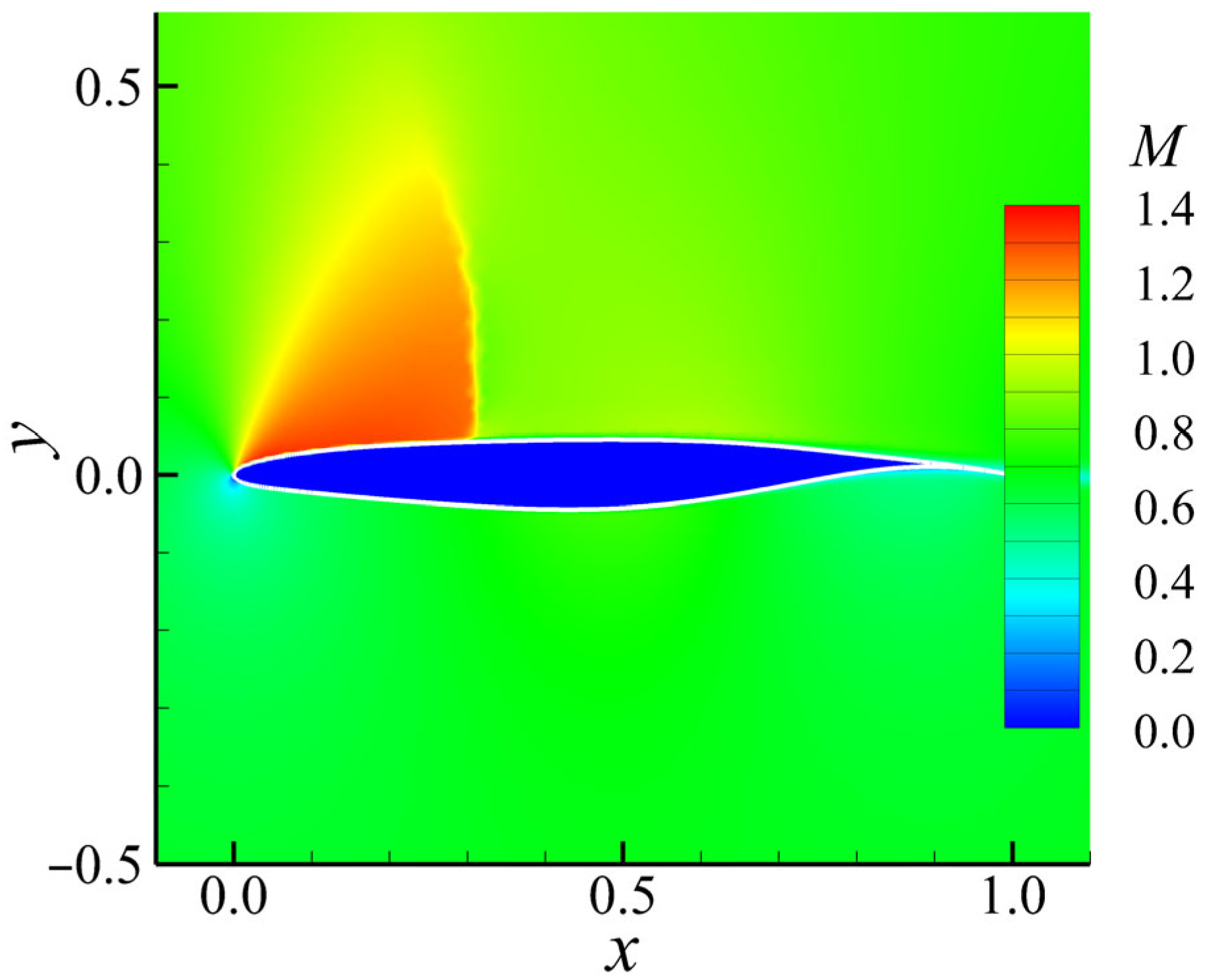
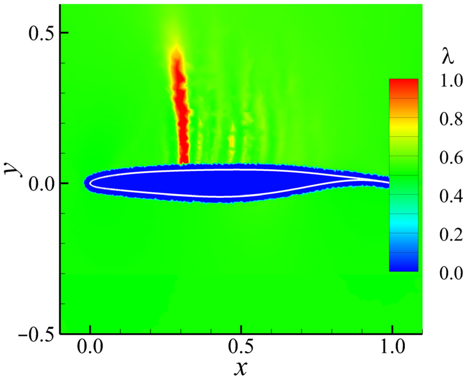
Figure 7 illustrates the ground-truth Mach-number field for a representative supercritical airfoil at a free-stream Mach number of $M_{\mathrm{\infty }}=0.71$ and an angle of attack of 2.75 degrees. Figure 8 shows the distribution of the pointwise weight $\lambda$ used to improve the prediction accuracy of key flow structures. The weight $\lambda$ is computed from the current model predictions, which may introduce occasional false identifications outside the shock region. In practice, these spurious detections have a negligible impact on the training process and do not degrade convergence.

Overall, Equation (9) is essentially a soft reweighting of the standard MSE loss. The shock wave and boundary layer identification functions are smooth, avoiding discontinuities that could destabilize training. The resulting weights are bounded and normalized, preventing over-dominance of localized regions. Therefore, the proposed loss acts as an adaptive importance-sampling mechanism rather than enforcing PDE residuals as in PINNs, which improves numerical robustness and reproducibility. The parameters in Equations (6)–(8) are determined empirically to provide sufficiently broad identification regions for shock waves and boundary layers. Because these functions only serve to reweight the loss, the training is not highly sensitive to their exact values, so that the relaxed parameter choices do not adversely affect convergence or accuracy.

3.3. Single-Resolution and Multi-Resolution Models

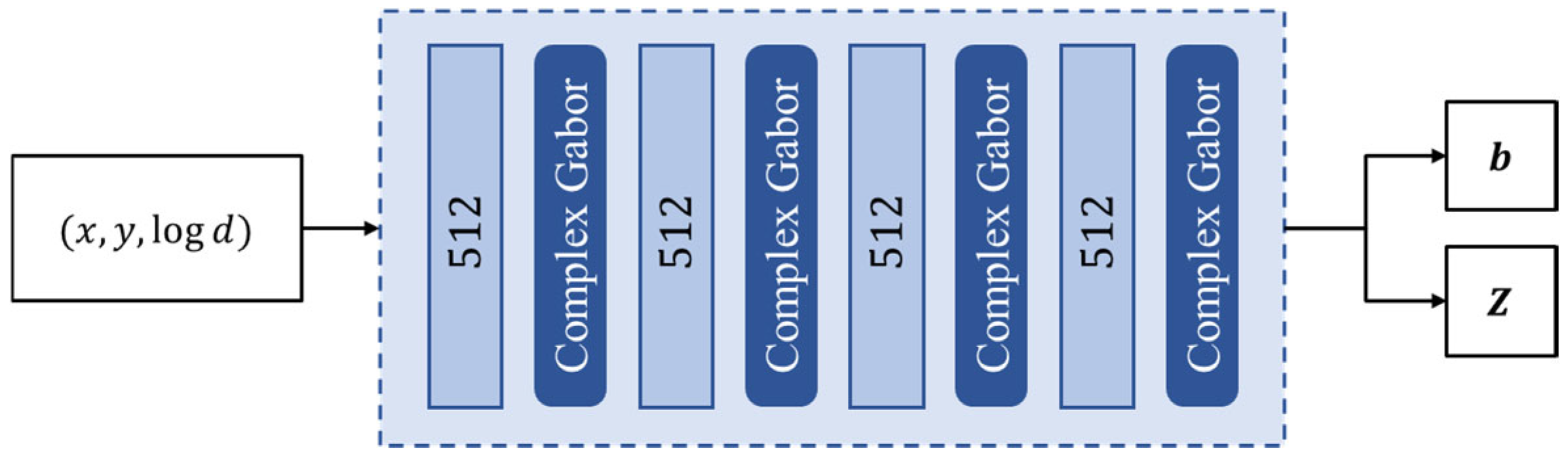
Two models are investigated in this study. Model 1 employs a single-resolution ShapeNet, whereas model 2 adopts a multi-resolution ShapeNet. Both models share the same HyperNet, which comprises four hidden layers with 512 neurons each and uses the ReLU activation function. The latent dimension is set to $n_l=512$. Figure 9 illustrates the architecture of the single-resolution ShapeNet, which uses a two-dimensional continuous complex Gabor wavelet $\psi$ as the activation function:

$$\psi \left(x;{\omega }_0,s_0\right)=e^{j{\omega }_{0}x}{e^{\left|s_{0}x\right|}}^2,$$

(10)

where $x$ is a complex number, $j$ is the imaginary unit, ${\omega }_0$ controls the frequency of the wavelet, and $s_0$ controls the spread (or width). It was first proposed in the multi-dimensional wavelet implicit representations (WIRE) [35]. In this study, ${\omega }_0$ and $s_0$ are both set to 30, and the detailed implementation of the complex Gabor wavelet can be found in [35]. In previous studies, the ${\omega }_0$-scaled sine activation function (Sinusoidal Representation Network, SIREN [21]) is usually used in INR-based mesh-agnostic models, especially for flow fields with high-frequency structures or discontinuities [36]. However, WIRE has higher representation capacity, achieves higher accuracy at a faster rate, and can be used to capture non-homogeneous high-frequency flow structures.

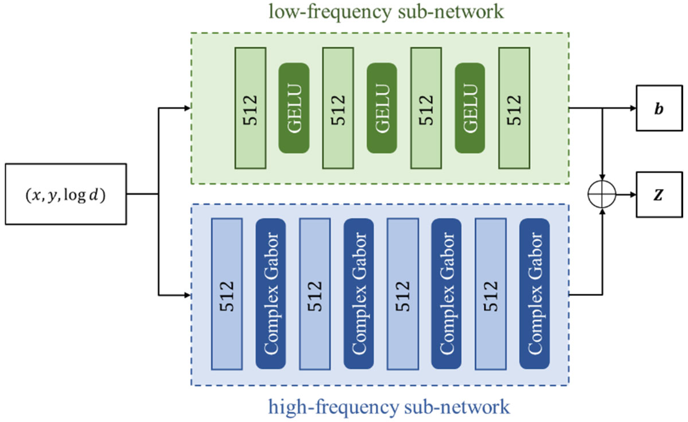
Meanwhile, a multi-resolution ShapeNet is introduced to better capture flow features across disparate spatial scales. As shown in Figure 10, ShapeNet is decomposed into two parallel subnetworks. Both subnetworks consist of four hidden layers with 512 neurons each. The high-frequency branch uses the complex Gabor function as its activation, while the low-frequency branch adopts the Gaussian Error Linear Unit (GELU) activation. GELU is a smooth, differentiable nonlinearity that is related to classic ELU and ReLU functions and often achieves better empirical performance [37]. In addition, its differentiability facilitates the computation of spatial gradients in the proposed mesh-agnostic framework. Accordingly, the multi-resolution model is expected to learn the mean flow (i.e., the bias $\mathbf{b}$) and large-scale structures using the low-frequency branch while capturing fine-scale features—such as shock waves and boundary layers—using the high-frequency branch.

3.4. Summary

Although the overall formulation is inspired by DeepONet-style operator learning, the proposed architecture is tailored to transonic flow prediction through geometry-aware inputs, multi-resolution implicit representations, and physics-guided training strategies, which are absent in standard DeepONet formulations. Compared with the previous work on mesh-agnostic implicit decoders for airfoil pressure prediction [28], the present study significantly extends both the modeling scope and the methodological design. Instead of predicting surface pressure distributions only, the proposed framework is developed for full-field prediction of two-dimensional transonic viscous flows, which involves substantially higher dimensionality and more complex flow physics. In addition, this work explicitly targets the accurate representation of shock waves and boundary layers by incorporating the distance-to-surface as a geometric input, introducing a multi-resolution implicit representation, and designing a physics-guided loss function to emphasize large-gradient regions. These extensions enable the implicit decoder to serve as a general-purpose, mesh-agnostic flow field predictor for transonic aerodynamic applications rather than a surface-based surrogate model.

4. Flow Field Prediction of Supercritical Airfoils

4.1. Influence of the Distribution of Training Data Points

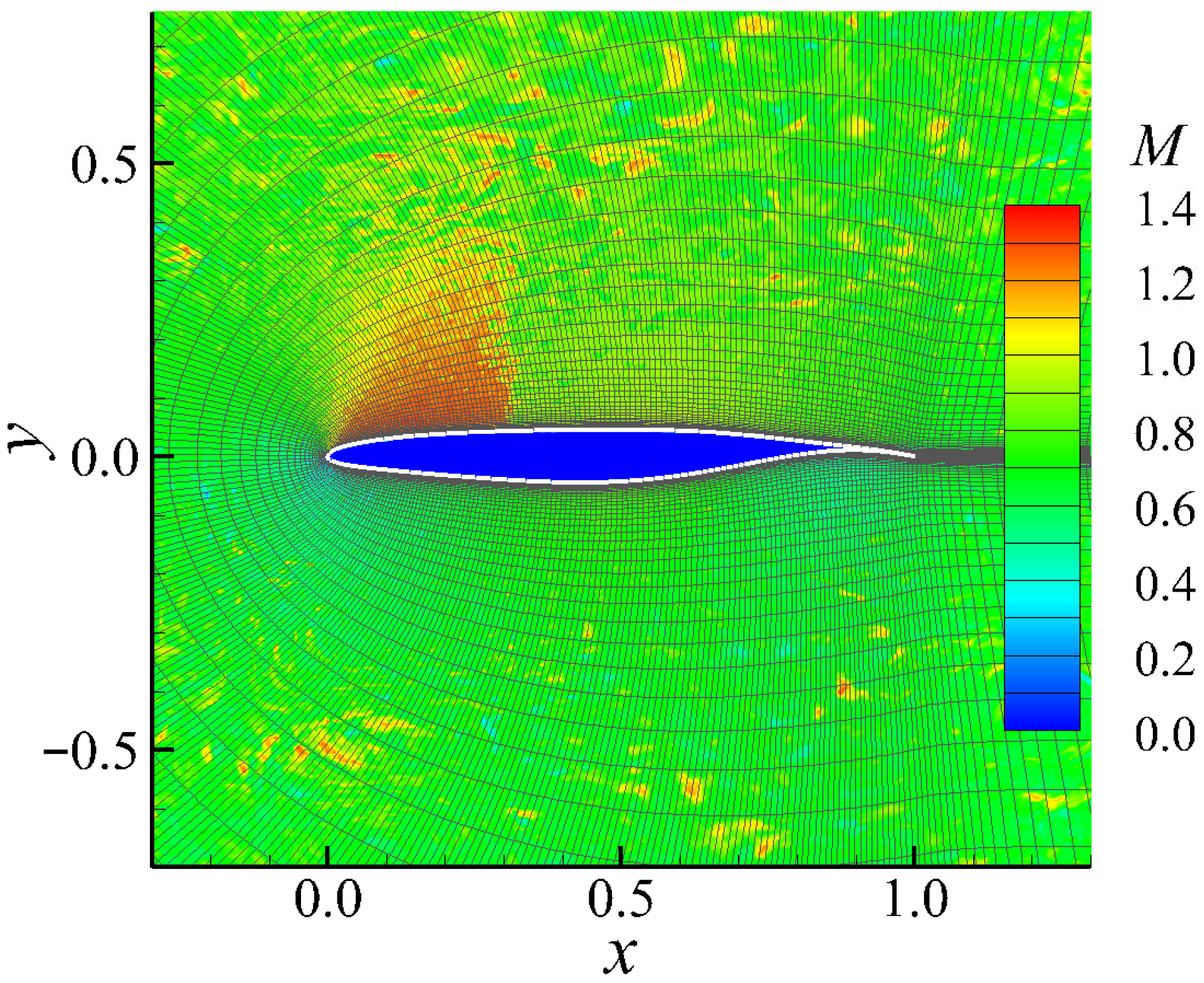
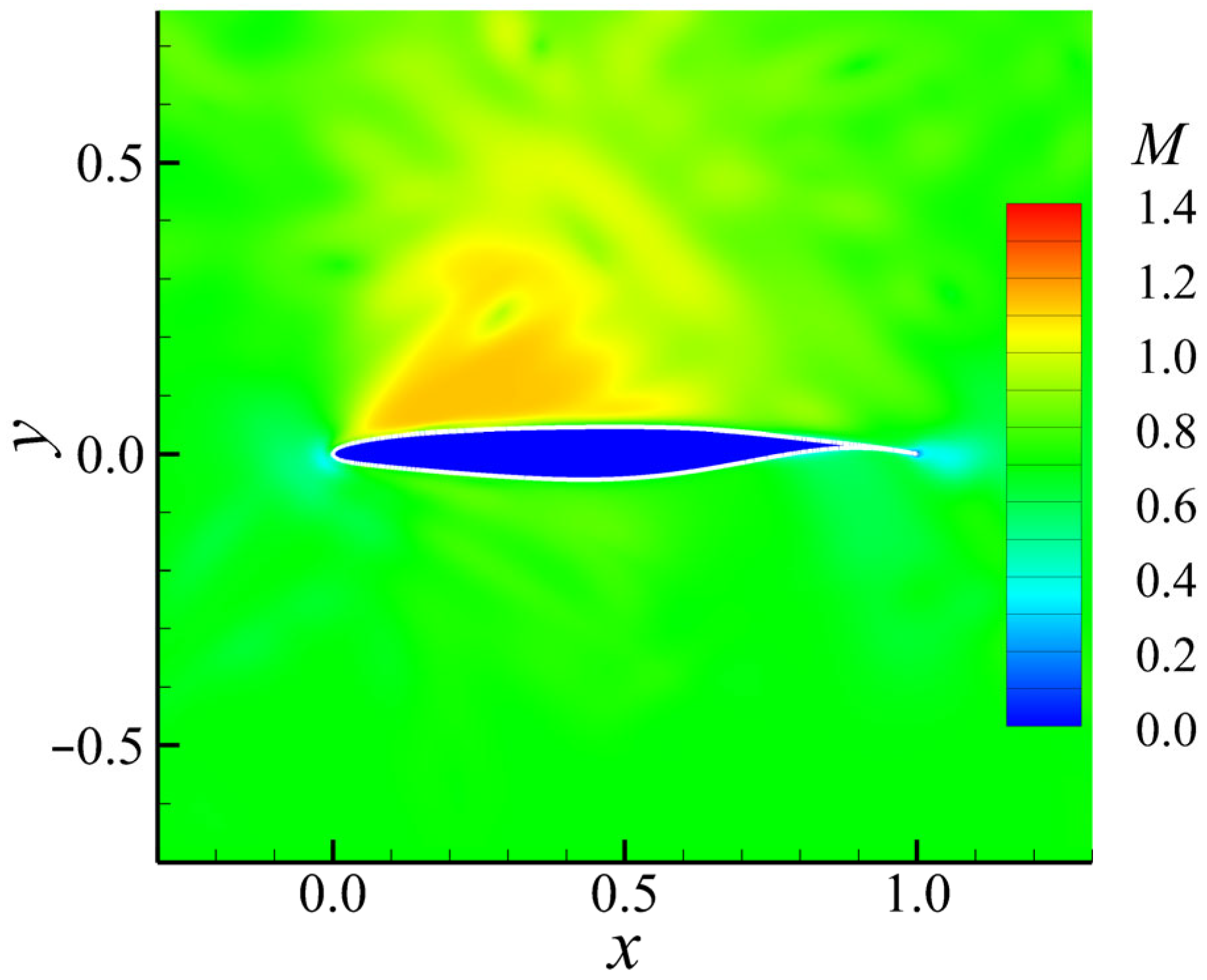
Mesh-agnostic models can generate predictions at arbitrary resolutions; however, this flexibility can also make training more challenging. As discussed in Section 2.2, training on flow field samples with a fixed grid point distribution may encourage overfitting. Figure 11 presents the Mach number prediction of a mesh-agnostic model trained using the original C–H grids shown in Figure 4a. The gray lines indicate the training grid, and the white curve denotes the airfoil surface. For visualization, the flow field is evaluated on a Cartesian grid over the domain $x\in [-0.5, 1.5]$ and $y\in [-1.0, 1.0]$, with 401 points in each direction. As shown in Figure 11, the model tends to overfit the training grid, leading to larger prediction errors in regions between grid lines. Therefore, all subsequent results are obtained by training on the randomly sampled points illustrated in Figure 4b.

4.2. Improving the Prediction Accuracy for Various Geometries

When predicting flow fields for different airfoils, the solution can vary substantially, particularly in the boundary layer region. At the same spatial location $\left(x,y\right)$, the corresponding near-wall coordinate $y^{+}$ may differ across airfoils, leading to significant variations in the local flow variables. Moreover, a point that lies in the fluid domain for one airfoil may fall inside the solid body for another, thereby yielding invalid values. As discussed in Section 3.1, these issues present a major challenge for mesh-agnostic models and can lead to underfitting when the geometry is not sufficiently encoded.

Figure 12 shows the Mach number prediction of the proposed model when only $(x,y)$ are used as inputs to ShapeNet. Compared with the ground-truth field in Figure 7, the prediction is clearly underfitted. Therefore, the logarithm of the distance to the surface, $\log d$, is included as an additional model input, as introduced in Section 3.1.

4.3. Improving the Prediction Accuracy for Flow Structures

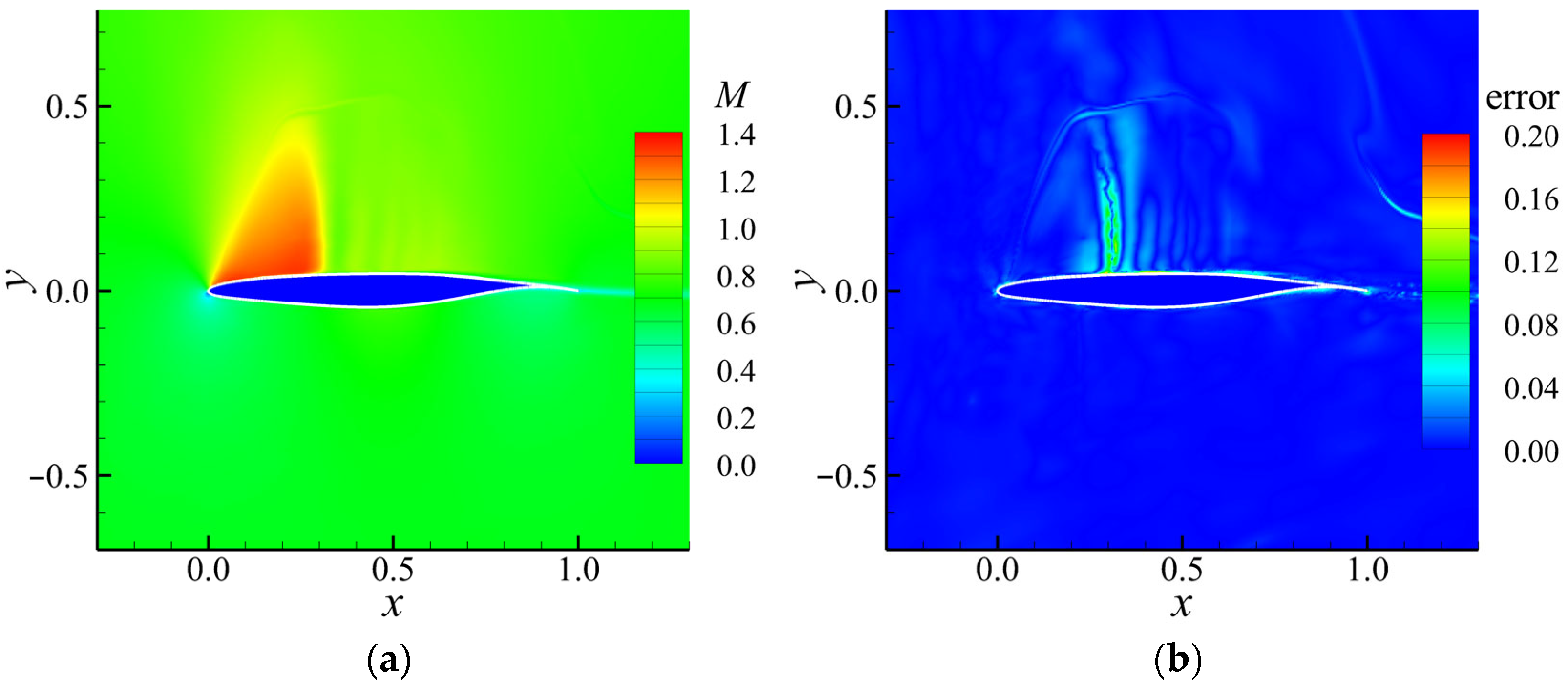
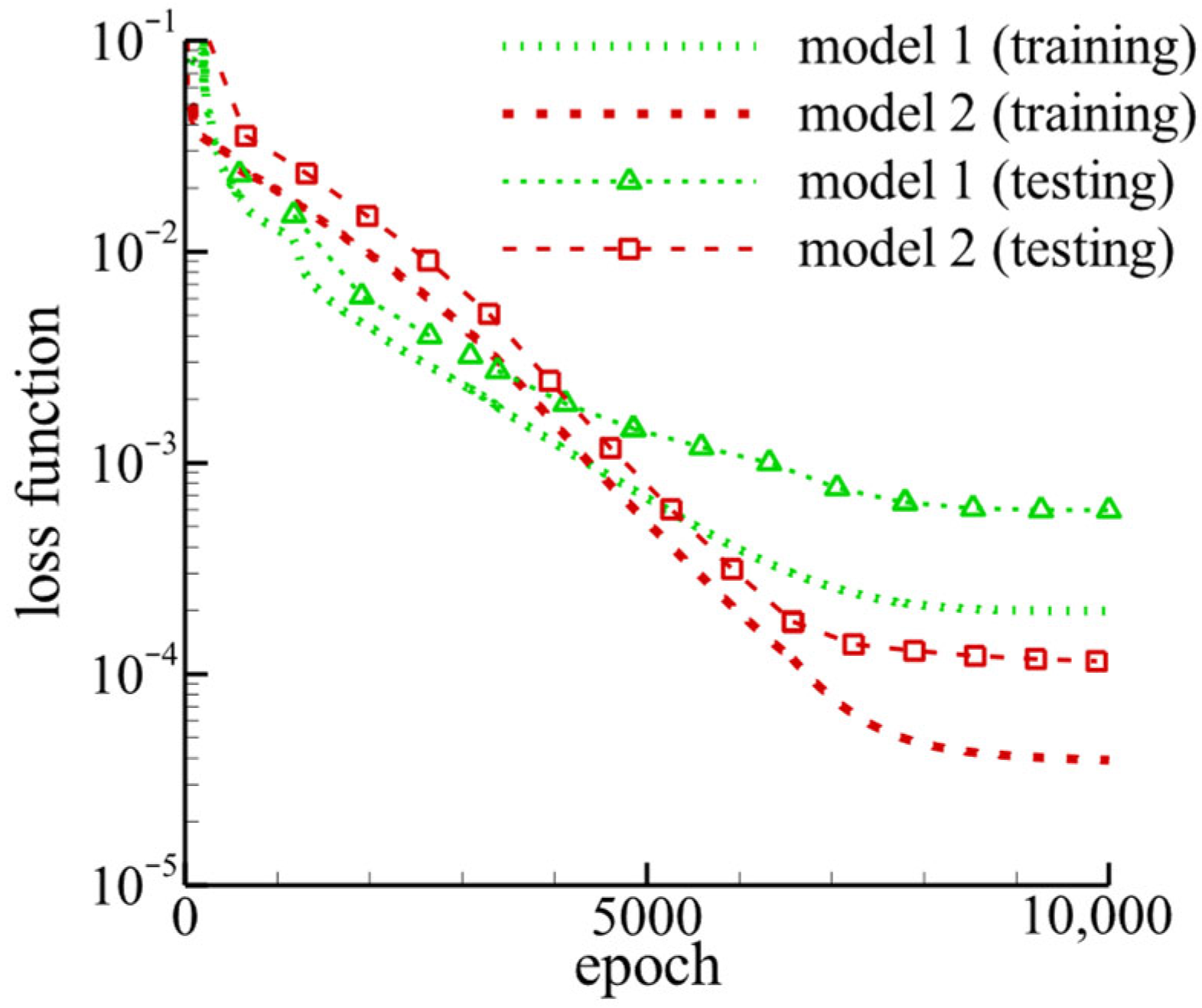
To examine the effects of the multi-resolution ShapeNet and the physics-guided loss, two models are compared in this section: (1) model 1, a single-resolution model trained without the physics-guided loss, in which ShapeNet consists only of the high-frequency branch with the complex Gabor activation (Figure 10); and (2) model 2, a multi-resolution model using the full ShapeNet in Figure 10 together with the physics-guided loss function in Equation (9). Both models are trained and evaluated using the training and testing sets described in Section 2.1. Model 1 is trained by minimizing the unweighted MSE loss, i.e., Equation (5), whereas model 2 is trained by minimizing the physics-guided loss, i.e., Equation (9). For clarity, the training history of the unweighted MSE loss is shown in Figure 13. In Figure 13, dashed lines indicate the average prediction error on the training set, and dashed lines with markers indicate the average prediction error on the testing set. As shown, model 2 achieves a lower overall prediction error.

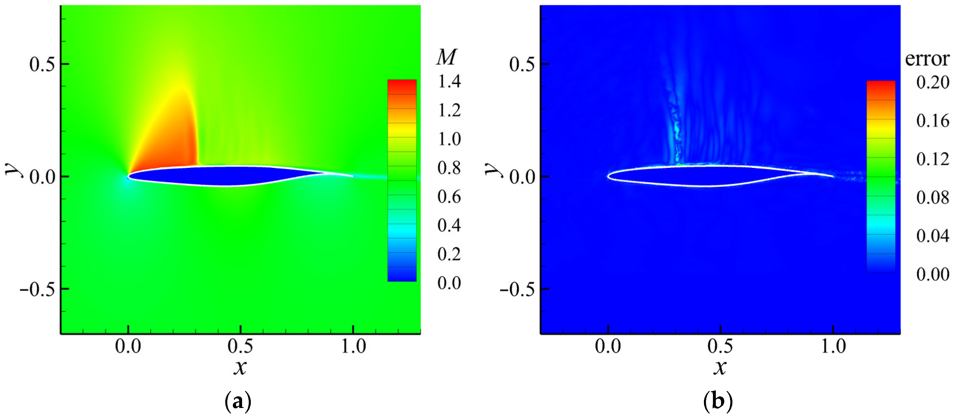
Figure 14 presents the predicted Mach number field of model 1 and the corresponding absolute error distribution, while Figure 15 shows the results of model 2. For both models, predictions are evaluated on a Cartesian grid over the domain $x\in [-0.5, 1.5]$ and $y\in [-1.0, 1.0]$, with 401 points in each direction. The airfoil surface is indicated by the white curve. The absolute error is computed as the difference between the predicted values and the reference values interpolated from the ground-truth flow field using the dual-linear Coons transfinite interpolation in Equation (3).

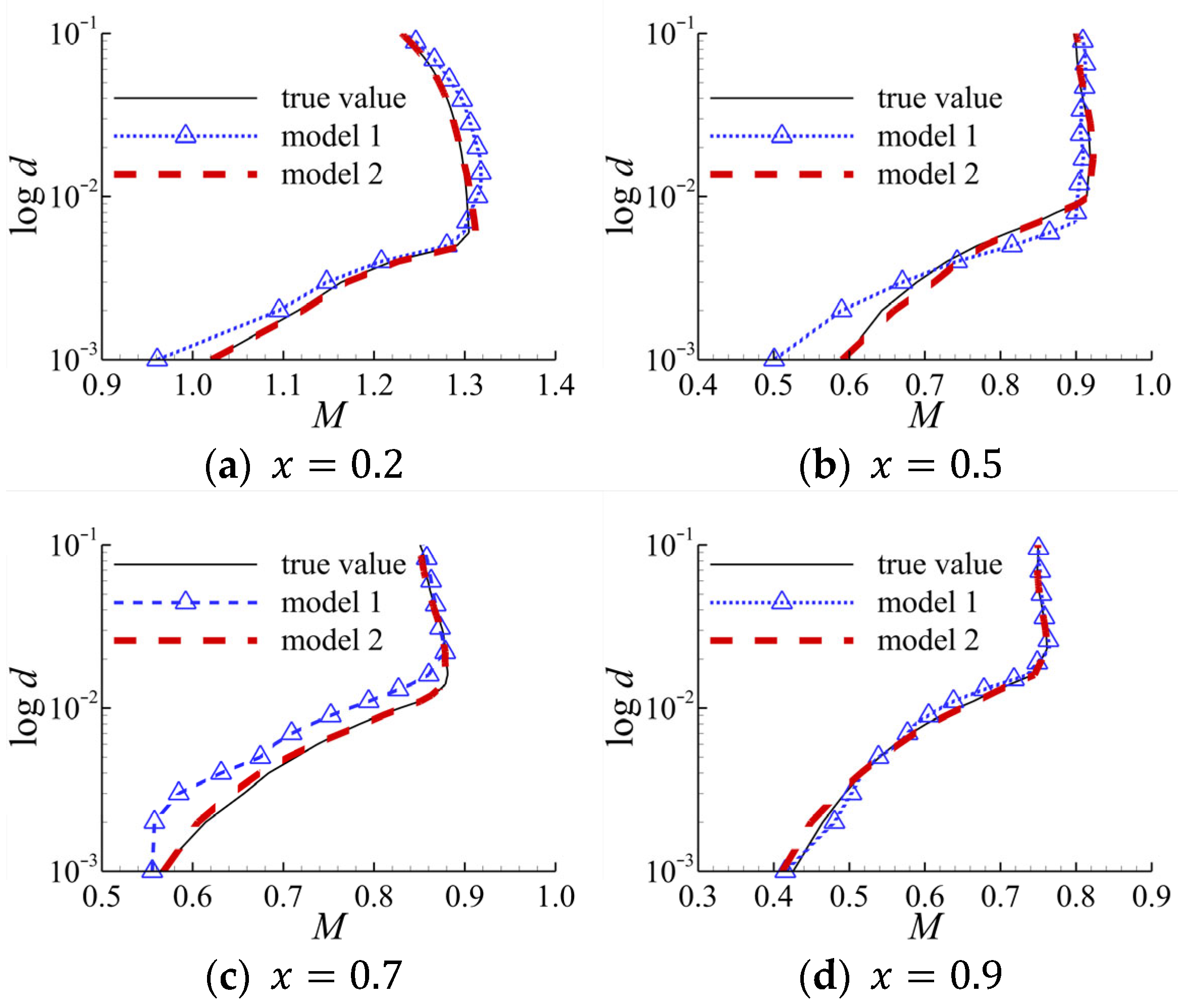
Figure 16 further compares the two models within the boundary layer on the upper surface. Four chordwise locations are selected, namely $x=0.2$, $0.5$, $0.7$, $0.9$. At each location, the Mach number is sampled along the wall-normal direction over $d\in [0, 0.1]$ using 100 evenly spaced points. The corresponding reference values are obtained by interpolation from the ground-truth solution. The results demonstrate that combining the multi-resolution ShapeNet with the physics-guided loss significantly improves the prediction accuracy of the proposed mesh-agnostic model.

4.4. Model Validation on Test Airfoils

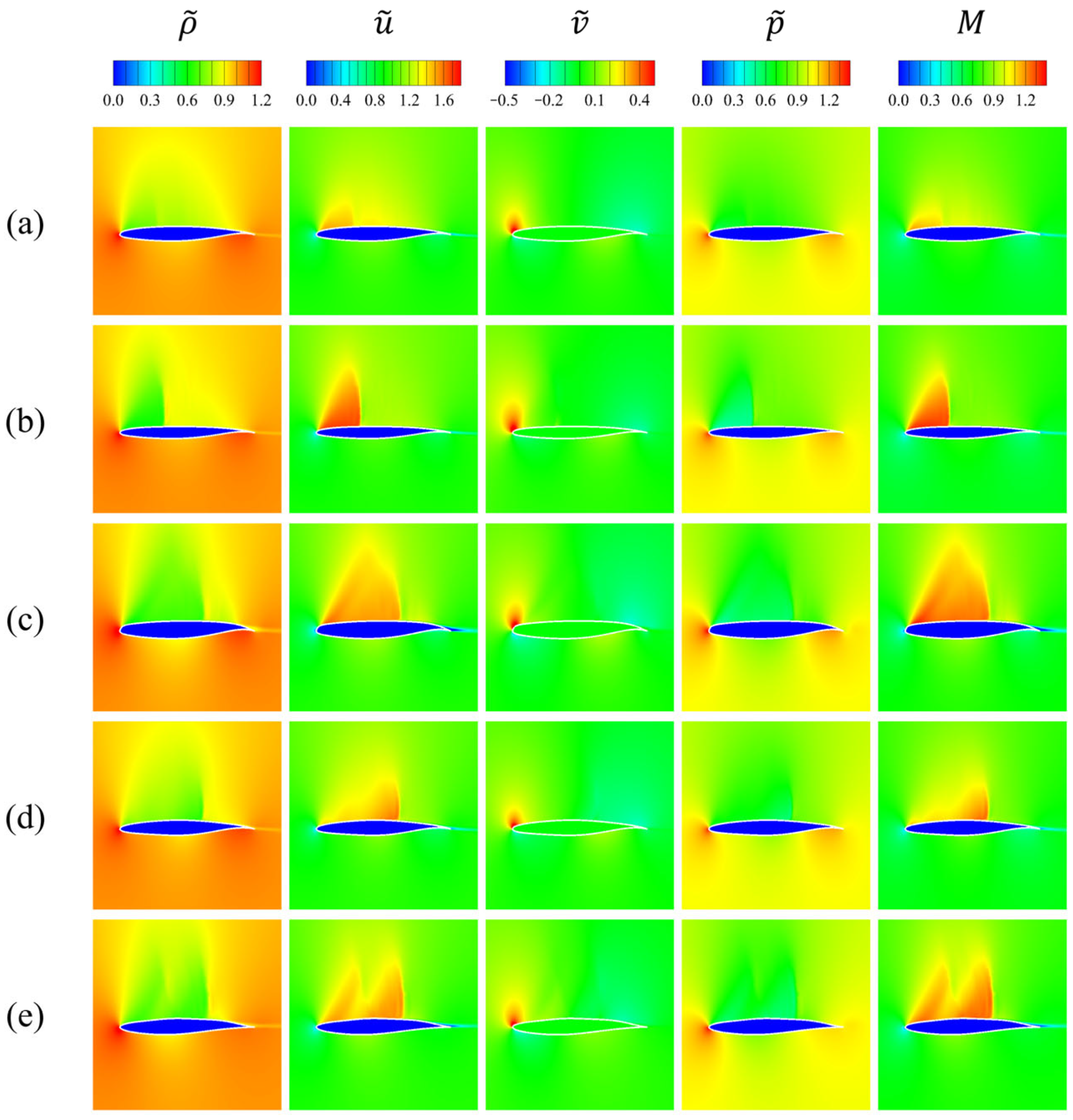
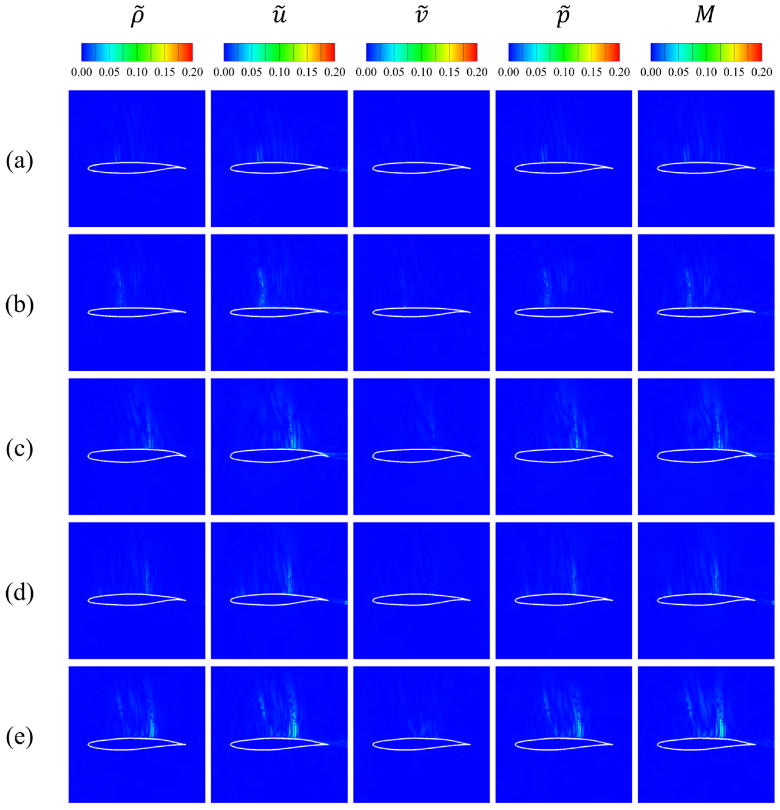
The proposed model is validated on the testing set, and five representative airfoils are selected for detailed comparison (

Table 1. Typical airfoil samples in the test set.

Sub-Figure	${\mathit{M}}_{\mathit{\infty }}$	$\mathit{A}\mathit{o}\mathit{A}$	${\mathit{C}}_{\mathbf{L}}$	${\mathit{C}}_{\mathbf{m}}$	${\mathit{t}}_{\mathbf{m}\mathbf{a}\mathbf{x}}$
(a)	0.710	1.313	0.780	−0.142	0.110
(b)	0.710	2.592	0.900	−0.108	0.090
(c)	0.750	1.245	0.840	−0.166	0.130
(d)	0.723	1.394	0.809	−0.157	0.114
(e)	0.750	2.699	0.760	−0.103	0.120

). Figure 17 presents the predicted non-dimensional flow field variables, while Figure 18 shows the corresponding absolute prediction errors. The error maps indicate that the discrepancies are primarily concentrated in the shock wave region, with a maximum local absolute error of approximately 5%.

The flow variables are non-dimensionalized following the convention used in CFL3D:

$$\tilde{\rho }=\rho /{\rho }_{\infty }, \tilde{u}=u/a_{\infty }, \tilde{v}=v/a_{\infty }, \tilde{p}=p/p_{\infty }.$$

(11)

The five test airfoils span a range of free-stream Mach numbers, angles of attack, lift coefficients, maximum relative thicknesses, and associated flow structures. Airfoil (a) exhibits a very weak shock, airfoils (b)–(d) feature shocks with different locations and strengths, and airfoil (e) contains a double-shock structure.

All experiments were conducted on a workstation equipped with a single NVIDIA A10 GPU (24 GB memory). Owing to the large-scale training dataset, where each spatial point is treated as an independent training instance, the training stage is the main computational bottleneck. Training one model requires approximately 20 h. However, the inference stage is highly efficient, i.e., predicting a complete flow field for a given airfoil and free-stream condition takes less than 1 s. This low inference cost makes the proposed mesh-agnostic model well suited for fast aerodynamic analysis and machine-learning-assisted optimization workflows.

Overall, the results demonstrate that the proposed model provides accurate predictions across all these transonic flow fields. However, it also should be noted that the generalization capability discussed in this work refers to interpolation within a broad but well-defined parametric space rather than unrestricted extrapolation. The training and testing datasets cover a wide range of supercritical airfoil geometries, free-stream Mach numbers, and angles of attack that are representative of transonic civil aircraft applications. The results demonstrate that the proposed model can accurately predict flow fields for unseen airfoil geometries and flow conditions within this distribution, including cases with different shock locations and strengths.

5. Conclusions

In recent years, machine learning has been extensively investigated for aerodynamic design. However, its application to three-dimensional aircraft configurations remains limited, mainly due to the high computational cost of data generation and the challenges associated with data formatting. Mesh-agnostic models offer the flexibility to leverage data from meshes with varying topologies and resolutions, which is particularly attractive for learning two- and three-dimensional flows over complex geometries. To date, most mesh-agnostic approaches have been demonstrated on relatively simple problems, such as turbulent channel flows and subsonic flows around airfoils. In this study, we develop a mesh-agnostic implicit decoder based on DeepONet for transonic viscous flows around various supercritical airfoils under different free-stream conditions. The main conclusions are summarized as follows.

• The implicit decoder comprises two subnetworks: ShapeNet and HyperNet. ShapeNet provides a mesh-agnostic implicit neural representation that outputs spatial bases of the transonic flow field. HyperNet predicts the corresponding weights conditioned on the input parameters, such that the flow field is expressed as a linear combination of these bases. Owing to this formulation, the implicit decoder can serve as a drop-in replacement for conventional decoders in standard machine learning pipelines.
• The distance to the airfoil surface, $d$, is introduced as an auxiliary geometric input to ShapeNet together with the point coordinates $(x,y)$, enabling the model to better resolve boundary layer variations across different geometries. To mitigate overfitting associated with the highly non-uniform point distribution in the flow field, the logarithm of the distance, $\log d$, is used. The results show that incorporating $\log d$ substantially improves prediction accuracy.
• Accurately capturing transonic flow structures poses a multi-resolution learning challenge: sampling density is much higher in the boundary layer, while shock waves feature sharp gradients that require enhanced effective resolution. To address this, a multi-resolution ShapeNet is proposed. A low-frequency branch with the smoother GELU activation is employed to learn the mean flow and large-scale features, whereas a high-frequency branch using complex Gabor activations captures fine-scale structures. In addition, a physics-guided loss function is introduced to further improve shock wave prediction accuracy.

The results demonstrate that the proposed mesh-agnostic model can accurately predict transonic flow fields for a wide range of airfoil geometries under varying free-stream conditions. The model captures both shock wave structures and boundary layer velocity profiles with good fidelity. These findings suggest that the proposed approach provides a promising foundation for extending machine-learning-based flow prediction to more complex geometries and ultimately to three-dimensional configurations.

The present study demonstrates reliable interpolation performance within the trained design space of transonic supercritical airfoils. Extending the proposed approach to other flow regimes and three-dimensional configurations remains a topic for future investigation. The Reynolds number may be incorporated into the HyperNet conditioning vector (e.g., using a logarithmic form), and future datasets could include sampled Reynolds numbers to enable learning of Reynolds-dependent flow effects. In addition, future work will explore the integration of the proposed model into inverse-design frameworks and further assess its performance under a broader range of geometric variations.

References

1. Li, J.; Du, X.; Martins, J.R.R.A. Machine Learning in Aerodynamic Shape Optimization. Prog. Aerosp. Sci. 2022, 134, 100849. [Google Scholar] [CrossRef]
2. Du, X.; He, P.; Martins, J.R.R.A. Rapid Airfoil Design Optimization via Neural Networks-Based Parameterization and Surrogate Modeling. Aerosp. Sci. Technol. 2021, 113, 106701. [Google Scholar] [CrossRef]
3. Li, J.; Zhang, M.; Martins, J.R.R.A.; Shu, C. Efficient Aerodynamic Shape Optimization with Deep-Learning-Based Geometric Filtering. AIAA J. 2020, 58, 4243–4259. [Google Scholar] [CrossRef]
4. Brunton, S.L.; Noack, B.R.; Koumoutsakos, P. Machine Learning for Fluid Mechanics. Annu. Rev. Fluid Mech. 2019, 52, 477–508. [Google Scholar] [CrossRef]
5. Li, R.; Deng, K.; Zhang, Y.; Chen, H. Pressure Distribution Guided Supercritical Wing Optimization. Chin. J. Aeronaut. 2018, 31, 1842–1854. [Google Scholar] [CrossRef]
6. Wu, M.-Y.; Wu, Y.; Yuan, X.-Y.; Chen, Z.-H.; Wu, W.-T.; Aubry, N. Fast Prediction of Flow Field around Airfoils Based on Deep Convolutional Neural Network. Appl. Sci. 2022, 12, 12075. [Google Scholar] [CrossRef]
7. Sekar, V.; Jiang, Q.; Shu, C.; Khoo, B.C. Fast Flow Field Prediction over Airfoils Using Deep Learning Approach. Phys. Fluids 2019, 31, 057103. [Google Scholar] [CrossRef]
8. Wang, J.; He, C.; Li, R.; Chen, H.; Zhai, C.; Zhang, M. Flow Field Prediction of Supercritical Airfoils via Variational Autoencoder Based Deep Learning Framework. Phys. Fluids 2021, 33, 086108. [Google Scholar] [CrossRef]
9. Yang, Y.; Li, R.; Zhang, Y.; Chen, H. Flowfield Prediction of Airfoil Off-Design Conditions Based on a Modified Variational Autoencoder. AIAA J. 2022, 60, 5805–5820. [Google Scholar] [CrossRef]
10. Chen, D.; Gao, X.; Xu, C.; Chen, S.; Fang, J.; Wang, Z.; Wang, Z. FlowGAN: A Conditional Generative Adversarial Network for Flow Prediction in Various Conditions. In Proceedings of the 2020 IEEE 32nd International Conference on Tools with Artificial Intelligence (ICTAI), Baltimore, MD, USA, 9–11 November 2020. [Google Scholar] [CrossRef]
11. Wu, H.; Liu, X.; An, W.; Lyu, H. A Generative Deep Learning Framework for Airfoil Flow Field Prediction with Sparse Data. Chin. J. Aeronaut. 2022, 35, 470–484. [Google Scholar] [CrossRef]
12. Gupta, R.; Jaiman, R. Three-Dimensional Deep Learning-Based Reduced Order Model for Unsteady Flow Dynamics with Variable Reynolds Number. Phys. Fluids 2022, 34, 033612. [Google Scholar] [CrossRef]
13. Sabater, C.; Stürmer, P.; Bekemeyer, P. Fast Predictions of Aircraft Aerodynamics Using Deep-Learning Techniques. AIAA J. 2022, 60, 5249–5261. [Google Scholar] [CrossRef]
14. Immordino, G.; Da Ronch, A.; Righi, M. Deep–Learning Framework for Aircraft Aerodynamics Prediction. In Proceedings of the AIAA AVIATION 2023 Forum, San Diego, CA, USA, 12–16 June 2023. [Google Scholar] [CrossRef]
15. Hu, J.; Zhang, W. Flow Field Modeling of Airfoil Based on Convolutional Neural Networks from Transform Domain Perspective. Aerosp. Sci. Technol. 2023, 136, 108198. [Google Scholar] [CrossRef]
16. Li, R.; Zhang, Y.; Chen, H. Transfer Learning from Two-Dimensional Supercritical Airfoils to Three-Dimensional Transonic Swept Wings. Chin. J. Aeronaut. 2023, 36, 96–110. [Google Scholar] [CrossRef]
17. Chen, J.; Zhao, J.; Xiao, W.; Lv, L.; Zhao, W.; Wu, X. A Multi-Fidelity Uncertainty Propagation Model for Multi-Dimensional Correlated Flow Field Responses. Aerospace 2024, 11, 263. [Google Scholar] [CrossRef]
18. Li, J.; Li, Y.; Liu, T.; Zhang, D.; Xie, Y. Multi-Fidelity Graph Neural Network for Flow Field Data Fusion of Turbomachinery. Energy 2023, 285, 129405. [Google Scholar] [CrossRef]
19. Goodfellow, I.; Bengio, Y.; Courville, A. Deep Learning; MIT Press: Cambridge, MA, USA, 2016; p. 413. [Google Scholar]
20. Bhatnagar, S.; Afshar, Y.; Pan, S.; Duraisamy, K.; Kaushik, S. Prediction of Aerodynamic Flow Fields Using Convolutional Neural Networks. Comput. Mech. 2019, 64, 525–545. [Google Scholar] [CrossRef]
21. Sitzmann, V.; Martel, J.N.P.; Bergman, A.W.; Lindell, D.B.; Wetzstein, G. Implicit Neural Representations with Periodic Activation Functions. In Proceedings of the Advances in Neural Information Processing Systems (NeurIPS), Online, 6–12 December 2020. [Google Scholar] [CrossRef]
22. Ogoke, F.; Meidani, K.; Hashemi, A.; Farimani, A.B. Graph Convolutional Networks Applied to Unstructured Flow Field Data. Mach. Learn. Sci. Technol. 2021, 2, 045020. [Google Scholar] [CrossRef]
23. Shen, Y.; Huang, W.; Wang, Z.; Xu, D.; Liu, C.-Y. A Deep Learning Framework for Aerodynamic Pressure Prediction on General Three-Dimensional Configurations. Phys. Fluids 2023, 35, 107111. [Google Scholar] [CrossRef]
24. Cai, S.; Mao, Z.; Wang, Z.; Yin, M.; Karniadakis, G.E. Physics-Informed Neural Networks (PINNs) for Fluid Mechanics: A Review. Acta Mech. Sin. 2021, 37, 1727–1738. [Google Scholar] [CrossRef]
25. Lu, L.; Jin, P.; Karniadakis, G.E. DeepONet: Learning Nonlinear Operators for Identifying Differential Equations Based on the Universal Approximation Theorem of Operators. Nat. Mach. Intell. 2021, 3, 218–229. [Google Scholar] [CrossRef]
26. Pan, S.; Brunton, S.L.; Kutz, J.N. Neural Implicit Flow: A Mesh-Agnostic Dimensionality Reduction Paradigm of Spatio-Temporal Data. arXiv 2023, arXiv:2204.03216. [Google Scholar] [CrossRef]
27. Shukla, K.; Oommen, V.; Peyvan, A.; Penwarden, M.; Plewacki, N.; Bravo, L.; Ghoshal, A.; Kirby, R.M.; Karniadakis, G.E. Deep Neural Operators as Accurate Surrogates for Shape Optimization. Eng. Appl. Artif. Intell. 2024, 129, 107615. [Google Scholar] [CrossRef]
28. Li, R.; Zhang, Y.; Chen, H. Mesh-Agnostic Decoders for Supercritical Airfoil Prediction and Inverse Design. AIAA J. 2024, 62, 1–17. [Google Scholar] [CrossRef]
29. Ha, D.; Dai, A.; Le, Q.V. HyperNetworks. arXiv 2016, arXiv:1609.09106. [Google Scholar] [CrossRef]
30. Kulfan, B.M. Universal Parametric Geometry Representation Method. J. Aircr. 2008, 45, 142–158. [Google Scholar] [CrossRef]
31. NASA Langley Research Center, NASA Technology Transfer Program. Computational Fluids Laboratory 3-Dimensional (CFL3D Version 6.7). Available online: https://nasa.github.io/CFL3D/Cfl3dv6/cfl3dv6_home.html (accessed on 24 December 2025).
32. Li, R.; Zhang, Y.; Chen, H. Knowledge Discovery with Computational Fluid Dynamics: Supercritical Airfoil Database and Drag Divergence Prediction. Phys. Fluids 2023, 35, 016113. [Google Scholar] [CrossRef]
33. Délery, J.; Marvin, G.; Reshotko, E. Shock-Wave Boundary Layer Interactions; AGARD-AG-280; Advisory Group for Aerospace Research and Development (AGARD): Neuilly-sur-Seine, France, 1986. [Google Scholar]
34. Kingma, D.P.; Ba, J. Adam: A Method for Stochastic Optimization. arXiv 2014, arXiv:1412.6980. [Google Scholar] [CrossRef]
35. Saragadam, V.; LeJeune, D.; Tan, J.; Balakrishnan, G.; Veeraraghavan, A.; Baraniuk, R.G. WIRE: Wavelet Implicit Neural Representations. In Proceedings of the IEEE/CVF Conference on Computer Vision and Pattern Recognition (CVPR), Vancouver, BC, Canada, 17–24 June 2023; pp. 18507–18516. [Google Scholar] [CrossRef]
36. Rahaman, N.; Baratin, A.; Arpit, D.; Draxler, F.; Lin, M. On the Spectral Bias of Neural Networks. arXiv 2019, arXiv:1806.08734. [Google Scholar] [CrossRef]
37. Hendrycks, D.; Gimpel, K. Gaussian Error Linear Units (GELUs). arXiv 2016, arXiv:1606.08415. [Google Scholar] [CrossRef]
Figure 1. CFD validation and grid [32]. (a) Grid convergence study of C p . (b) Medium grid.
Aerospace 13 00117 g001
Figure 2. Classic supercritical airfoils [32].
Aerospace 13 00117 g002
Figure 3. Sample distributions in the parametric spaces [28].
Aerospace 13 00117 g003
Figure 4. The original C–H-type grid and the data points for training. (a) C–H-type grid. (b) Randomly sampled data points.
Aerospace 13 00117 g004
Figure 5. Distribution of data points based on different descriptions of distance to airfoil surface. (a) Distance to surface ( d ). (b) Logarithm of the distance to surface ( log d ).
Aerospace 13 00117 g005
Figure 6. Architecture of the mesh-agnostic model for flow field prediction.
Aerospace 13 00117 g006
Figure 7. Ground-truth Mach number field.
Aerospace 13 00117 g007
Figure 8. Distribution of the data point weight for capturing flow structures.
Aerospace 13 00117 g008
Figure 9. Architecture of the single-resolution ShapeNet (model 1).
Aerospace 13 00117 g009
Figure 10. Architecture of the multi-resolution ShapeNet (model 2).
Aerospace 13 00117 g010
Figure 11. Overfitting of flow field data on the uniform grids.
Aerospace 13 00117 g011
Figure 12. Mach number field prediction without d as model input.
Aerospace 13 00117 g012
Figure 13. MSE loss function history of the two models.
Aerospace 13 00117 g013
Figure 14. Prediction results of the single-resolution model (model 1). (a) Prediction of the Mach number field. (b) Distribution of the absolute error.
Aerospace 13 00117 g014
Figure 15. Prediction results of the multi-resolution model with physical loss functions (model 2). (a) Prediction of the Mach number field. (b) Distribution of the absolute error.
Aerospace 13 00117 g015
Figure 16. Mach number distribution in the boundary layer of the airfoil upper surface.
Aerospace 13 00117 g016
Figure 17. Prediction results of the mesh-agnostic model (model 2) on test samples.
Aerospace 13 00117 g017
Figure 18. Absolute prediction error of the mesh-agnostic model (model 2) on test samples.
Aerospace 13 00117 g018