Robust Approximate Optimal Trajectory Tracking Control for Quadrotors

Abstract

This paper uses the adaptive dynamic programming (ADP) method to achieve optimal trajectory tracking control for quadrotors. Relying on an established mathematical model of a quadrotor, the approximate optimal trajectory tracking control, which consists of the steady-state control input and the approximate optimal feedback control input, is designed for a nominal system. Considering the compound disturbances in position and attitude dynamic models, disturbance observers are introduced. The estimated values are used to design robust compensation inputs to suppress the effect of the compound disturbances for good trajectory tracking performance. Theoretically, the Lyapunov theorem demonstrates the stability of a closed-loop system. The robustness and effectiveness of the proposed controller are confirmed by the simulation results.

1. Introduction

The miniaturization and reduction in cost of the relevant control components in aircraft, as well as the development and progress of computer and sensing and measurement technologies, have improved the stability of flight control systems and greatly facilitated the development of quadrotors [1]. The high operability, strong mobility and flexibility of quadrotors allow them to meet the specific needs of many projects, generally used in military, industrial and other fields [2,3]. A quadrotor system is multivariable, nonlinear and strongly coupled, and quadrotors will also be disturbed by the surrounding environment during flight [4]. These factors can affect the accuracy of quadrotor control systems. The requirements for high-accuracy and robust flight control in the design of controllers for quadrotors are stringent, and the design of a core control algorithm is a prerequisite for quadrotors to achieve a stable and high-precision flight performance. Therefore, the research and development of controllers for quadrotor systems is of great significance.

At present, it is no longer a problem to ensure the uniformity of quadrotors through control algorithms. Many controllers for quadrotors have been designed and are already in application [5]. Since the dynamics of quadrotors can be linearized around the equilibrium point, traditional linear control methods are used for a designed controller [6]. On this basis, linear techniques are employed in the flight control of quadrotors, such as linear quadratic regulator (LQR) control [7]. However, quadrotors need to be controlled away from the equilibrium point to accomplish complex control tasks and withstand external disturbances. As a result, a technique has been devised that is regarded as a robust feedback linearization method that uses extended state observers to estimate the nonlinear state feedback term online, containing aerodynamic forces, moments and unknown disturbances, and obtains the desired closed-loop dynamics via pole assignment [8]. Moreover, several robust controllers relying on nonlinear techniques have been proposed, such as sliding mode control [9], adaptive control [10], backstepping-based control [11] and robust control [12]. These control methods ensure the stability and robustness of nonlinear systems and have generally been used for the tracking control of these systems, but their optimal properties have not been considered. Therefore, the concept of optimization has been introduced into control design.

To derive the optimal control policy for the infinite horizon optimal control problem, solving the Hamilton–Jacobi–Bellman (HJB) equation or the Hamilton–Jacobi–Isaacs (HJI) equation for the $H_{\infty }$ optimal control problem considering uncertainties is essential. Nevertheless, it is difficult to mathematically derive the corresponding analytical solutions in most cases. Neural networks are an optional method to overcome this problem [13,14,15]. The approximation property of neural networks makes it possible to find approximate solutions to partial differential equations. The convergence of neural networks can be ensured by penalizing them to ensure they satisfy the given partial differential equations. The ADP method is the combination of reinforcement learning, dynamic programming and neural network adaptive methods to derive approximate solutions of the HJB/HJI equations using function approximate structures to address nonlinear optimal control problems [16,17]. The ADP method is used for control design with suitable performance index functions to derive the desired dynamic performance and stabilize a nominal system with uncertainties. However, most nonlinear optimal control methods using the ADP method are aimed at nominal systems or uncertain systems satisfying specific conditions [18,19,20], while the immunity to disturbances is still weak for such systems with external time-varying disturbances independent of the state, and the control effect under stronger disturbances is not ideal. The ADP method has been used in the design of controllers for quadrotors and efforts have been made to improve the robustness, but the designed controllers are more geared towards linear systems and design uncertainty is a unique problem [21,22]. Quadrotors will often experience various external effects in flight, requiring strong adaptive and anti-disturbance capabilities in flight control. The disturbance observer technique achieves disturbance suppression of the target utilizing feedback regulation [23], which can attenuate compound disturbances containing external disturbances and model uncertainties, thus improving the system robustness. A disturbance observer can accurately estimate compound disturbances in a system, which greatly reduces the conservatism of the control. In addition, since a disturbance observer can usually be designed independently of the controller, this ensures that the method can be easily combined with other advanced control methods and more flexible in its application. There are experiments suggesting that the introduction of a disturbance observer significantly improves performance, which is a good reference for methods for quadrotors to overcome disturbances [24].

Considering the above analysis, a robust approximate optimal trajectory tracking control method is proposed for quadrotors to solve the optimal control problem under the conditions of compound disturbances. The main contributions are summarized as follows:

(1)

The combination of modeling uncertainties and external time-varying disturbances is considered as compound disturbances. Disturbance observers are introduced to estimate the compound disturbances in the position and attitude subsystems, and the estimated values are used to design robust compensation inputs to suppress the effects of the compound disturbances and ensure the stability of a quadrotor system under the ADP method.

(2)

To obtain optimal trajectory tracking control for a quadrotor without composite disturbances, the ADP method is used to design approximate optimal control inputs for the nominal system of a quadrotor.

The rest of the paper is organized as follows. In Section 2, the quadrotor mathematical model is developed, and the quadrotor system is divided into two subsystems. Section 3 describes the design of the robust approximate optimal trajectory tracking control and the stability analysis of the closed-loop system. Section 4 describes the robust approximate optimal trajectory tracking control for the quadrotor. The results of the corresponding simulation and the results of the comparative simulation without disturbance observer are presented in Section 5. Section 6 gives the conclusion of the paper.

2. Mathematical Modeling of a Quadrotor

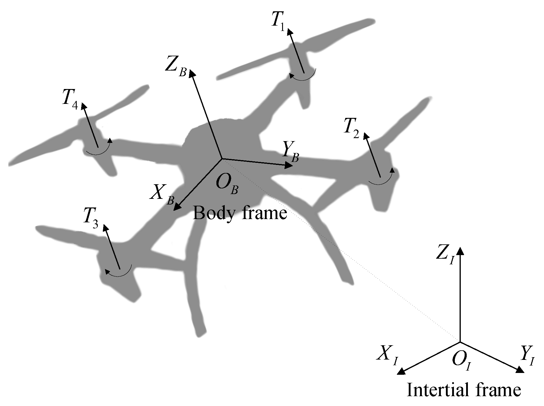
The quadrotor has four evenly spaced, cross-symmetrical brushless motors in the plane, The rotors of motor 1 and motor 3 rotate clockwise, while the rotors of motor 2 and motor 4 rotate counterclockwise. By changing the rotational speed of the four rotors, the quadrotor generates different magnitudes of lift forces and torques, which can control the takeoff, landing and attitude motions of the quadrotor. As a result, the location of the quadrotor can be altered in the three-dimensional space. Figure 1 depicts the basic structure of the quadrotor.

To clarify the mathematical model of the quadrotor system and satisfy the implementation of the control method, the earth-fixed inertial frame $O_I{X}_I{Y}_I{Z}_I$ and the body-fixed body frame $O_B{X}_B{Y}_B{Z}_B$ are established. To ensure that the constructed mathematical model does not lose the generality, it is assumed that the deformation and elastic vibration properties of the rotors and body are neglected, and the quadrotor is considered as an ideal rigid body; the quadrotor’s structure is symmetrical, its mass is uniformly distributed, and its center of mass is located at the geometric center. The translational and rotational motions of the quadrotor are satisfied by [25]

$$\dot{P}=v,$$

(1)

$$\dot{\Theta }=W_B^I\omega ,$$

(2)

where $P={[x,y,z]}^{\mathrm{T}}\in {\mathbb{R}}^3$ represents the position of the quadrotor in the inertial frame and $v={[v_x,v_y,v_z]}^{\mathrm{T}}\in {\mathbb{R}}^3$ represents the corresponding velocity. $\Theta ={[\varphi ,\theta ,\psi ]}^{\mathrm{T}}\in {\mathbb{R}}^3$ denotes the vector of Euler angles. $\omega ={[p,q,r]}^{\mathrm{T}}\in {\mathbb{R}}^3$ denotes the angular velocity of the quadrotor in the body frame. $W_B^I\in {\mathbb{R}}^{3\times 3}$ is the rotation matrix for the angular velocity in the form of

$$W_B^I=\left[\begin{array}{ccc}1& s_{\varphi }{t}_{\theta }& c_{\varphi }{t}_{\theta }\\ 0& c_{\varphi }& -s_{\varphi }\\ 0& s_{\varphi }/c_{\theta }& c_{\varphi }/c_{\theta }\end{array}\right],$$

(3)

in which $s_{\ast }=sin(\ast )$, $c_{\ast }=cos(\ast )$ and $t_{\ast }=tan(\ast )$.

Relying on the Newton–Euler method, the dynamical equation of quadrotor with compound disturbances is represented by [26]

$$m\dot{v}=F-kv+d_p,$$

(4)

$$I\dot{\omega }+\omega \times I\omega =\tau +d_a,$$

(5)

where $m\in \mathbb{R}$ represents the mass of the quadrotor. $I\in {\mathbb{R}}^{3\times 3}$ represents the inertia matrix of the quadrotor. As the assumptions of the quadrotor structure, its inertia matrix can be defined as the diagonal array $I\triangleq \mathrm{diag}\left\{I_{xx},I_{yy},I_{zz}\right\}$. $k=\mathrm{diag}\left\{k_x,k_y,k_z\right\}\in {\mathbb{R}}^{3\times 3}$ is the drag coefficient matrix. $F={[F_x,F_y,F_z]}^{\mathrm{T}}\in {\mathbb{R}}^3$ represents the resultant force consisting of the gravity and the total lift in the inertial frame. $\tau ={[{\tau }_x,{\tau }_y,{\tau }_z]}^{\mathrm{T}}\in {\mathbb{R}}^3$ represents the torque in the body frame. $d_p\in {\mathbb{R}}^3$ and $d_a\in {\mathbb{R}}^3$ are the compound disturbances in position and attitude dynamic models, which contain modeling uncertainties and external time-varying disturbances.

According to the mechanical analysis, the quadrotor is affected by gravity and lift forces. Since the special structure of the quadrotor, the lift forces are along the z-axis direction of the body frame. Then, the resultant force expressed in the inertial frame is [27]

$$F=R_B^I{z}_{u}T-z_{u}m{g}_I,$$

(6)

where $T\in \mathbb{R}$ represents the total lift force and $g_I\in \mathbb{R}$ represents the gravity acceleration. $z_u={[0,0,1]}^{\mathrm{T}}$. $R_B^I\in {\mathbb{R}}^{3\times 3}$ is the rotation matrix of the body frame transformed into the inertial frame in the form of

$$R_B^I=\left[\begin{array}{ccc}{c}_{\theta }{c}_{\psi }& s_{\varphi }{s}_{\theta }{c}_{\psi }-c_{\varphi }{s}_{\psi }& c_{\varphi }{s}_{\theta }{c}_{\psi }+s_{\varphi }{s}_{\psi }\\ c_{\theta }{s}_{\psi }& s_{\varphi }{s}_{\theta }{s}_{\psi }+c_{\varphi }{c}_{\psi }& c_{\varphi }{s}_{\theta }{s}_{\psi }-s_{\varphi }{c}_{\psi }\\ -s_{\theta }& s_{\varphi }{c}_{\theta }& c_{\varphi }{c}_{\theta }\end{array}\right].$$

(7)

Assumption 1

([28]). The pitch and roll angles hold the conditions $\left|\varphi \right|<\pi /2$ and $\left|\theta \right|<\pi /2$ to avoid the singularities of the matrices $W_B^I$ and $R_B^I$.

Assumption 2

([29]). In the control process, the total compound disturbance $d_t={\left[d_p^{\mathrm{T}},d_a^{\mathrm{T}}\right]}^{\mathrm{T}}\in {\mathbb{R}}^6$ has finite energy. In addition, $d_t$ is a continuous function and its norm is bounded such that $\parallel d_t\parallel \le d_{tM}$, where $d_{tM}$ is an unknown positive constant. Simultaneously, the compound disturbances are usually considered to be superimposed by the low-frequency period signals. Hence, it is assumed that the total compound disturbance has a low change rate and its rate of change is slow compared to the dynamic properties of the disturbance observer, which can be considered that ${\dot{d}}_t\simeq 0$.

Assumption 3

([30]). The desired trajectory of position $P_d={[x_d,y_d,z_d]}^{\mathrm{T}}\in {\mathbb{R}}^3$ and the desired trajectory of yaw angle ${\psi }_d\in \mathbb{R}$ and their higher order derivatives are known, continuous and bounded.

Remark 1.

Assumption 2 is common in control studies using disturbance observers [31,32,33], while there are different considerations for compound disturbances in [34]. In the case of this paper, the considerations in Assumption 2 are used. Assumption 3 ensures that the ADP method can be utilized for the control design and the stability analysis.

The total lift and torque of the quadrotor are related to the force and torque of the four rotors as follows [35]:

$$\left\{\begin{array}{c}T=T_1+T_2+T_3+T_1\hfill \\ {\tau }_x=l(T_2-T_4)\hfill \\ {\tau }_y=l(T_1-T_3)\hfill \\ {\tau }_z={\tau }_1-{\tau }_2+{\tau }_3-{\tau }_4\hfill \end{array}\right.,$$

(8)

where $T_i$ and ${\tau }_i$$(i=1,2,3,4)$ are the lift and torque generated by the four rotors of the quadrotor, respectively. l represents the length from each rotor to the center of the body.

The rotor speeds are related to pulse-width modulated (PWM) signals through the motors. The lift forces and torques generated by the four motors are related to the pulse width of the input signals as follows [36]:

$$\left\{\begin{array}{c}{T}_i=K_t\frac{B_w}{s+B_w}{u}_i\hfill \\ {\tau }_i=K_o\frac{B_w}{s+B_w}{u}_i\hfill \end{array}\right.,$$

(9)

where $K_t$ and $K_o$ are the positive gains of the lift coefficient and the inverse torque coefficient, respectively. $B_w$ is the motor bandwidth and $u_i$ represents the PWM signals of each corresponding motor, which should be limited between 0 and 1.

Assuming that the motors have a sufficiently fast response speed, then the motor model can be simplified as [37]

$$\left\{\begin{array}{c}{T}_i=K_t{u}_i\hfill \\ {\tau }_i=K_o{u}_i\hfill \end{array}\right..$$

(10)

Hence, (8) can be rewritten as [38]

$$\left[\begin{array}{c}T\\ {\tau }_x\\ {\tau }_y\\ {\tau }_z\end{array}\right]=\left[\begin{array}{cccc}{K}_t& K_t& K_t& K_t\\ 0& K_{t}l& 0& -K_{t}l\\ K_{t}l& 0& -K_{t}l& 0\\ K_o& -K_o& K_o& -K_o\end{array}\right]\left[\begin{array}{c}{u}_1\\ u_2\\ u_3\\ u_4\end{array}\right].$$

(11)

Considering the trajectory tracking control for the quadrotor, the control objective is to design a controller that allows the position and attitude to track the desired trajectory asymptotically within a small error.

Combining (1), (2), (4) and (5), the overall model of the quadrotor can be decomposed into a position subsystem and an attitude subsystem. The position subsystem can be represented as

$${\dot{x}}_1=f_1(x_1)+g_1(x_1)(F+d_p),$$

(12)

with

$$\begin{array}{cc}\hfill x_1=& {[P^{\mathrm{T}},v^{\mathrm{T}}]}^{\mathrm{T}}={[x,y,z,v_x,v_y,v_z]}^{\mathrm{T}}\in {\mathbb{R}}^6,\hfill \\ \hfill f_1(x_1)=& {[v_x,v_y,v_z,-k_x{v}_x/m,-k_y{v}_y/m,-k_z{v}_z/m]}^{\mathrm{T}}\in {\mathbb{R}}^6,\hfill \\ \hfill g_1(x_1)=& {\left[\begin{array}{cccccc}0& 0& 0& 1/m& 0& 0\\ 0& 0& 0& 0& 1/m& 0\\ 0& 0& 0& 0& 0& 1/m\end{array}\right]}^{\mathrm{T}}\in {\mathbb{R}}^{6\times 3}.\hfill \end{array}$$

While the attitude subsystem is expressed in the form of

$${\dot{x}}_2=f_2(x_2)+g_2(x_2)(\tau +d_a),$$

(13)

with

$$\begin{array}{cc}\hfill x_2=& {[{\Theta }^{\mathrm{T}},{\omega }^{\mathrm{T}}]}^{\mathrm{T}}={[\varphi ,\theta ,\psi ,p,q,r]}^{\mathrm{T}}\in {\mathbb{R}}^6,\hfill \\ \hfill f_2(x_2)=& [p+q{s}_{\varphi }{t}_{\theta }+r{c}_{\varphi }{t}_{\theta },q{c}_{\varphi }-r{s}_{\varphi },q{s}_{\varphi }/c_{\theta }+r{c}_{\varphi }/c_{\theta },\hfill \\ & qr(I_{yy}-I_{zz})/I_{xx},pr(I_{zz}-I_{xx})/I_{yy},pq(I_{xx}-I_{yy})/I_{zz}{]}^{\mathrm{T}}\in {\mathbb{R}}^6,\hfill \\ \hfill g_2(x_2)=& {\left[\begin{array}{cccccc}0& 0& 0& 1/I_{xx}& 0& 0\\ 0& 0& 0& 0& 1/I_{yy}& 0\\ 0& 0& 0& 0& 0& 1/I_{zz}\end{array}\right]}^{\mathrm{T}}\in {\mathbb{R}}^{6\times 3}.\hfill \end{array}$$

In the next section, (12) and (13) will be the focus of our research.

3. Robust Approximate Optimal Trajectory Tracking Control Design

Considering the convenience of describing the control design process, (12) and (13) is represented in the uniform form

$$\dot{X}=f(X)+g(X)(U+D),$$

(14)

in which $f(X)\in {\mathbb{R}}^6$ and $g(X)\in {\mathbb{R}}^{6\times 3}$ represent the drift dynamics and the input dynamics of the system, respectively. $X\in {\mathbb{R}}^6$ denotes the observable state vector, $U\in {\mathbb{R}}^3$ denotes the control input, and $D\in {\mathbb{R}}^3$ denotes the compound disturbance.

Definition 1

([39]). A state vector $\mathcal{X}$ is said to be uniformly ultimately bounded (UUB) if there exists a compact set ${Ø}_{\mathcal{X}}$, a positive number $b_{\mathcal{X}}$ and a time $t_b(\mathcal{X}(t_0),b_{\mathcal{X}})$ such that $\parallel \mathcal{X}\parallel \le b_{\mathcal{X}}$ for all state variable initial value $\mathcal{X}(t_0)\in {Ø}_{\mathcal{X}}$ and all $t\ge t_0+t_b$.

Lemma 1

([40]). $\mathcal{X}$ is UUB if the time derivative of a positive definite function $L_{\mathcal{X}}(\mathcal{X})$ is negative when $\parallel \mathcal{X}\parallel >b_{\mathcal{X}}$ for a positive constant $b_{\mathcal{X}}$.

To realize the trajectory tracking control with robustness for the system, the designed controller consists of two parts, the form of which is as follows:

$$U=U^N+U^R,$$

(15)

where $U^R$ is the robust compensation input designed through the disturbance observer for suppressing the effect of compound disturbances in the system. $U^N$ is the control input designed based on the ADP method for the nominal system, which takes the form of

$$U^N=U_d+U_E,$$

(16)

where $U_d$ represents the steady-state control input and $U_E$ represents the feedback control input.

3.1. Disturbance Observer Design

The disturbance observer is applied to derive the estimate of the compound disturbance. The estimated value is then used for the design of the robust compensation input to improve robustness. The disturbance observer is designed as

$$\left\{\begin{array}{c}\dot{Z}=-l_D(X)\left(f(X)+g(X)(p_D(X)+U+Z)\right)\hfill \\ \widehat{D}=Z+p_D(X)\hfill \end{array}\right.,$$

(17)

in which $\widehat{D}\in {\mathbb{R}}^3$ represents the estimate of the unknown compound disturbance, $p_D(X)\in {\mathbb{R}}^3$ represents the designed vector-valued function, $l_D(X)=\partial p_D(X)/\partial X\in {\mathbb{R}}^{3\times 6}$ is the observer gain and $Z\in {\mathbb{R}}^3$ represents the auxiliary variable vector of the disturbance observer.

Remark 2.

In the disturbance observer (17), the derivative of the state is required, which is unknown because the compound disturbance is unknown. Then, the auxiliary variable vector is given to avoid calculating the derivative of the state.

Define the estimation error of compound disturbance as $\tilde{D}=D-\widehat{D}$. With regard to Assumption 2 and the disturbance observer (17), the time derivative of $\tilde{D}$ is developed as

$$\begin{array}{cc}\hfill \dot{\tilde{D}}& =\dot{D}-\dot{\widehat{D}}=-\dot{Z}-l_D(X)\dot{X}\hfill \\ & =l_D(X)\left(f(X)+g(X)\left(p_D(X)+U+Z\right)\right)-l_D(X)\dot{X}\hfill \\ & =l_D(X)g(X)(Z+p_D(X))-l_D(X)\left(\dot{X}-f(X)-g(X)U\right).\hfill \end{array}$$

(18)

Combined with (14), we have

$$\begin{array}{cc}\hfill \dot{\tilde{D}}& =l_D(X)g(X)(Z+p_D(X))-l_D(X)g(X)D\hfill \\ & =-l_D(X)g(X)(D-\widehat{D})\hfill \\ & =-l_D(X)g(X)\tilde{D}.\hfill \end{array}$$

(19)

Then, $\tilde{D}$ is convergent by appropriately designing the vector-valued function $p_D(X)$.

Theorem 1.

Considering System (14), the disturbance observer is designed as (17). If $l_D(X)g(X)$ is ensured to be positive definite for the design of the vector-valued function $p_D(X)$, then the estimated compound disturbance $\widehat{D}$ would follow the compound disturbance D, which means the estimation error $\tilde{D}$ could converge to zero.

Proof. 

Select the candidate Lyapunov function as follows:

$$L_D=\frac{1}{2}{\tilde{D}}^{\mathrm{T}}\tilde{D}.$$

(20)

Combined with (18), the time derivative of $L_D$ is

$${\dot{L}}_D={\tilde{D}}^{\mathrm{T}}\dot{\tilde{D}}=-{\tilde{D}}^{\mathrm{T}}{l}_D(X)g(X)\tilde{D}.$$

(21)

In the case where $l_D(X)g(X)$ is positive definite, then we derive

$${\dot{L}}_D\le -\kappa {\parallel \tilde{D}\parallel }^2,$$

(22)

where $\kappa ={\lambda }_{min}\left(l_D(X)g(X)\right)$ and ${\lambda }_{min}(\ast )$ denotes the minimum eigenvalue. Obviously, ${\dot{L}}_D<0$ when $\tilde{D}\ne 0$. Hence, the disturbance observer (17) can estimate D and $\tilde{D}$ will converge to zero. This completes the proof. □

Then, the robust compensation input $U^R$ is designed as

$$U^R=-\widehat{D}.$$

(23)

3.2. Optimal Trajectory Tracking Control Design and Analysis

The compound disturbance is estimated by the disturbance observer. The robust compensation input is designed by the estimated value to suppress the effect of the compound disturbances. As a result, converting the trajectory tracking control problem of the nonlinear system with the compound disturbance into the trajectory tracking control problem of the nominal system is possible. In order to derive the optimal control for the nominal system, deriving the solution of the associated HJB equation is essential. Unfortunately, deriving the analytical solution is difficult for the nonlinear system by the direct solution method. Then, the ADP method is utilized for achieving the approximate optimal control by constructing the critic network. The weight update law designed for the critic network ensures the convergence of the weight and the stability of the closed-loop system.

For System (14), the nominal system is represented by

$$\dot{X}=f(X)+g(X)U.$$

(24)

Given the desired trajectory $X_d\in {\mathbb{R}}^6$, the steady-state control input $U_d$ is obtained from (24) as

$$U_d=g^{+}(X_d)\left({\dot{X}}_d-f(X_d)\right),$$

(25)

in which $g^{+}(X_d)$ denotes the pseudo-inverse of $g(X_d)$.

Define the tracking error as $E=X-X_d\in {\mathbb{R}}^6$. Combined with (14) and (15), the error system is developed as

$$\begin{array}{cc}\hfill \dot{E}=& f(X)+g(X)(U+D)-{\dot{X}}_d\hfill \\ \hfill =& f(E+X_d)+g(E+X_d)U_d-{\dot{X}}_d+g(E+X_d)U_E+g(E+X_d)\tilde{D}.\hfill \end{array}$$

(26)

Let $f_E=f(E+X_d)+g(E+X_d)U_d-{\dot{X}}_d$ and $g_E=g(E+X_d)$, then we have

$$\begin{array}{cc}\hfill \dot{E}=& f_E+g_E{U}_E+g_E\tilde{D}.\hfill \end{array}$$

(27)

Noting that $g_E=g(X)$, the norm of $g_E$ is bounded such that $g_m\le \parallel g_E\parallel \le g_M$ for the positive constants $g_m$ and $g_M$.

As a result of Theorem 1, the disturbance observer (20) can successfully estimate the compound disturbance D and the estimation error of compound disturbance $\tilde{D}$ can converge to zero. Therefore, it is possible to neglect $\tilde{D}$ in the error system (27) for the optimal control design [41,42]. However, $\tilde{D}$ would still be considered in the stability analysis. Then, the nominal error system is represented by

$$\dot{E}=f_E+g_E{U}_E.$$

(28)

Define the cost function as

$$V(E)={\int }_{t_0}^{\infty }\left(E^{\mathrm{T}}QE+U_E^{\mathrm{T}}R{U}_E\right)dt,$$

(29)

where $Q\in {\mathbb{R}}^{6\times 6}$ and $R\in {\mathbb{R}}^{3\times 3}$ are the designed symmetric positive definite matrices.

The nonlinear Lyapunov equation for (29) is achieved as

$$\nabla V^{\mathrm{T}}(f_E+g_E{U}_E)+E^{\mathrm{T}}QE+U_E^{\mathrm{T}}R{U}_E=0,$$

(30)

where $\nabla V=\partial V(E)/\partial E$ and $V(0)=0$.

Definition 2

([43]). A control policy $\mu (E)$ is said to be admissible on the compact set Ø for (29) if $\mu (E)$ is continuous on Ø, $\mu (0)=0$, $\mu (E)$ stabilizes (28) on Ø and $V(E)$ is finite $\forall E\in Ø$. This is represented by $\mu (E)\in \Psi (Ø)$, where $\Psi (Ø)$ denotes the set of admissible control policies.

The Hamiltonian function takes the following form

$$H\left(E,U_E,\nabla V\right)=\nabla V^{\mathrm{T}}(f_E+g_E{U}_E)+E^{\mathrm{T}}QE+U_E^{\mathrm{T}}R{U}_E.$$

(31)

The optimal cost function is represented by

$$V^{\ast }(E)=\underset{U_E\in \Psi (Ø)}{min}{\int }_{t_0}^{\infty }\left(E^{\mathrm{T}}QE+U_E^{\mathrm{T}}R{U}_E\right)dt,$$

(32)

and the following relation is satisfied

$$\underset{U_E\in \Psi (Ø)}{min}H\left(E,U_E,\nabla V^{\ast }\right)=0,$$

(33)

where $\nabla V^{\ast }=\partial V^{\ast }(E)/\partial E$.

Under the existence condition of the optimal solution $\partial H(E,U_E^{\ast },\nabla V^{\ast })/\partial U_E^{\ast }=2R{U}_E^{\ast }+g_E^{\mathrm{T}}\nabla V^{\ast }$$=0$, the optimal feedback control input is derived by

$$U_E^{\ast }=-\frac{1}{2}{R}^{-1}{g}_E^{\mathrm{T}}\nabla V^{\ast }.$$

(34)

Substituting (34) and (31) into (33), the HJB equation is developed as

$$\nabla V^{\ast \mathrm{T}}{f}_E+E^{\mathrm{T}}QE-\frac{1}{4}\nabla V^{\ast \mathrm{T}}{g}_E{R}^{-1}{g}_E^{\mathrm{T}}\nabla V^{\ast }=0.$$

(35)

3.3. Approximate Optimal Control Design

Clearly, it is necessary to derive $\nabla V^{\ast }$ by solving the HJB Equation (35) for deriving the optimal feedback control input (34). However, (35) is a typical nonlinear partial differential equation and its solution is difficult to derive in the analytic form [44,45]. To overcome the difficulty, the ADP method relying on the policy iteration technique is utilized to derive the approximate solution.

Assumption 4

([46]). The continuously differentiable Lyapunov function candidate $J(E)$ for the nominal error system (28) satisfies $\nabla J^{\mathrm{T}}(f_E+g_E{U}_E^{\ast })<0$, where $\nabla J=\partial J(E)/\partial E$. Meanwhile, there exists a symmetric positive definite matrix $\Lambda (E)$ such that $\nabla J^{\mathrm{T}}(f_E+g_E{U}_E^{\ast })=-\nabla J^{\mathrm{T}}\Lambda (E)\nabla J$. Moreover, the relation ${\Lambda }_m\le \parallel \Lambda (E)\parallel \le {\Lambda }_M$ holds for positive constants ${\Lambda }_m$, ${\Lambda }_M$.

Remark 3.

Assumption 4 is a common assumption that has been used for the ADP method. Generally, it is assumed that the closed-loop dynamics with the optimal feedback control is bounded by a function of the system state on the compact set. In such a situation, there exists a positive constant $\eta$ such that $∥f_E+g_E{U}_E^{\ast }∥\le \eta \parallel \nabla J\parallel$. Hence, we can further derive $∥\nabla J^{\mathrm{T}}(f_E+g_E{U}_E^{\ast })∥\le \eta {\parallel \nabla J\parallel }^2$. Furthermore, the function $J(E)$ can be correctly selected as a quadratic polynomial [47], such as $J(E)=\frac{1}{2}{E}^{\mathrm{T}}E$.

Considering the uniform estimation property of neural networks, the optimal cost function is approximated by

$$V^{\ast }(E)=W_c^{\mathrm{T}}{\phi }_c(E)+{\epsilon }_c(E),$$

(36)

where $W_c\in {\mathbb{R}}^N$ represents the unknown ideal constant weight, ${\phi }_c(E)\in {\mathbb{R}}^N$ represents the activation function, ${\epsilon }_c(E)$ represents the approximate error, and N represents the number of neurons. This neural network is called the critic network in the ADP method.

Lemma 2

([48]). The estimation error ${\epsilon }_c(E)$ is expected to be bounded when the approximated function $V^{\ast }(E)$ is bounded.

Then, by the definition of $\nabla V^{\ast }$, it is developed as follows

$$\nabla V^{\ast }=\nabla {\phi }_c^{\mathrm{T}}{W}_c+\nabla {\epsilon }_c,$$

(37)

where $\nabla {\phi }_c=\partial {\phi }_c(E)/\partial E$ and $\nabla {\epsilon }_c=\partial {\epsilon }_c(E)/\partial E$.

Invoking (37), the optimal feedback control input (34) is developed as

$$U_E^{\ast }=-\frac{1}{2}{R}^{-1}{g}_E^{\mathrm{T}}(\nabla {\phi }_c^{\mathrm{T}}{W}_c+\nabla {\epsilon }_c).$$

(38)

Substituting (37) into (35), the HJB equation is developed as

$$W_c^{\mathrm{T}}\nabla {\phi }_c{f}_E+E^{\mathrm{T}}QE-\frac{1}{4}{W}_c^{\mathrm{T}}\nabla {\phi }_c\Xi \nabla {\phi }_c^{\mathrm{T}}{W}_c+{\epsilon }_H=0,$$

(39)

where $\Xi =g_E{R}^{-1}{g}_E^{\mathrm{T}}$. ${\epsilon }_H$ represents the residual error, which takes the form of

$$\begin{array}{cc}\hfill {\epsilon }_H& =\nabla {\epsilon }_c^{\mathrm{T}}{f}_E-\frac{1}{2}\nabla {\epsilon }_c^{\mathrm{T}}\Xi \nabla {\phi }_c^{\mathrm{T}}{W}_c-\frac{1}{4}\nabla {\epsilon }_c^{\mathrm{T}}\Xi \nabla {\epsilon }_c\hfill \\ & =\nabla {\epsilon }_c^{\mathrm{T}}(f_E+g_E{U}_E^{\ast })+\frac{1}{4}\nabla {\epsilon }_c^{\mathrm{T}}\Xi \nabla {\epsilon }_c.\hfill \end{array}$$

(40)

Since $\parallel g_E\parallel$ is bounded, there exists the positive constants ${\Xi }_m$ and ${\Xi }_M$ such that ${\Xi }_m\le ∥\Xi ∥\le {\Xi }_M$.

Define the estimate of $W_c$ as ${\widehat{W}}_c$, then the estimate of $V^{\ast }(E)$ is derived as follows:

$$\widehat{V}(E)={\widehat{W}}_c^{\mathrm{T}}{\phi }_c(E).$$

(41)

Moreover, the approximate optimal feedback control input is derived as

$$U_E=-\frac{1}{2}{R}^{-1}{g}_E^{\mathrm{T}}\nabla {\phi }_c^{\mathrm{T}}{\widehat{W}}_c.$$

(42)

Remark 4.

The classical ADP method utilizes the critic network and the actor network to approximate the optimal cost function and the optimal feedback control, respectively [43,49,50]. Considering the association between the optimal cost function and the optimal feedback control for the continuous affine nonlinear system, it is possible to omit the actor network and only use the critic network [51,52]. This framework provides smaller computational effort, faster convergence and compared to the actor–critic network framework, which has a better practical value.

Combining (31), (41) and (42), the approximate Hamiltonian function is developed as

$$H\left(E,{\widehat{W}}_c\right)={\widehat{W}}_c^{\mathrm{T}}\nabla {\phi }_c{f}_E+E^{\mathrm{T}}QE-\frac{1}{4}{\widehat{W}}_c^{\mathrm{T}}\nabla {\phi }_c\Xi \nabla {\phi }_c^{\mathrm{T}}{\widehat{W}}_c\triangleq e_c.$$

(43)

Define the objective function as

$$E_c=\frac{1}{2}{e}_c^2.$$

(44)

Moreover, the weight update law is designed as

$${\dot{\widehat{W}}}_c=-\frac{{\alpha }_1\sigma }{{\sigma }_c^2}({\widehat{W}}_c^{\mathrm{T}}\nabla {\phi }_c{f}_E+E^{\mathrm{T}}QE-\frac{1}{4}{\widehat{W}}_c^{\mathrm{T}}\nabla {\phi }_c\Xi \nabla {\phi }_c^{\mathrm{T}}{\widehat{W}}_c)+\frac{{\alpha }_2}{2}\Pi (E,U_E)\nabla {\phi }_c\Xi \nabla J,$$

(45)

where ${\alpha }_1>0$, ${\alpha }_2>0$ are the learning rates to be designed. $\sigma =\nabla {\phi }_c(f_E+g_E{U}_E)$ and ${\sigma }_c={\sigma }^{\mathrm{T}}\sigma +1$. $\nabla J$ is given in Assumption 4. $\Pi (E,U_E)$ in the last term is defined as

$$\Pi (E,U_E)=\left\{\begin{array}{cc}0,\hfill & if\nabla J^{\mathrm{T}}(f_E+g_E{U}_E)+{\alpha }_3\nabla J^{\mathrm{T}}{g}_E{g}_E^{\mathrm{T}}\nabla J<0\hfill \\ 1,\hfill & else\hfill \end{array}\right.,$$

(46)

where ${\alpha }_3$ is a designed positive constant.

Remark 5.

The first term in (45) is employed for minimizing the objective function (44). To ensure that ${\widehat{W}}_c$ will converge to $W_c$, the existence of the persistence of excitation (PE) condition is essential during the learning process is necessary [49]. In addition, the probing noise is typically introduced to the control input for satisfying this condition, which may enable the closed-loop system to become unstable during the learning process [53,54]. The second term in (45) is employed for the stability of the closed-loop system.

Define the weight estimation error as ${\tilde{W}}_c=W_c-{\widehat{W}}_c$. Observing that ${\dot{\tilde{W}}}_c=-{\dot{\widehat{W}}}_c$, $\sigma =\nabla {\phi }_c(f_E+g_E{U}_E)=\nabla {\phi }_c{\dot{E}}^{\ast }+\frac{1}{2}\nabla {\phi }_c\Xi \nabla {\epsilon }_c+\frac{1}{2}\nabla {\phi }_c\Xi \nabla {\phi }_c^{\mathrm{T}}{\tilde{W}}_c$ where ${\dot{E}}^{\ast }=f_E+g_E{U}_E^{\ast }$, and using (39) and (45), we have

$$\begin{array}{cc}\hfill {\dot{\tilde{W}}}_c=& -\frac{{\alpha }_1}{{\sigma }_c^2}(\nabla {\phi }_c{\dot{E}}^{\ast }+\frac{1}{2}\nabla {\phi }_c\Xi \nabla {\epsilon }_c+\frac{1}{2}\nabla {\phi }_c\Xi \nabla {\phi }_c^{\mathrm{T}}{\tilde{W}}_c)({\tilde{W}}_c^{\mathrm{T}}\nabla {\phi }_c{\dot{E}}^{\ast }\hfill \\ & +\frac{1}{2}{\tilde{W}}_c^{\mathrm{T}}\nabla {\phi }_c\Xi \nabla {\epsilon }_c+\frac{1}{4}{\tilde{W}}_c^{\mathrm{T}}\nabla {\phi }_c\Xi \nabla {\phi }_c^{\mathrm{T}}{\tilde{W}}_c+{\epsilon }_H)-\frac{{\alpha }_2}{2}\Pi (E,U_E)\nabla {\phi }_c\Xi \nabla J.\hfill \end{array}$$

(47)

3.4. Stability Analysis

Assumption 5

([50]). The ideal weight $W_c$ have bound over the compact set Ø such that $∥W_c∥\le W_{cM}$ for a positive constant $W_{cM}$. Meanwhile, the activation function ${\phi }_c$ and the approximate error ${\epsilon }_c$ are bounded such that $∥{\phi }_c∥\le {\phi }_{cM}$, $∥{\epsilon }_c∥\le {\epsilon }_{cM}$ for positive constants ${\phi }_{cM}$ and ${\epsilon }_{cM}$, and their derivatives are also bounded such that $∥\nabla {\phi }_c∥\le {\overline{\phi }}_{cM}$ and $∥\nabla {\epsilon }_c∥\le {\overline{\epsilon }}_{cM}$ for positive constants ${\overline{\phi }}_{cM}$ and ${\overline{\epsilon }}_{cM}$. Moreover, the residual error ${\epsilon }_H$ will converge to zero when the number of neurons N is sufficiently large, as suggested by Remark 3 and the bound of $\parallel \Xi \parallel$. That is, the relation $\parallel {\epsilon }_H\parallel \le {\epsilon }_{HM}$ exists for the positive constant ${\epsilon }_{HM}$.

Theorem 2.

Considering System (14), the robust approximate optimal controller for the trajectory tracking control is designed as (15), which consists of the robust compensation input (23) and the nominal system control input (16), and the weight update law is designed as (45) for the critic network, then it is ensured that the tracking error E of the closed-loop system and the weight estimation error ${\tilde{W}}_c$ are UUB.

Proof. 

Select the candidate Lyapunov function as follows

$$L=L_D+L_J+L_W,$$

(48)

where $L_D$ is designed as (20), $L_J={\alpha }_{2}J(E)$ and $L_W=\frac{1}{2}{\tilde{W}}_c^{\mathrm{T}}{\tilde{W}}_c$.

Considering the second term in (48) and using (27), the time derivative is developed as

$${\dot{L}}_J={\alpha }_2\nabla J^{\mathrm{T}}(f_E+g_E{U}_E)+{\alpha }_2\nabla J^{\mathrm{T}}{g}_E\tilde{D}.$$

(49)

Considering the third term in (48) and according to (47), the time derivative is developed as

$$\begin{array}{cc}\hfill {\dot{L}}_W=& {\tilde{W}}_c^{\mathrm{T}}{\dot{\tilde{W}}}_c\hfill \\ \hfill =& -\frac{{\alpha }_1}{{\sigma }_c^2}({\tilde{W}}_c^{\mathrm{T}}\nabla {\phi }_c{\dot{E}}^{\ast }+\frac{1}{2}{\tilde{W}}_c^{\mathrm{T}}\nabla {\phi }_c\Xi \nabla {\epsilon }_c+\frac{1}{2}{\tilde{W}}_c^{\mathrm{T}}\nabla {\phi }_c\Xi \nabla {\phi }_c^{\mathrm{T}}{\tilde{W}}_c)({\tilde{W}}_c^{\mathrm{T}}\nabla {\phi }_c{\dot{E}}^{\ast }\hfill \\ & +\frac{1}{2}{\tilde{W}}_c^{\mathrm{T}}\nabla {\phi }_c\Xi \nabla {\epsilon }_c+\frac{1}{4}{\tilde{W}}_c^{\mathrm{T}}\nabla {\phi }_c\Xi \nabla {\phi }_c^{\mathrm{T}}{\tilde{W}}_c+{\epsilon }_H)-\frac{{\alpha }_2}{2}\Pi (E,U_E){\tilde{W}}_c^{\mathrm{T}}\nabla {\phi }_c\Xi \nabla J\hfill \\ \hfill =& -\frac{{\alpha }_1}{{\sigma }_c^2}{({\tilde{W}}_c^{\mathrm{T}}\nabla {\phi }_c{\dot{E}}^{\ast })}^2-\frac{{\alpha }_1}{4{\sigma }_c^2}{({\tilde{W}}_c^{\mathrm{T}}\nabla {\phi }_c\Xi \nabla {\epsilon }_c)}^2-\frac{{\alpha }_1}{8{\sigma }_c^2}{({\tilde{W}}_c^{\mathrm{T}}\nabla {\phi }_c\Xi \nabla {\phi }_c^{\mathrm{T}}{\tilde{W}}_c)}^2\hfill \\ & -\frac{{\alpha }_1}{{\sigma }_c^2}({\tilde{W}}_c^{\mathrm{T}}\nabla {\phi }_c{\dot{E}}^{\ast })({\tilde{W}}_c^{\mathrm{T}}\nabla {\phi }_c\Xi \nabla {\epsilon }_c)-\frac{3{\alpha }_1}{4{\sigma }_c^2}({\tilde{W}}_c^{\mathrm{T}}\nabla {\phi }_c{\dot{E}}^{\ast })({\tilde{W}}_c^{\mathrm{T}}\nabla {\phi }_c\Xi \nabla {\phi }_c^{\mathrm{T}}{\tilde{W}}_c)\hfill \\ & -\frac{3{\alpha }_1}{8{\sigma }_c^2}({\tilde{W}}_c^{\mathrm{T}}\nabla {\phi }_c\Xi \nabla {\epsilon }_c)({\tilde{W}}_c^{\mathrm{T}}\nabla {\phi }_c\Xi \nabla {\phi }_c^{\mathrm{T}}{\tilde{W}}_c)-\frac{{\alpha }_1}{{\sigma }_c^2}{\tilde{W}}_c^{\mathrm{T}}\nabla {\phi }_c{\dot{E}}^{\ast }{\epsilon }_H\hfill \\ & -\frac{{\alpha }_1}{2{\sigma }_c^2}{\tilde{W}}_c^{\mathrm{T}}\nabla {\phi }_c\Xi \nabla {\epsilon }_c{\epsilon }_H-\frac{{\alpha }_1}{2{\sigma }_c^2}{\tilde{W}}_c^{\mathrm{T}}\nabla {\phi }_c\Xi \nabla {\phi }_c^{\mathrm{T}}{\tilde{W}}_c{\epsilon }_H-\frac{{\alpha }_2}{2}\Pi (E,U_E){\tilde{W}}_c^{\mathrm{T}}\nabla {\phi }_c\Xi \nabla J.\hfill \end{array}$$

(50)

Since the first two terms in the final form of (50) are negative semi-definite, we then derive

$$\begin{array}{cc}\hfill {\dot{L}}_W\le & -\frac{{\alpha }_1}{8{\sigma }_c^2}{({\tilde{W}}_c^{\mathrm{T}}\nabla {\phi }_c\Xi \nabla {\phi }_c^{\mathrm{T}}{\tilde{W}}_c)}^2-\frac{{\alpha }_1}{{\sigma }_c^2}({\tilde{W}}_c^{\mathrm{T}}\nabla {\phi }_c{\dot{E}}^{\ast })({\tilde{W}}_c^{\mathrm{T}}\nabla {\phi }_c\Xi \nabla {\epsilon }_c)\hfill \\ & -\frac{3{\alpha }_1}{4{\sigma }_c^2}({\tilde{W}}_c^{\mathrm{T}}\nabla {\phi }_c{\dot{E}}^{\ast })({\tilde{W}}_c^{\mathrm{T}}\nabla {\phi }_c\Xi \nabla {\phi }_c^{\mathrm{T}}{\tilde{W}}_c)\hfill \\ & -\frac{3{\alpha }_1}{8{\sigma }_c^2}({\tilde{W}}_c^{\mathrm{T}}\nabla {\phi }_c\Xi \nabla {\epsilon }_c)({\tilde{W}}_c^{\mathrm{T}}\nabla {\phi }_c\Xi \nabla {\phi }_c^{\mathrm{T}}{\tilde{W}}_c)-\frac{{\alpha }_1}{{\sigma }_c^2}{\tilde{W}}_c^{\mathrm{T}}\nabla {\phi }_c{\dot{E}}^{\ast }{\epsilon }_H\hfill \\ & -\frac{{\alpha }_1}{2{\sigma }_c^2}{\tilde{W}}_c^{\mathrm{T}}\nabla {\phi }_c\Xi \nabla {\epsilon }_c{\epsilon }_H-\frac{{\alpha }_1}{2{\sigma }_c^2}{\tilde{W}}_c^{\mathrm{T}}\nabla {\phi }_c\Xi \nabla {\phi }_c^{\mathrm{T}}{\tilde{W}}_c{\epsilon }_H-\frac{{\alpha }_2}{2}\Pi (E,U_E){\tilde{W}}_c^{\mathrm{T}}\nabla {\phi }_c\Xi \nabla J.\hfill \end{array}$$

(51)

According to Remark 3 and Assumption 5, and considering the bound of $\parallel \Xi \parallel$, we assume that ${\lambda }_{1m}\le ∥\nabla {\phi }_c\Xi \nabla {\phi }_c^{\mathrm{T}}∥\le {\lambda }_{1M}$, $\parallel \Xi \parallel \le {\lambda }_2$, $\parallel \nabla {\phi }_c{\dot{E}}^{\ast }\parallel \le {\lambda }_3$, $\parallel \nabla {\epsilon }_c\parallel \le {\lambda }_4$, $\parallel \nabla {\phi }_c\Xi \nabla {\epsilon }_c\parallel \le {\lambda }_5$ and $\parallel {\epsilon }_H\parallel \le {\lambda }_6$. Noticing that the PE condition guarantees ${\sigma }_c$ to be bounded, there exists a positive constant ${\lambda }_7$ such that ${\lambda }_7\le 1/{\sigma }_c^2\le 1$. In addition, based on Young’s inequality, there exists the relation $-ab\le \frac{1}{2}(c^2{a}^2+\frac{b^2}{c^2})$, where c is a nonzero constant. Then, we have

$$-\frac{{\alpha }_1}{8{\sigma }_c^2}{({\tilde{W}}_c^{\mathrm{T}}\nabla {\phi }_c\Xi \nabla {\phi }_c^{\mathrm{T}}{\tilde{W}}_c)}^2\le -\frac{{\alpha }_1}{8}{\lambda }_7{\lambda }_{1m}^2{\parallel {\tilde{W}}_c\parallel }^4,$$

(52)

$$\begin{array}{cc}\hfill -\frac{{\alpha }_1}{{\sigma }_c^2}({\tilde{W}}_c^{\mathrm{T}}\nabla {\phi }_c{\dot{E}}^{\ast })({\tilde{W}}_c^{\mathrm{T}}\nabla {\phi }_c\Xi \nabla {\epsilon }_c)\le & \frac{{\alpha }_1}{2{\sigma }_c^2}\left(c_1^2{({\tilde{W}}_c^{\mathrm{T}}\nabla {\phi }_c{\dot{E}}^{\ast })}^2+\frac{{({\tilde{W}}_c^{\mathrm{T}}\nabla {\phi }_c\Xi \nabla {\epsilon }_c)}^2}{c_1^2}\right)\hfill \\ \hfill \le & \frac{{\alpha }_1{c}_1^2}{2}{\lambda }_3^2\parallel {\tilde{W}}_c{\parallel }^2+\frac{{\alpha }_1}{2c_1^2}{\lambda }_5^2{\parallel {\tilde{W}}_c\parallel }^2,\hfill \end{array}$$

(53)

$$\begin{array}{cc}\hfill -\frac{3{\alpha }_1}{4{\sigma }_c^2}({\tilde{W}}_c^{\mathrm{T}}\nabla {\phi }_c{\dot{E}}^{\ast })({\tilde{W}}_c^{\mathrm{T}}\nabla {\phi }_c\Xi \nabla {\phi }_c^{\mathrm{T}}{\tilde{W}}_c)\le & \frac{3{\alpha }_1}{8{\sigma }_c^2}\left(c_2^2{({\tilde{W}}_c^{\mathrm{T}}\nabla {\phi }_c{\dot{E}}^{\ast })}^2+\frac{{({\tilde{W}}_c^{\mathrm{T}}\nabla {\phi }_c\Xi \nabla {\phi }_c^{\mathrm{T}}{\tilde{W}}_c)}^2}{c_2^2}\right)\hfill \\ \hfill \le & \frac{3{\alpha }_1{c}_2^2}{8}{\lambda }_3^2\parallel {\tilde{W}}_c{\parallel }^2+\frac{3{\alpha }_1}{8c_2^2}{\lambda }_{1M}^2{\parallel {\tilde{W}}_c\parallel }^4,\hfill \end{array}$$

(54)

$$\begin{array}{cc}\hfill -\frac{3{\alpha }_1}{8{\sigma }_c^2}({\tilde{W}}_c^{\mathrm{T}}\nabla {\phi }_c\Xi \nabla {\epsilon }_c)({\tilde{W}}_c^{\mathrm{T}}\nabla {\phi }_c\Xi \nabla {\phi }_c^{\mathrm{T}}{\tilde{W}}_c)\le & \frac{3{\alpha }_1}{16{\sigma }_c^2}\left(c_3^2{({\tilde{W}}_c^{\mathrm{T}}\nabla {\phi }_c\Xi \nabla {\epsilon }_c)}^2+\frac{{({\tilde{W}}_c^{\mathrm{T}}\nabla {\phi }_c\Xi \nabla {\phi }_c^{\mathrm{T}}{\tilde{W}}_c)}^2}{c_3^2}\right)\hfill \\ \hfill \le & \frac{3{\alpha }_1{c}_3^2}{16}{\lambda }_5^2\parallel {\tilde{W}}_c{\parallel }^2+\frac{3{\alpha }_1}{16c_3^2}{\lambda }_{1M}^2{\parallel {\tilde{W}}_c\parallel }^4,\hfill \end{array}$$

(55)

$$\begin{array}{cc}\hfill -\frac{{\alpha }_1}{{\sigma }_c^2}{\tilde{W}}_c^{\mathrm{T}}\nabla {\phi }_c{\dot{E}}^{\ast }{\epsilon }_H\le & \frac{{\alpha }_1}{2{\sigma }_c^2}\left(c_4^2{({\tilde{W}}_c^{\mathrm{T}}\nabla {\phi }_c{\dot{E}}^{\ast })}^2+\frac{{\epsilon }_H^2}{c_4^2}\right)\hfill \\ \hfill \le & \frac{{\alpha }_1{c}_4^2}{2}{\lambda }_3^2{\parallel {\tilde{W}}_c\parallel }^2+\frac{{\alpha }_1}{2c_4^2}{\lambda }_6^2,\hfill \end{array}$$

(56)

$$\begin{array}{cc}\hfill -\frac{{\alpha }_1}{2{\sigma }_c^2}{\tilde{W}}_c^{\mathrm{T}}\nabla {\phi }_c\Xi \nabla {\epsilon }_c{\epsilon }_H\le & \frac{{\alpha }_1}{4{\sigma }_c^2}\left(c_5^2{({\tilde{W}}_c^{\mathrm{T}}\nabla {\phi }_c\Xi \nabla {\epsilon }_c)}^2+\frac{{\epsilon }_H^2}{c_5^2}\right)\hfill \\ \hfill \le & \frac{{\alpha }_1{c}_5^2}{4}{\lambda }_5^2{\parallel {\tilde{W}}_c\parallel }^2+\frac{{\alpha }_1}{4c_5^2}{\lambda }_6^2,\hfill \end{array}$$

(57)

$$\begin{array}{cc}\hfill -\frac{{\alpha }_1}{2{\sigma }_c^2}{\tilde{W}}_c^{\mathrm{T}}\nabla {\phi }_c\Xi \nabla {\phi }_c^{\mathrm{T}}{\tilde{W}}_c{\epsilon }_H\le & \frac{{\alpha }_1}{4{\sigma }_c^2}\left(c_6^2{({\tilde{W}}_c^{\mathrm{T}}\nabla {\phi }_c\Xi \nabla {\phi }_c^{\mathrm{T}}{\tilde{W}}_c)}^2+\frac{{\epsilon }_H^2}{c_6^2}\right)\hfill \\ \hfill \le & \frac{{\alpha }_1{c}_6^2}{4}{\lambda }_{1M}^2{\parallel {\tilde{W}}_c\parallel }^4+\frac{{\alpha }_1}{4c_6^2}{\lambda }_6^2.\hfill \end{array}$$

(58)

Then, (51) is developed as

$${\dot{L}}_W\le -{\alpha }_1{\lambda }_8\parallel {\tilde{W}}_c{\parallel }^4+{\alpha }_1{\lambda }_9{\parallel {\tilde{W}}_c\parallel }^2+{\alpha }_1{\lambda }_{10}-\frac{{\alpha }_2}{2}\Pi (E,U_E){\tilde{W}}_c^{\mathrm{T}}\nabla {\phi }_c\Xi \nabla J,$$

(59)

where

$$\begin{array}{cc}\hfill {\lambda }_8=& \frac{1}{8}{\lambda }_7{\lambda }_{1m}^2-\frac{3}{8c_2^2}{\lambda }_{1M}^2-\frac{3}{16c_3^2}{\lambda }_{1M}^2-\frac{c_6^2}{4}{\lambda }_{1M}^2,\hfill \\ \hfill {\lambda }_9=& \frac{c_1^2}{2}{\lambda }_3^2+\frac{1}{2c_1^2}{\lambda }_5^2+\frac{3c_2^2}{8}{\lambda }_3^2+\frac{3c_3^2}{16}{\lambda }_5^2+\frac{c_4^2}{2}{\lambda }_3^2+\frac{c_5^2}{4}{\lambda }_5^2,\hfill \\ \hfill {\lambda }_{10}=& \frac{1}{2c_4^2}{\lambda }_6^2+\frac{1}{4c_5^2}{\lambda }_6^2+\frac{1}{4c_6^2}{\lambda }_6^2,\hfill \end{array}$$

(60)

and $c_j$$(j=1,2,...,6)$ are all non-zero constants whose selection guarantees ${\lambda }_8>0$. Combining the results of (22), (49) and (51), we have

$$\begin{array}{cc}\hfill \dot{L}=& {\dot{L}}_D+{\dot{L}}_J+{\dot{L}}_W\hfill \\ \hfill \le & -\kappa \parallel \tilde{D}{\parallel }^2+{\alpha }_2\nabla J^{\mathrm{T}}(f_E+g_E{U}_E)+{\alpha }_2\nabla J^{\mathrm{T}}{g}_E\tilde{D}-{\alpha }_1{\lambda }_8{\parallel {\tilde{W}}_c\parallel }^4\hfill \\ & +{\alpha }_1{\lambda }_9{\parallel {\tilde{W}}_c\parallel }^2+{\alpha }_1{\lambda }_{10}-\frac{{\alpha }_2}{2}\Pi (E,U_E){\tilde{W}}_c^{\mathrm{T}}\nabla {\phi }_c\Xi \nabla J.\hfill \end{array}$$

(61)

By using Young’s inequality, the relation ${\alpha }_2\nabla J^{\mathrm{T}}{g}_E\tilde{D}\le \frac{{\alpha }_2{\alpha }_3}{2}\nabla J^{\mathrm{T}}{g}_E{g}_E^{\mathrm{T}}\nabla J+\frac{{\alpha }_2}{2{\alpha }_3}{\parallel \tilde{D}\parallel }^2$ exists. Then, (61) is developed as

$$\begin{array}{cc}\hfill \dot{L}\le & -(\kappa -\frac{{\alpha }_2}{2{\alpha }_3}){\parallel \tilde{D}\parallel }^2+{\alpha }_2\nabla J^{\mathrm{T}}(f_E+g_E{U}_E)+\frac{{\alpha }_2{\alpha }_3}{2}\nabla J^{\mathrm{T}}{g}_E{g}_E^{\mathrm{T}}\nabla J\hfill \\ & -{\alpha }_1{\lambda }_8\parallel {\tilde{W}}_c{\parallel }^4+{\alpha }_1{\lambda }_9{\parallel {\tilde{W}}_c\parallel }^2+{\alpha }_1{\lambda }_{10}-\frac{{\alpha }_2}{2}\Pi (E,U_E){\tilde{W}}_c^{\mathrm{T}}\nabla {\phi }_c\Xi \nabla J.\hfill \end{array}$$

(62)

The following discussion is divided into two cases.

Case 1.

In this case, $\Pi (E,U_E)=0$. Since $\nabla J^{\mathrm{T}}(f_E+g_E{U}_E)+{\alpha }_3\nabla J^{\mathrm{T}}{g}_E{g}_E^{\mathrm{T}}\nabla J<0$, we can derive that $\nabla J^{\mathrm{T}}(f_E+g_E{U}_E)<0$. According to the dense property of $\mathbb{R}$, there exists a positive constant ${\lambda }_{11}$ such that $0<{\lambda }_{11}\parallel \nabla J\parallel \le -\nabla J^{\mathrm{T}}(f_E+g_E{U}_E)$ for all $E\in Ø$. Then, (62) becomes

$$\dot{L}\le -(\kappa -\frac{{\alpha }_2}{2{\alpha }_3})\parallel \tilde{D}{\parallel }^2-\frac{{\alpha }_2}{2}{\lambda }_{11}\parallel \nabla J\parallel -{\alpha }_1{\lambda }_8\parallel {\tilde{W}}_c{\parallel }^4+{\alpha }_1{\lambda }_9{\parallel {\tilde{W}}_c\parallel }^2+{\alpha }_1{\lambda }_{10}.$$

(63)

By selecting ${\alpha }_2$ and ${\alpha }_3$, such that $\kappa -\frac{{\alpha }_2}{2{\alpha }_3}>0$, then $\dot{L}<0$ is satisfied provided that one of the following conditions holds:

$$∥\nabla J∥>\frac{{\alpha }_1\left(4{\lambda }_8{\lambda }_{10}+{\lambda }_9^2\right)}{2{\alpha }_2{\lambda }_8{\lambda }_{11}}\triangleq {\ell }_1,$$

(64)

or

$$∥{\tilde{W}}_c∥>\sqrt{\frac{{\lambda }_9+\sqrt{4{\lambda }_8{\lambda }_{10}+{\lambda }_9^2}}{2{\lambda }_8}}\triangleq {\hslash }_1.$$

(65)

Case 2.

Considering the case $\Pi (E,U_E)=1$, (62) is developed as

$$\begin{array}{cc}\hfill \dot{L}\le & {\alpha }_2\left(\nabla J^{\mathrm{T}}(f_E+g_E{U}_E)+\frac{{\alpha }_3}{2}\nabla J^{\mathrm{T}}{g}_E{g}_E^{\mathrm{T}}\nabla J\right)-(\kappa -\frac{{\alpha }_2}{2{\alpha }_3}){\parallel \tilde{D}\parallel }^2\hfill \\ & -{\alpha }_1{\lambda }_8\parallel {\tilde{W}}_c{\parallel }^4+{\alpha }_1{\lambda }_9{\parallel {\tilde{W}}_c\parallel }^2+{\alpha }_1{\lambda }_{10}-\frac{{\alpha }_2}{2}{\tilde{W}}_c^{\mathrm{T}}\nabla {\phi }_c\Xi \nabla J\hfill \\ \hfill =& {\alpha }_2\left(\nabla J^{\mathrm{T}}(f_E+g_E{U}_E^{\ast })+\frac{{\alpha }_3}{2}\nabla J^{\mathrm{T}}{g}_E{g}_E^{\mathrm{T}}\nabla J\right)+\frac{{\alpha }_2}{2}\nabla J^{\mathrm{T}}\Xi \nabla {\epsilon }_c\hfill \\ & -(\kappa -\frac{{\alpha }_2}{2{\alpha }_3})\parallel \tilde{D}{\parallel }^2-{\alpha }_1{\lambda }_8\parallel {\tilde{W}}_c{\parallel }^4+{\alpha }_1{\lambda }_9{\parallel {\tilde{W}}_c\parallel }^2+{\alpha }_1{\lambda }_{10}.\hfill \end{array}$$

(66)

Based on Assumption 4, and considering $∥g_E∥\le g_M$, we have

$$\begin{array}{cc}\hfill \dot{L}\le & -{\alpha }_2({\Lambda }_m-\frac{{\alpha }_3}{2}{g}_M^2){∥\nabla J∥}^2+\frac{{\alpha }_2}{2}{\lambda }_2{\lambda }_4∥\nabla J∥-(\kappa -\frac{{\alpha }_2}{2{\alpha }_3}){\parallel \tilde{D}\parallel }^2\hfill \\ & -{\alpha }_1{\lambda }_8\parallel {\tilde{W}}_c{\parallel }^4+{\alpha }_1{\lambda }_9{\parallel {\tilde{W}}_c\parallel }^2+{\alpha }_1{\lambda }_{10}.\hfill \end{array}$$

(67)

Similarly, by selecting ${\alpha }_2$ and ${\alpha }_3$ such that ${\lambda }_{12}={\Lambda }_m-\frac{{\alpha }_3}{2}{g}_M^2>0$ and $\kappa -\frac{{\alpha }_2}{2{\alpha }_3}>0$, then it means that $\dot{L}<0$ holds as long as

$$∥\nabla J∥>\frac{{\lambda }_2{\lambda }_4}{4{\lambda }_{12}}+\sqrt{\frac{{\alpha }_1\left(4{\lambda }_8{\lambda }_{10}+{\lambda }_9^2\right)}{4{\alpha }_2{\lambda }_8{\lambda }_{12}}+\frac{{\lambda }_2^2{\lambda }_4^2}{16{\lambda }_{12}^2}}\triangleq {\ell }_2,$$

(68)

or

$$∥{\tilde{W}}_c∥>\sqrt{\frac{{\lambda }_9}{2{\lambda }_8}+\sqrt{\frac{{\lambda }_{10}}{{\lambda }_8}+\frac{{\lambda }_9^2}{4{\lambda }_8^2}+\frac{{\alpha }_2{\lambda }_2^2{\lambda }_4^2}{16{\alpha }_1{\lambda }_8{\lambda }_{12}}}}\triangleq {\hslash }_2.$$

(69)

In conclusion, $\dot{L}<0$ when $∥\nabla J∥>max\left\{{\ell }_1,{\ell }_2\right\}$ or $∥{\tilde{W}}_c∥>max\left\{{\hslash }_1,{\hslash }_2\right\}$. Relying on Lemma 1 and the standard Lyapunov extension theorem [55], it is further concluded that the tracking error E of the closed-loop system and the weight estimation error ${\tilde{W}}_c$ are UUB. This completes the proof. □

Remark 6.

As a result of Theorem 2, the approximate optimal cost function $\widehat{V}(E)$ in (41) and the approximate optimal feedback control input $U_E$ in (42) can, respectively, converge to the neighborhoods of the optimal cost function $V^{\ast }(E)$ and the optimal feedback control input $U_E^{\ast }$ within finite bounds when the PE condition holds [41].

4. Robust Approximate Optimal Trajectory Tracking Control for a Quadrotor

Position and yaw angle are the system outputs for the quadrotor that tracks the desired trajectory of position and the desired trajectory of yaw angle. The desired trajectories of roll and pitch angles required by the attitude subsystem are generated according to the position subsystem control inputs. The tracking errors in lateral and longitudinal positions are eliminated by the attitude subsystem tracking the desired trajectories of roll and pitch angles. According to the description of the control design in the previous section, the control design for the quadrotor is shown in Figure 2, which can guarantee that the tracking error of the quadrotor remains within a small range.

4.1. Position Control Design

The estimated value of unknown compound disturbance ${\widehat{d}}_p$ in the position subsystem is derived by the following disturbance observer

$$\left\{\begin{array}{c}{\dot{z}}_1=-l_1(x_1)\left(f_1(x_1)+g_1(x_1)(p_1(x_1)+F+z_1)\right)\hfill \\ {\widehat{d}}_p=z_1+p_1(x_1)\hfill \end{array}\right.,$$

(70)

where $l_1(x_1)=\partial p_1(x_1)/\partial x_1$ denotes the observer gain of the disturbance observer in the position subsystem and F is derived by (6). Then, the position subsystem robust compensation input is designed as

$$F^R=-{\widehat{d}}_p.$$

(71)

The steady-state control input for the position nominal system is designed as

$$F_d=g_1^{+}(x_{1d})\left({\dot{x}}_{1d}-f_1(x_{1d})\right),$$

(72)

where $x_{1d}={[P_d^{\mathrm{T}},v_d^{\mathrm{T}}]}^{\mathrm{T}}\in {\mathbb{R}}^6$ and $v_d={[v_{xd},v_{yd},v_{zd}]}^{\mathrm{T}}={\dot{P}}_d\in {\mathbb{R}}^3$. $g_1^{+}(x_{1d})$ denotes the pseudo-inverse of $g_1(x_{1d})$. Then, define the position subsystem tracking error as

$$e_1=x_1-x_{1d}\triangleq {[e_x,e_y,e_z,e_{v_x},e_{v_y},e_{v_z}]}^{\mathrm{T}}\in {\mathbb{R}}^6.$$

(73)

The cost function of the position subsystem is represented as

$$V_1(e_1)={\int }_{t_0}^{\infty }\left(e_1^{\mathrm{T}}{Q}_1{e}_1+F_e^{\mathrm{T}}{R}_1{F}_e\right)dt,$$

(74)

where $Q_1\in {\mathbb{R}}^{6\times 6}$ and $R_1\in {\mathbb{R}}^{3\times 3}$ are the designed symmetric definite matrices. The approximate optimal feedback control input in the position subsystem is

$$F_e=-\frac{1}{2}{R}_1^{-1}{g}_{e1}^{\mathrm{T}}\nabla {\phi }_{c1}^{\mathrm{T}}{\widehat{W}}_{c1},$$

(75)

where $g_{e1}=g_1(x_1)$ and $\nabla {\phi }_{c1}=\partial {\phi }_{c1}(e_1)/\partial e_1$. ${\phi }_{c1}(e_1)$ is the activation function and ${\widehat{W}}_{c1}$ represents the estimate of the ideal weight for the critic network of the position subsystem. The corresponding weight update law is designed as

$$\begin{array}{cc}\hfill {\dot{\widehat{W}}}_{c1}=& -\frac{{\alpha }_{11}{\sigma }_1}{{\sigma }_{c1}^2}(e_1^{\mathrm{T}}{Q}_1{e}_1+{\widehat{W}}_{c1}^{\mathrm{T}}\nabla {\phi }_{c1}{f}_{e1}-\frac{1}{4}{\widehat{W}}_{c1}^{\mathrm{T}}\nabla {\phi }_{c1}{\Xi }_1\nabla {\phi }_{c1}^{\mathrm{T}}{\widehat{W}}_{c1})\hfill \\ & +\frac{{\alpha }_{12}}{2}\Pi (e_1,F_e)\nabla {\phi }_{c1}{\Xi }_1\nabla J_1,\hfill \end{array}$$

(76)

where ${\alpha }_{11}>0$, ${\alpha }_{12}>0$ are the designed learning rates. ${\sigma }_1=\nabla {\phi }_{c1}(f_{e1}+g_{e1}{F}_e)$, ${\sigma }_{c1}={\sigma }_1^{\mathrm{T}}{\sigma }_1+1$ and ${\Xi }_1=g_{e1}{R}_1^{-1}{g}_{e1}^{\mathrm{T}}$. $\nabla J_1=\partial J_1(e_1)/\partial e_1$, where $J_1(e_1)$ is the Lyapunov function candidate that satisfies Assumption 4.

Then, the robust approximate optimal trajectory tracking control in the position subsystem is designed as

$$F=F^N+F^R=F_d+F_e+F^R.$$

(77)

4.2. Attitude Resolution

Since the system of the quadrotor is underactuated and strongly coupled, the information of the position subsystem is used to calculate the total lift force. The desired trajectories of roll and pitch angles are determined by the position subsystem through the relation between the kinematic equation and the Euler equation and passed to the attitude subsystem. For the position subsystem, the generated tracking error and the received compound disturbance can be eliminated by the attitude subsystem. By a matrix operation on (6), the following equations are derived:

$$\begin{array}{cc}\hfill & F_x=T(c_{\varphi }{s}_{\theta }{c}_{\psi }+s_{\varphi }{s}_{\psi }),\hfill \\ & F_y=T(c_{\varphi }{s}_{\theta }{s}_{\psi }-s_{\varphi }{c}_{\psi }),\hfill \\ & F_z=T{c}_{\varphi }{c}_{\theta }-m{g}_I.\hfill \end{array}$$

(78)

The actual total lift force for the quadrotor system is designed as

$$T=(F_z+m{g}_I)/c_{\varphi }{c}_{\theta }.$$

(79)

Substituting (79) into (78), the form is transformed as

$$\left[\begin{array}{c}{F}_x\\ F_y\end{array}\right]=(F_z+m{g}_I)\left[\begin{array}{cc}{c}_{\psi }& s_{\psi }\\ s_{\psi }& -c_{\psi }\end{array}\right]\left[\begin{array}{c}{t}_{\theta }\\ t_{\varphi }/c_{\theta }\end{array}\right].$$

(80)

The desired trajectories of the pitch and roll angles are derived by the following equations:

$$\begin{array}{cc}\hfill & F_x{c}_{\psi }+F_y{s}_{\psi }=(F_z+m{g}_I)t_{{\theta }_d},\hfill \\ & F_x{s}_{\psi }-F_y{c}_{\psi }=(F_z+m{g}_I)\frac{t_{{\varphi }_d}}{c_{\theta }}.\hfill \end{array}$$

(81)

Then, we have

$$\begin{array}{cc}\hfill & {\theta }_d=arctan(\frac{F_x{c}_{\psi }+F_y{s}_{\psi }}{F_z+m{g}_I}),\hfill \\ & {\varphi }_d=arctan(c_{\theta }\frac{F_x{s}_{\psi }-F_y{c}_{\psi }}{F_z+m{g}_I}).\hfill \end{array}$$

(82)

4.3. Attitude Control Design

Similarly, the estimated value of unknown compound disturbance ${\widehat{d}}_a$ in the attitude subsystem is derived by the following disturbance observer

$$\left\{\begin{array}{c}{\dot{z}}_2=-l_2(x_2)\left(f_2(x_2)+g_2(x_2)(p_2(x_2)+\tau +z_2)\right)\hfill \\ {\widehat{d}}_a=z_2+p_2(x_2)\hfill \end{array}\right.,$$

(83)

where $l_2(x_2)=\partial p_2(x_2)/\partial x_2$ denotes the observer gain of the disturbance observer in the attitude subsystem. Then, the attitude subsystem robust compensation input is

$${\tau }^R=-{\widehat{d}}_a.$$

(84)

The desired trajectory for the angular velocity is given by [56]

$${\omega }_d=\left[\begin{array}{ccc}1& 0& -s_{{\theta }_d}\\ 0& c_{{\varphi }_d}& s_{{\varphi }_d}{c}_{{\theta }_d}\\ 0& -s_{{\varphi }_d}& c_{{\varphi }_d}{c}_{{\theta }_d}\end{array}\right]{\dot{\Theta }}_d,$$

(85)

in which ${\Theta }_d={[{\varphi }_d,{\theta }_d,{\psi }_d]}^{\mathrm{T}}\in {\mathbb{R}}^3$ is the desired trajectory of Euler angles and ${\omega }_d={[p_d,q_d,r_d]}^{\mathrm{T}}\in {\mathbb{R}}^3$ is the desired trajectory of the angular velocity. The steady-state control input for the attitude nominal system is designed as

$${\tau }_d=g_2^{+}(x_{2d})\left({\dot{x}}_{2d}-f_2(x_{2d})\right),$$

(86)

where $x_{2d}={[{\Theta }_d^{\mathrm{T}},{\omega }_d^{\mathrm{T}}]}^{\mathrm{T}}\in {\mathbb{R}}^6$ and $g_2^{+}(x_{2d})$ denotes the pseudo-inverse of $g_2(x_{2d})$. Then, define the attitude subsystem tracking error as

$$e_2=x_2-x_{2d}\triangleq {[e_{\varphi },e_{\theta },e_{\psi },e_p,e_q,e_r]}^{\mathrm{T}}\in {\mathbb{R}}^6.$$

(87)

While the cost function of the attitude subsystem is represented as

$$V_2(e_2)={\int }_{t_0}^{\infty }\left(e_2^{\mathrm{T}}{Q}_2{e}_2+{\tau }_e^{\mathrm{T}}{R}_2{\tau }_e\right)dt,$$

(88)

where $Q_2\in {\mathbb{R}}^{6\times 6}$ and $R_2\in {\mathbb{R}}^{3\times 3}$ are the designed symmetric definite matrices. The approximate optimal feedback control input in the attitude subsystem is

$${\tau }_e=-\frac{1}{2}{R}_2^{-1}{g}_{e2}^{\mathrm{T}}\nabla {\phi }_{c2}^{\mathrm{T}}{\widehat{W}}_{c2},$$

(89)

where $g_{e2}=g_2(x_2)$ and $\nabla {\phi }_{c2}=\partial {\phi }_{c2}(e_2)/\partial e_2$. ${\phi }_{c2}(e_2)$ is the activation function and ${\widehat{W}}_{c2}$ represents the estimate of the ideal weight for the critic network of the attitude subsystem. The corresponding weight update law is designed as

$$\begin{array}{cc}\hfill {\dot{\widehat{W}}}_{c2}=& -\frac{{\alpha }_{21}{\sigma }_2}{{\sigma }_{c2}^2}(e_2^{\mathrm{T}}{Q}_2{e}_2+{\widehat{W}}_{c2}^{\mathrm{T}}\nabla {\phi }_{c2}{f}_{e2}-\frac{1}{4}{\widehat{W}}_{c2}^{\mathrm{T}}\nabla {\phi }_{c2}{\Xi }_2\nabla {\phi }_{c2}^{\mathrm{T}}{\widehat{W}}_{c2})\hfill \\ & +\frac{{\alpha }_{22}}{2}\Pi (e_2,{\tau }_e)\nabla {\phi }_{c2}{\Xi }_2\nabla J_2,\hfill \end{array}$$

(90)

where ${\alpha }_{21}>0$, ${\alpha }_{22}>0$ are the learning rates, ${\sigma }_2=\nabla {\phi }_{c2}(f_{e2}+g_{e2}{\tau }_e)$, ${\sigma }_{c2}={\sigma }_2^{\mathrm{T}}{\sigma }_2+1$ and ${\Xi }_2=g_{e2}{R}_2^{-1}{g}_{e2}^{\mathrm{T}}$. $\nabla J_2=\partial J_2(e_2)/\partial e_2$, where $J_2(e_2)$ is the Lyapunov function candidate that satisfies Assumption 4.

Then, the robust approximate optimal trajectory tracking control in the attitude subsystem is designed as

$$\tau ={\tau }^N+{\tau }^R={\tau }_d+{\tau }_e+{\tau }^R.$$

(91)

5. Simulation Results

In this section, the robustness and effectiveness of the designed controller are evaluated through numerical simulations. The quadrotor is considered to be in a flight environment with slow-changing disturbances. The parameters of the quadrotor model are presented in

Table 1. Parameters of quadrotor model.

Symbol	Value	Units
m	1.79	kg
$g_I$	9.81	m/s2
l	0.20	m
$K_t$	12.0	N
$K_o$	0.40	N·m
$I_{xx}=I_{yy}$	0.03	kg·m2
$I_{zz}$	0.04	kg·m2
$k_x=k_y=k_z$	0.012	N· s/m

[24].

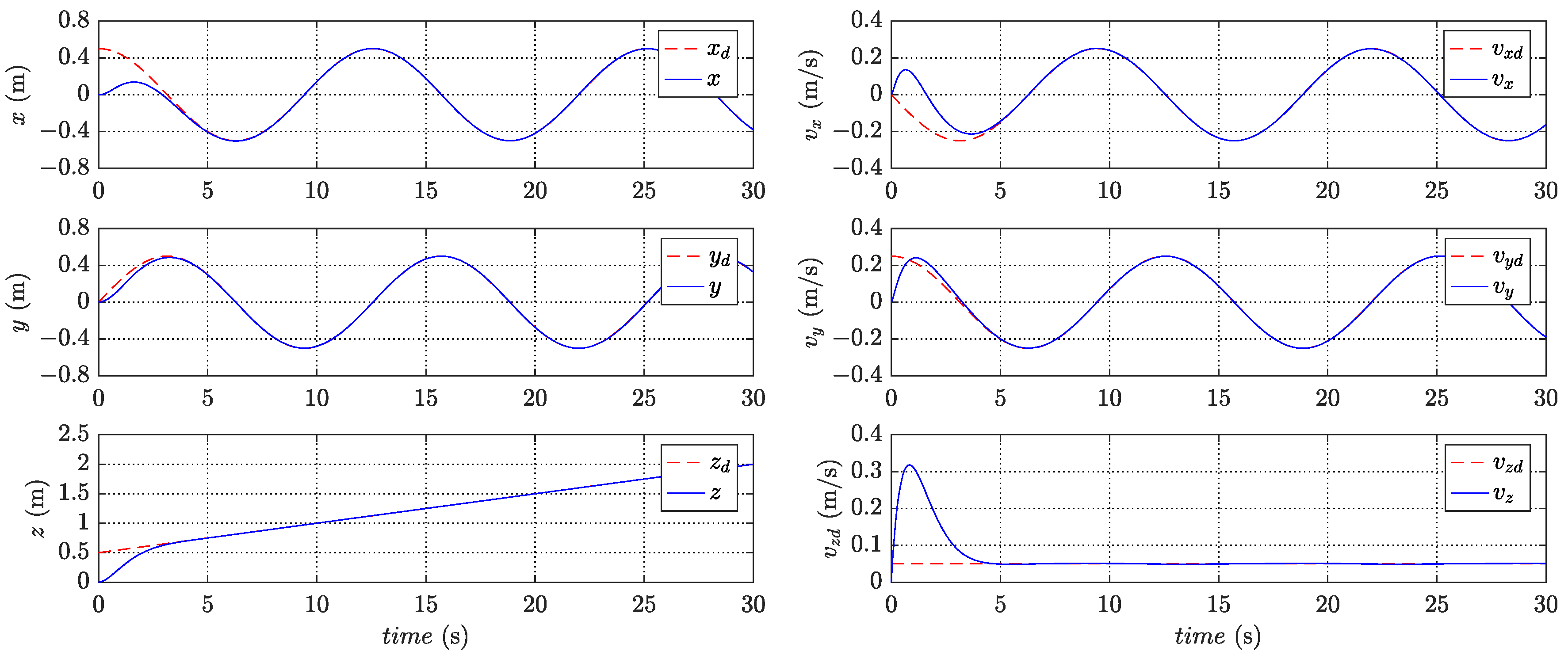
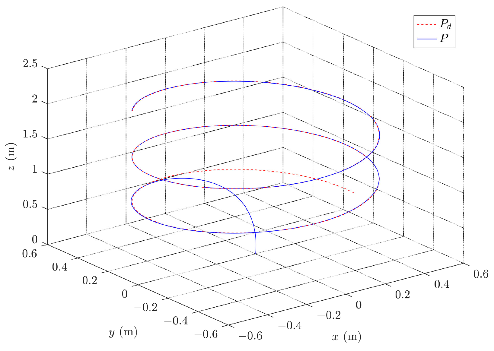
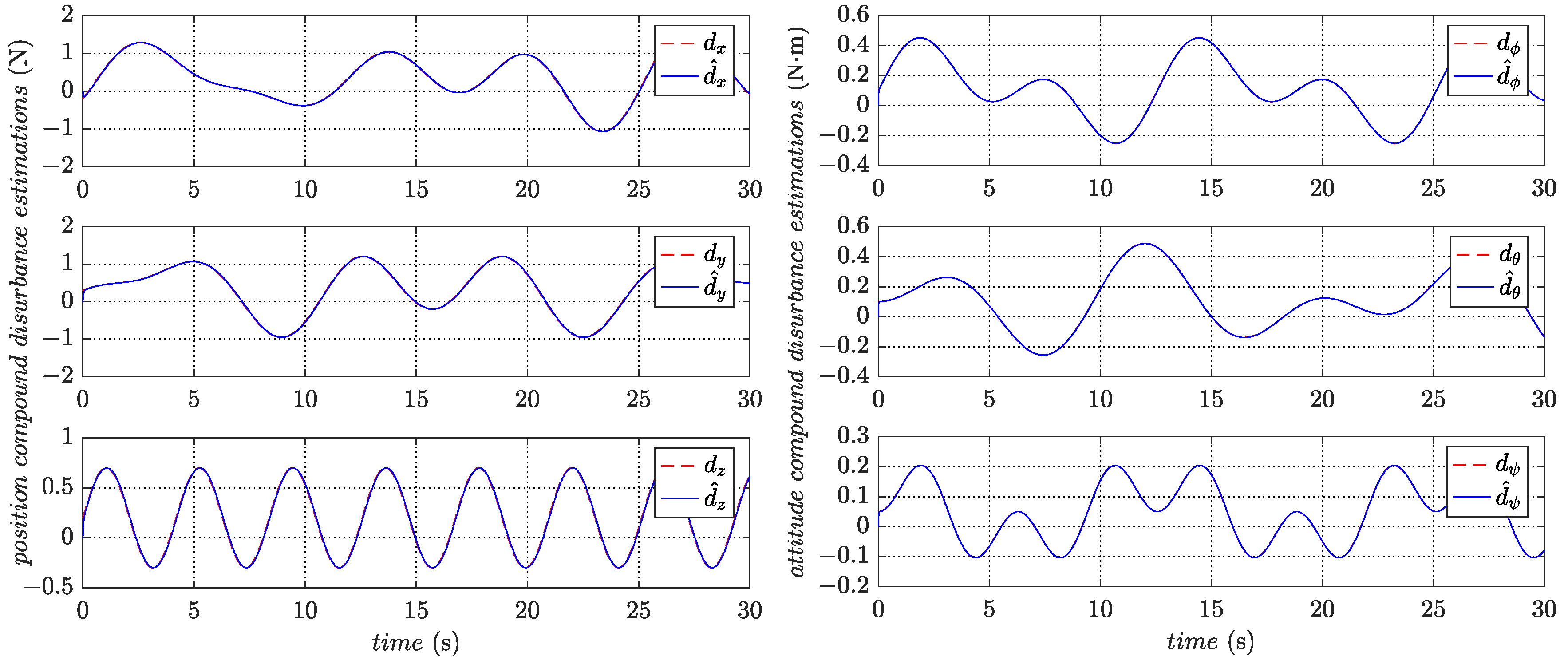
A representative desired trajectory is selected to emulate the trajectory tracking performance of the quadrotor. The desired trajectory is designed as $P_d=[0.5cos(0.5t),0.5sin(0.5t),$${0.05t+0.5]}^{\mathrm{T}}$ and ${\psi }_d=\pi /12$. In addition, referring to [57,58], the unknown compound disturbances considered are described as $d_p={[0.3+0.5(sin(t)+sin(0.5t)-cos(0.8t));0.3+0.5(cos(t)+sin(0.5t)-cos(0.8t));0.2+0.5sin(1.5t)]}^{\mathrm{T}}$ and $d_a=[0.1+0.2(sin(t)+sin(0.5t));$. In this way, the performance of the disturbance observers is reflected by comparing them with the estimates. The initial states of the quadrotor are all set to zero.

The vector-valued functions of the disturbance observers are designed as $p_1(x_1)=l_1(x_1)x_1$, $p_2(x_2)=l_2(x_2)x_2$, while the observer gains are selected as

$$l_1(x_1)=\left[\begin{array}{cccccc}0& 0& 0& 60& 0& 0\\ 0& 0& 0& 0& 60& 0\\ 0& 0& 0& 0& 0& 60\end{array}\right],l_2(x_2)=\left[\begin{array}{cccccc}0& 0& 0& 5& 0& 0\\ 0& 0& 0& 0& 5& 0\\ 0& 0& 0& 0& 0& 5\end{array}\right].$$

Clearly, $l_1(x_1)g_1(x_1)$ and $l_2(x_2)g_2(x_2)$ are positive definite and satisfy the design requirements of Theorem 1. To derive the appropriate dynamic performance, the parameters of the performance index functions are designed as $Q_1=\mathrm{diag}\{7,7,10,9,9,6\}$, $Q_2=\mathrm{diag}\{1.5,1.5,1.2,0.3,0.3,0.4\}$, $R_1=R_2=I_3$. The activation functions are designed as ${\phi }_{c1}(e_1)={[e_x^2,e_x{e}_{v_x},e_y^2,e_y{e}_{v_y},e_z^2,e_z{e}_{v_z},e_{v_x}^2,e_{v_y}^2,e_{v_z}^2]}^{\mathrm{T}}$, ${\phi }_{c2}(e_2)=[e_{\varphi }^2,e_{\varphi }{e}_p,e_{\theta }^2,e_{\theta }{e}_q,e_{\psi }^2,e_{\psi }{e}_r,e_p^2,$$e_p{e}_q,e_p{e}_r,e_q^2,e_q{e}_r,e_r^2,e_{\varphi }^2{e}_q{e}_r,e_{\varphi }{e}_p{e}_q{e}_r,e_{\theta }^2{e}_p{e}_r,e_{\theta }{e}_p{e}_q{e}_r,e_{\psi }^2{e}_p{e}_q,e_{\psi }{e}_p{e}_q{e}_r,e_p^4,e_p^3{e}_q,e_p^3{e}_r,e_p^2{e}_q^2,e_p^2{e}_q{e}_r,$$e_p^2{e}_r^2,e_p{e}_q^3,e_p{e}_q^2{e}_r,e_p{e}_q{e}_r^2,e_p{e}_r^3,e_q^4,e_q^3{e}_r,e_q^2{e}_r^2,e_q{e}_r^3,e_r^4{]}^{\mathrm{T}}$. The relevant constants of the weight update laws are selected as ${\alpha }_{11}=10$, ${\alpha }_{12}=0.01$, ${\alpha }_{13}=0.1$, ${\alpha }_{21}=20$, ${\alpha }_{22}=0.001$, ${\alpha }_{23}=0.1$. The Lyapunov function candidates are selected as $J_1(e_1)=\frac{1}{2}{e}_1^{\mathrm{T}}{e}_1$ and $J_2(e_2)=\frac{1}{2}{e}_2^{\mathrm{T}}{e}_2$. The initial weights are assigned values within the interval $[0,1]$.

The PE condition is ensured by the method mentioned in Remark 5 to excite the system states. The weights gradually vary to become slower and stabilize during the learning process. The converged weights are already very close to the ideal weights after sufficient learning. The convergence of the whole critic network weights ${\widehat{W}}_{c1}$, ${\widehat{W}}_{c2}$ in the learning processes are depicted in Figure 3. The final converged values of ${\widehat{W}}_{c1}$, ${\widehat{W}}_{c2}$ are as follows

$$\begin{array}{cc}\hfill {\widehat{W}}_{c1}=& {[11.3714,9.4718,11.3713,9.4718,13.1589,11.3203,7.6718,7.6718,7.4279]}^{\mathrm{T}},\hfill \\ \hfill {\widehat{W}}_{c2}=& [0.7500,0.0646,0.7182,0.0630,0.8202,0.0888,0.0214,-0.0006,-0.0004,\hfill \\ & 0.0221,-0.0024,0.0287,0.0092,0.0045,0.0346,-0.0059,-0.0096,0.0453,\hfill \\ & 0.0340,0.0211,0.0106,-0.0025,0.0039,-0.0045,0.0227,0.0126,0.0155,\hfill \\ & {0.0076,0.0256,0.0020,0.0016,0.0090,-0.0185]}^{\mathrm{T}}.\hfill \end{array}$$

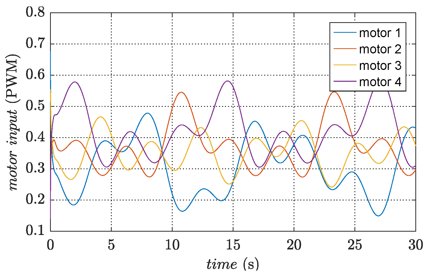
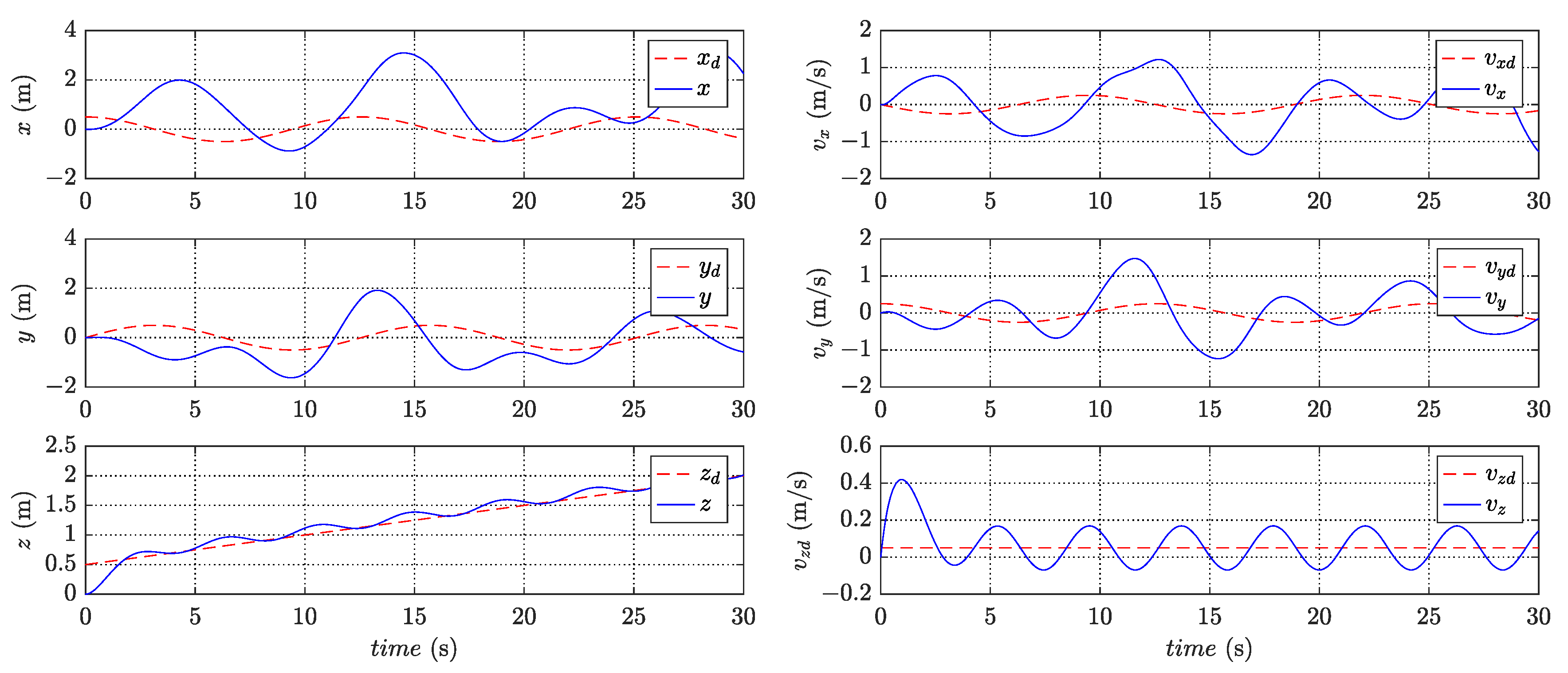
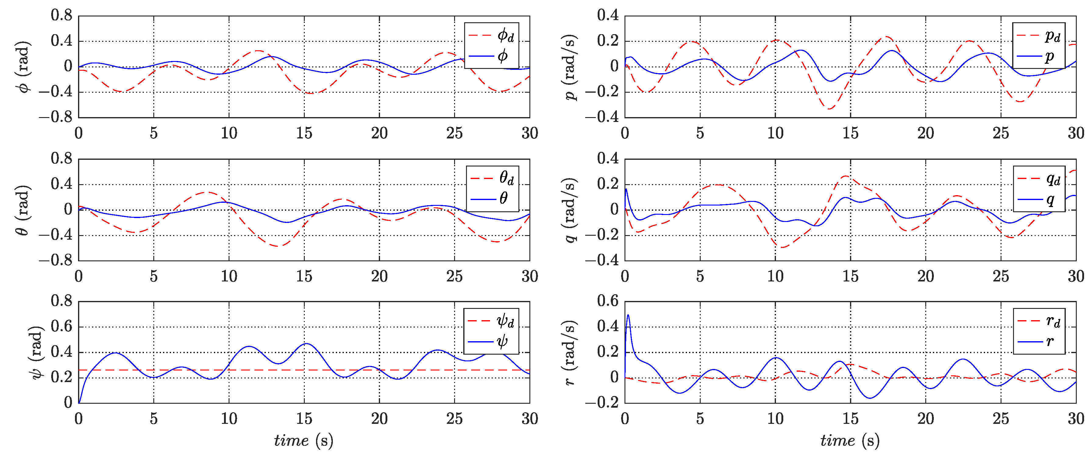
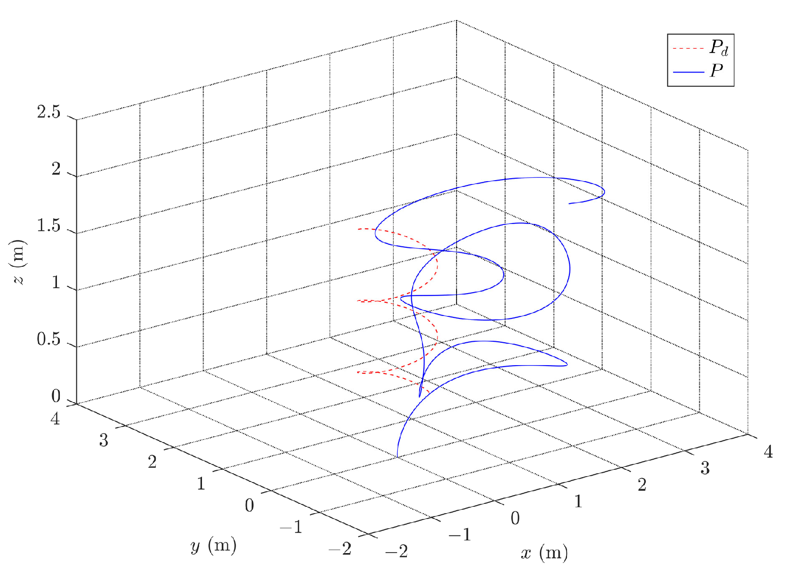
The converged weights are used to design the approximate feedback optimal control inputs. Figure 4 and Figure 5 present the variation of states in trajectory tracking control, revealing the corresponding tracking errors in Figure 6 and Figure 7. In addition, Figure 8 visualizes the path in three-dimensional space, whereas Figure 9 illustrates the PWM signals for the motors. The figures clearly demonstrate that the quadrotor system effectively tracks the desired trajectory and achieves a small convergence bound for the tracking error. These results highlight the rapidity and accuracy of the designed controller in the control process.

The estimates for the compound disturbances are depicted in Figure 10. It shows that the estimated values from the disturbance observers can quickly follow the actual compound disturbances. Moreover, the trajectory tracking control performs well in the presence of compound disturbances, which implies the robustness of the designed controller.

In order to verify that the designed controller rejects the compound disturbances, a comparative simulation is performed without the disturbance observers in the position subsystem and the attitude subsystem. The control inputs use only the control inputs designed for the nominal system. Under such control, the variation of states is presented in Figure 11 and Figure 12, while Figure 13 and Figure 14 show the corresponding tracking errors.

By comparing the simulation results, it is clear that the trajectory tracking control of the quadrotor cannot be realized without the robust compensation inputs. Thus, further demonstrating the robustness of the designed controller. Moreover, the corresponding path in three-dimensional space and the PWM signals of the motors are shown in Figure 15 and Figure 16, respectively.

In summary, the controller designed for quadrotor trajectory tracking control has good dynamic performance, high tracking accuracy and strong robustness when the quadrotor is subjected to compound disturbances.

6. Conclusions

This paper proposes a robust approximate optimal controller for the trajectory tracking control of the quadrotor with unknown compound disturbances. By incorporating the estimated values of compound disturbances that are estimated by the disturbance observers into the control design, the effect of compound disturbances can be suppressed, resulting in ensured tracking accuracy and improved robustness. Moreover, the ADP method can then be utilized in the nominal system for ensuring the performance index of the control. The stability of the closed-loop system is analyzed by the Lyapunov theorem, which demonstrates that the tracking errors are UUB. Simulation results further confirm the robustness and effectiveness of the designed controller. In future work, experiments will be considered to validate the performance of the proposed controller.

References

1. Hassanalian, M.; Abdelkefi, A. Classifications, applications, and design challenges of drones: A review. Prog. Aerosp. Sci. 2017, 91, 99–131. [Google Scholar] [CrossRef]
2. Salem, K.A.; Palaia, G.; Chiarelli, M.R.; Bianchi, M. A simulation framework for aircraft take-off considering ground effect aerodynamics in conceptual design. Aerospace 2023, 10, 459. [Google Scholar] [CrossRef]
3. Salem, K.A.; Palaia, G.; Quarta, A.A. Review of hybrid-electric aircraft technologies and designs: Critical analysis and novel solutions. Prog. Aerosp. Sci. 2023, 141, 100924. [Google Scholar] [CrossRef]
4. Shao, S.; Chen, M.; Hou, J.; Zhao, Q. Event-triggered-based discrete-time neural control for a quadrotor UAV using disturbance observer. IEEE/ASME Trans. Mechatronics 2021, 26, 689–699. [Google Scholar] [CrossRef]
5. Idrissi, M.; Salami, M.; Annaz, F. A review of quadrotor unmanned aerial vehicles: Applications, architectural design and control algorithms. J. Intell. Robot. Syst. 2022, 104, 22. [Google Scholar] [CrossRef]
6. Rinaldi, F.; Chiesa, S.; Quagliotti, F. Linear quadratic control for quadrotors UVAs dynamics and formation flight. J. Intell. Robot. Syst. 2013, 70, 203–220. [Google Scholar] [CrossRef]
7. Dharmawan, A.; Priyambodo, T.K. Model of linear quadratic regulator (lqr) control method in hovering state of quadrotor. J. Telecommun. Electron. Comput. Eng. (JTEC) 2017, 9, 135–143. [Google Scholar]
8. Alonge, F.; D’Ippolito, F.; Fagiolini, A.; Garraffa, G.; Sferlazza, A. Trajectory robust control of autonomous quadcopters based on model decoupling and disturbance estimation. Int. J. Adv. Robot. Syst. 2021, 18, 1729881421996974. [Google Scholar] [CrossRef]
9. Yang, Y.; Yan, Y. Attitude regulation for unmanned quadrotors using adaptive fuzzy gain-scheduling sliding mode control. Aerosp. Sci. Technol. 2016, 54, 208–217. [Google Scholar] [CrossRef]
10. Avram, R.C.; Zhang, X.; Muse, J. Nonlinear adaptive fault-tolerant quadrotor altitude and attitude tracking with multiple actuator faults. IEEE Trans. Control. Syst. Technol. 2017, 26, 701–707. [Google Scholar] [CrossRef]
11. Chen, F.; Lei, W.; Zhang, K.; Tao, G.; Jiang, B. A novel nonlinear resilient control for a quadrotor UVA via backstepping control and nonlinear disturbance observer. Nonlinear Dyn. 2016, 85, 1281–1295. [Google Scholar] [CrossRef]
12. Liu, H.; Xi, J.; Zhong, Y. Robust attitude stabilization for nonlinear quadrotor systems with uncertainties and delays. IEEE Trans. Ind. Electron. 2017, 64, 5585–5594. [Google Scholar] [CrossRef]
13. Liu, E.; Yan, Y.; Yang, Y. Neural network approximation-based backstepping sliding mode control for spacecraft with input saturation and dynamics uncertainty. Acta Astronaut. 2022, 191, 1–10. [Google Scholar] [CrossRef]
14. Li, R.; Chen, M.; Wu, Q. Robust control for an unmanned helicopter with constrained flapping dynamics. Chin. J. Aeronaut. 2018, 31, 2136–2148. [Google Scholar] [CrossRef]
15. Li, R.; Chen, M.; Wu, Q. Adaptive neural tracking control for uncertain nonlinear systems with input and output constraints using disturbance observer. Neurocomputing 2017, 235, 27–37. [Google Scholar] [CrossRef]
16. Yang, Y.; Modares, H.; Vamvoudakis, K.G.; He, W.; Xu, C.Z.; Wunsch, D.C. Hamiltonian-driven adaptive dynamic programming with approximation errors. IEEE Trans. Cybern. 2021, 52, 13762–13773. [Google Scholar] [CrossRef]
17. Xue, S.; Luo, B.; Liu, D. Event-triggered adaptive dynamic programming for zero-sum game of partially unknown continuous-time nonlinear systems. IEEE Trans. Syst. Man Cybern. Syst. 2018, 50, 3189–3199. [Google Scholar] [CrossRef]
18. Du, Y.; Jiang, B.; Ma, Y.; Cheng, Y. Robust ADP-based sliding-mode fault-tolerant control for nonlinear systems with application to spacecraft. Appl. Sci. 2022, 12, 1673. [Google Scholar] [CrossRef]
19. Huang, Y.; Wang, D.; Liu, D. Bounded robust control design for uncertain nonlinear systems using single-network adaptive dynamic programming. Neurocomputing 2017, 266, 128–140. [Google Scholar] [CrossRef]
20. Wang, D.; Liu, D.; Li, H. Policy iteration algorithm for online design of robust control for a class of continuous-time nonlinear systems. IEEE Trans. Autom. Sci. Eng. 2014, 11, 627–632. [Google Scholar] [CrossRef]
21. Dou, L.; Su, X.; Zhao, X.; Zong, Q.; He, L. Robust tracking control of quadrotor via on-policy adaptive dynamic programming. Int. J. Robust Nonlinear Control 2021, 31, 2509–2525. [Google Scholar] [CrossRef]
22. Mu, C.; Zhang, Y. Learning-based robust tracking control of quadrotor with time-varying and coupling uncertainties. IEEE Trans. Neural Netw. Learn. Syst. 2019, 31, 259–273. [Google Scholar] [CrossRef]
23. Chen, W.H.; Yang, J.; Guo, L.; Li, S. Disturbance-observer-based control and related methods—An overview. IEEE Trans. Ind. Electron. 2015, 63, 1083–1095. [Google Scholar] [CrossRef]
24. Chen, M.; Xiong, S.; Wu, Q. Tracking flight control of quadrotor based on disturbance observer. IEEE Trans. Syst. Man Cybern. Syst. 2019, 51, 1414–1423. [Google Scholar] [CrossRef]
25. Chen, F.; Jiang, R.; Zhang, K.; Jiang, B.; Tao, G. Robust backstepping sliding-mode control and observer-based fault estimation for a quadrotor UVA. IEEE Trans. Ind. Electron. 2016, 63, 5044–5056. [Google Scholar]
26. Shao, X.; Liu, J.; Cao, H.; Shen, C.; Wang, H. Robust dynamic surface trajectory tracking control for a quadrotor UVA via extended state observer. Int. J. Robust Nonlinear Control 2018, 28, 2700–2719. [Google Scholar] [CrossRef]
27. Mofid, O.; Mobayen, S. Adaptive sliding mode control for finite-time stability of quad-rotor UAVs with parametric uncertainties. ISA Trans. 2018, 72, 1–14. [Google Scholar] [CrossRef] [PubMed]
28. Lei, W.; Li, C.; Chen, M.Z. Robust adaptive tracking control for quadrotors by combining PI and self-tuning regulator. IEEE Trans. Control Syst. Technol. 2018, 27, 2663–2671. [Google Scholar] [CrossRef]
29. Maqsood, H.; Qu, Y. Nonlinear disturbance observer based sliding mode control of quadrotor helicopter. J. Electr. Eng. Technol. 2020, 15, 1453–1461. [Google Scholar] [CrossRef]
30. Hua, H.; Fang, Y.; Zhang, X.; Lu, B. A novel robust observer-based nonlinear trajectory tracking control strategy for quadrotors. IEEE Trans. Control Syst. Technol. 2020, 29, 1952–1963. [Google Scholar] [CrossRef]
31. Song, R.; Lewis, F.L. Robust optimal control for a class of nonlinear systems with unknown disturbances based on disturbance observer and policy iteration. Neurocomputing 2020, 390, 185–195. [Google Scholar] [CrossRef]
32. Lee, D. Nonlinear disturbance observer-based robust control for spacecraft formation flying. Aerosp. Sci. Technol. 2018, 76, 82–90. [Google Scholar] [CrossRef]
33. Yuan, W.; Gao, G. Sliding mode control of the automobile electro-coating conveying mechanism with a nonlinear disturbance observer. Adv. Mech. Eng. 2018, 10, 1687814018795748. [Google Scholar] [CrossRef]
34. Orozco Soto, S.M.; Cacace, J.; Ruggiero, F.; Lippiello, V. Active Disturbance Rejection Control for the Robust Flight of a Passively Tilted Hexarotor. Drones 2022, 6, 258. [Google Scholar] [CrossRef]
35. Wang, Y.; Sun, J.; He, H.; Sun, C. Deterministic policy gradient with integral compensator for robust quadrotor control. IEEE Trans. Syst. Man Cybern. Syst. 2019, 50, 3713–3725. [Google Scholar] [CrossRef]
36. Li, C.; Wang, Y.; Yang, X. Adaptive fuzzy control of a quadrotor using disturbance observer. Aerosp. Sci. Technol. 2022, 128, 107784. [Google Scholar] [CrossRef]
37. Fan, Y.; Guo, H.; Han, X.; Chen, X. Research and verification of trajectory tracking control of a quadrotor carrying a load. Appl. Sci. 2022, 12, 1036. [Google Scholar] [CrossRef]
38. Wang, B.; Yu, X.; Mu, L.; Zhang, Y. Disturbance observer-based adaptive fault-tolerant control for a quadrotor helicopter subject to parametric uncertainties and external disturbances. Mech. Syst. Signal Process. 2019, 120, 727–743. [Google Scholar] [CrossRef]
39. Fei, Y.; Shi, P.; Lim, C.C. Robust and collision-free formation control of multiagent systems with limited information. IEEE Trans. Neural Netw. Learn. Syst. 2021, 34, 4286–4295. [Google Scholar] [CrossRef]
40. Fei, Y.; Shi, P.; Lim, C.C. Robust formation control for multi-agent systems: A reference correction based approach. IEEE Trans. Circuits Syst. Regul. Pap. 2021, 68, 2616–2625. [Google Scholar] [CrossRef]
41. Xia, R.; Wu, Q.; Shao, S. Disturbance observer-based optimal flight control of near space vehicle with external disturbance. Trans. Inst. Meas. Control 2020, 42, 272–284. [Google Scholar] [CrossRef]
42. Sun, J.; Liu, C. Disturbance observer-based robust missile autopilot design with full-state constraints via adaptive dynamic programming. J. Frankl. Inst. 2018, 355, 2344–2368. [Google Scholar] [CrossRef]
43. Zhang, H.; Cui, L.; Zhang, X.; Luo, Y. Data-driven robust approximate optimal tracking control for unknown general nonlinear systems using adaptive dynamic programming method. IEEE Trans. Neural Netw. 2011, 22, 2226–2236. [Google Scholar] [CrossRef] [PubMed]
44. Xu, N.; Niu, B.; Wang, H.; Huo, X.; Zhao, X. Single-network ADP for solving optimal event-triggered tracking control problem of completely unknown nonlinear systems. Int. J. Intell. Syst. 2021, 36, 4795–4815. [Google Scholar] [CrossRef]
45. Xia, R.; Wu, Q.; Chen, M. Disturbance observer-based optimal longitudinal trajectory control of near space vehicle. Sci. China Inf. Sci. 2019, 62, 1–3. [Google Scholar] [CrossRef]
46. Sun, J.; Liu, C. Backstepping-based adaptive dynamic programming for missile-target guidance systems with state and input constraints. J. Frankl. Inst. 2018, 355, 8412–8440. [Google Scholar] [CrossRef]
47. Wang, D.; Liu, D.; Li, H.; Ma, H. Neural-network-based robust optimal control design for a class of uncertain nonlinear systems via adaptive dynamic programming. Inf. Sci. 2014, 282, 167–179. [Google Scholar] [CrossRef]
48. Zheng, S.; Shi, P.; Wang, S.; Shi, Y. Adaptive neural control for a class of nonlinear multiagent systems. IEEE Trans. Neural Netw. Learn. Syst. 2020, 32, 763–776. [Google Scholar] [CrossRef] [PubMed]
49. Fan, Q.Y.; Yang, G.H. Adaptive actor–critic design-based integral sliding-mode control for partially unknown nonlinear systems with input disturbances. IEEE Trans. Neural Netw. Learn. Syst. 2015, 27, 165–177. [Google Scholar] [CrossRef] [PubMed]
50. Vamvoudakis, K.G.; Lewis, F.L. Online actor–critic algorithm to solve the continuous-time infinite horizon optimal control problem. Automatica 2010, 46, 878–888. [Google Scholar] [CrossRef]
51. Liu, D.; Xue, S.; Zhao, B.; Luo, B.; Wei, Q. Adaptive dynamic programming for control: A survey and recent advances. IEEE Trans. Syst. Man Cybern. Syst. 2020, 51, 142–160. [Google Scholar] [CrossRef]
52. Zhao, B.; Liu, D.; Luo, C. Reinforcement learning-based optimal stabilization for unknown nonlinear systems subject to inputs with uncertain constraints. IEEE Trans. Neural Netw. Learn. Syst. 2019, 31, 4330–4340. [Google Scholar] [CrossRef] [PubMed]
53. Wang, D.; Liu, D.; Zhang, Y.; Li, H. Neural network robust tracking control with adaptive critic framework for uncertain nonlinear systems. Neural Netw. 2018, 97, 11–18. [Google Scholar] [CrossRef] [PubMed]
54. Liu, D.; Wei, Q.; Wang, D.; Yang, X.; Li, H. Adaptive Dynamic Programming with Applications in Optimal Control; Springer International Publishing: Berlin/Heidelberg, Germany, 2017. [Google Scholar]
55. Lewis, F.L.; Jagannathan, S.; Yesildirek, A. Neural Network Control of Robot Manipulators and Nonlinear Systems; Taylor & Francis: London, UK, 1999. [Google Scholar]
56. Castillo, A.; Sanz, R.; Garcia, P.; Qiu, W.; Wang, H.; Xu, C. Disturbance observer-based quadrotor attitude tracking control for aggressive maneuvers. Control Eng. Pract. 2019, 82, 14–23. [Google Scholar] [CrossRef]
57. Mobayen, S.; El-Sousy, F.F.; Alattas, K.A.; Mofid, O.; Fekih, A.; Rojsiraphisal, T. Adaptive fast-reaching nonsingular terminal sliding mode tracking control for quadrotor UAVs subject to model uncertainties and external disturbances. Ain Shams Eng. J. 2023, 14, 102059. [Google Scholar] [CrossRef]
58. Shao, X.; Yue, X.; Li, J. Event-triggered robust control for quadrotors with preassigned time performance constraints. Appl. Math. Comput. 2021, 14, 102059. [Google Scholar] [CrossRef]
Figure 1. Basic structure of the quadrotor.
Aerospace 11 00149 g001
Figure 2. Control design of the quadrotor.
Aerospace 11 00149 g002
Figure 3. Convergence of critic network weights.
Aerospace 11 00149 g003
Figure 4. Variation of states in the position subsystem.
Aerospace 11 00149 g004
Figure 5. Variation of states in the attitude subsystem.
Aerospace 11 00149 g005
Figure 6. Tracking errors in the position subsystem.
Aerospace 11 00149 g006
Figure 7. Tracking errors in the attitude subsystem.
Aerospace 11 00149 g007
Figure 8. Results of three-dimensional path.
Aerospace 11 00149 g008
Figure 9. Pulse-width of input signals.
Aerospace 11 00149 g009
Figure 10. Estimates of compound disturbances.
Aerospace 11 00149 g010
Figure 11. Variation of states in the position subsystem without disturbance observers.
Aerospace 11 00149 g011
Figure 12. Variation of states in the attitude subsystem without disturbance observers.
Aerospace 11 00149 g012
Figure 13. Tracking errors in the position subsystem without disturbance observers.
Aerospace 11 00149 g013
Figure 14. Tracking errors in the attitude subsystem without disturbance observers.
Aerospace 11 00149 g014
Figure 15. Results of three-dimensional path without disturbance observers.
Aerospace 11 00149 g015
Figure 16. Pulse-width of input signals without disturbance observers.
Aerospace 11 00149 g016