RBFNN-Based Anti-Input Saturation Control for Hypersonic Vehicles

Abstract

In hypersonic flight control, characterized by challenges posed by input saturation, model parameter uncertainties, and external disturbances, this paper introduces a pioneering anti-input saturation control method based on RBFNN adaptivity. We have developed adaptive laws to enhance control system adaptability and robustness by integrating mission profiles, actuator saturation failure modes, and self-evolving neural network design. Furthermore, our approach introduces a novel anti-input saturation auxiliary system, effectively addressing input saturation constraints. This innovation ensures system stability and precise tracking, even in severe input saturation constraints. The results reveal that the system’s steady-state tracking error remains under 2% under input saturation constraints, and the convergence speed demonstrates an impressive 20% improvement. These findings underscore this research’s substantial advancement in hypersonic flight control. It may significantly enhance the controllability and performance of hypersonic vehicles in real-world scenarios.

1. Introduction

Hypersonic aircraft have captured substantial interest and fascination in recent years, primarily due to their astounding capabilities, encompassing unparalleled penetration potential and extraordinary destructive effects. Compared to traditional aircraft, hypersonic aircraft possess inherent traits that set them apart, including nonlinearity, rapidly changing dynamics, and strong coupling [1,2,3]. These distinctive characteristics bring about intricate challenges, further exacerbated by significant model uncertainty, when designing control systems for hypersonic aircraft. The complexities associated with hypersonic flight are multifaceted and substantial. They arise from the intricate interplay of various factors, making crafting effective control systems for these aircraft arduous. These factors include the unique qualities intrinsic to hypersonic aviation, such as their nonlinearity, rapid and time-varying dynamics, and strong coupling, necessitating innovative solutions to address and manage these complexities. The substantial model uncertainty further complicates the formidable challenges in developing robust and efficient control systems tailored for hypersonic aircraft.

The attention and interest in hypersonic aircraft stem from their distinctive and exceptional capabilities, particularly their ability to penetrate and cause substantial damage. However, these extraordinary capabilities also come with intricacies and challenges that must be overcome, requiring innovative and advanced solutions in control system design. In the intricate and demanding flight environments hypersonic aircraft navigate, unpredictable airflow disturbances introduce a critical challenge, leading to actuator saturation. This undesirable condition significantly hampers the effectiveness of control inputs, impairing the aircraft’s maneuverability and responsiveness [4,5]. The limitations imposed on the actuators result in a constrained control force, which, in turn, has adverse effects on the aircraft’s overall flight performance.

Moreover, this limitation on control inputs can even escalate to inducing instability within the aircraft’s control system, further underscoring the importance of addressing and mitigating input saturation concerns. Conversely, another aspect that exacerbates the complexity of managing hypersonic flight is the issue of operating at excessively high fuel equivalence ratios. Such a condition can provoke engine thermal blockage. When the actuator and fuel equivalence ratio of the aircraft reaches a certain upper or lower limit of the input signal, the saturation phenomenon occurs, leading to negative effects on the system response, which has the potential to pose grave risks and challenges to the aircraft’s operation [6,7]. This further emphasizes the critical need to address and alleviate the issues associated with input saturation. The actuator saturation and engine thermal blockage present a complex set of constraints that require innovative solutions to ensure hypersonic aircraft safety, stability, and optimal performance in these demanding flight conditions.

Prior research has made notable strides in addressing actuator constraints and dynamics issues, using auxiliary systems to counteract saturation nonlinearity in control commands, and employing neural adaptive mechanisms to mitigate uncertainties and disturbances [8]. Additional contributions have explored auxiliary systems generating compensation signals to manage actuator amplitude constraints [9], introduced anti-saturation fixed-time compensators to ensure system stability and expedite exit from saturation regions [10,11], and proposed Nussbaum gain adaptive controllers to address actuator saturation during hypersonic aircraft re-entry [12]. Fuzzy methods have also been used to construct auxiliary systems with adaptive laws for fuzzy interference attenuators [13], and adaptive fault-tolerant controllers based on obstacle Lyapunov functions have been designed to resolve input saturation issues [14]. Furthermore, adaptive neural control with auxiliary error compensation has been employed to effectively follow speed and altitude commands in actuator saturation system uncertainty [15].

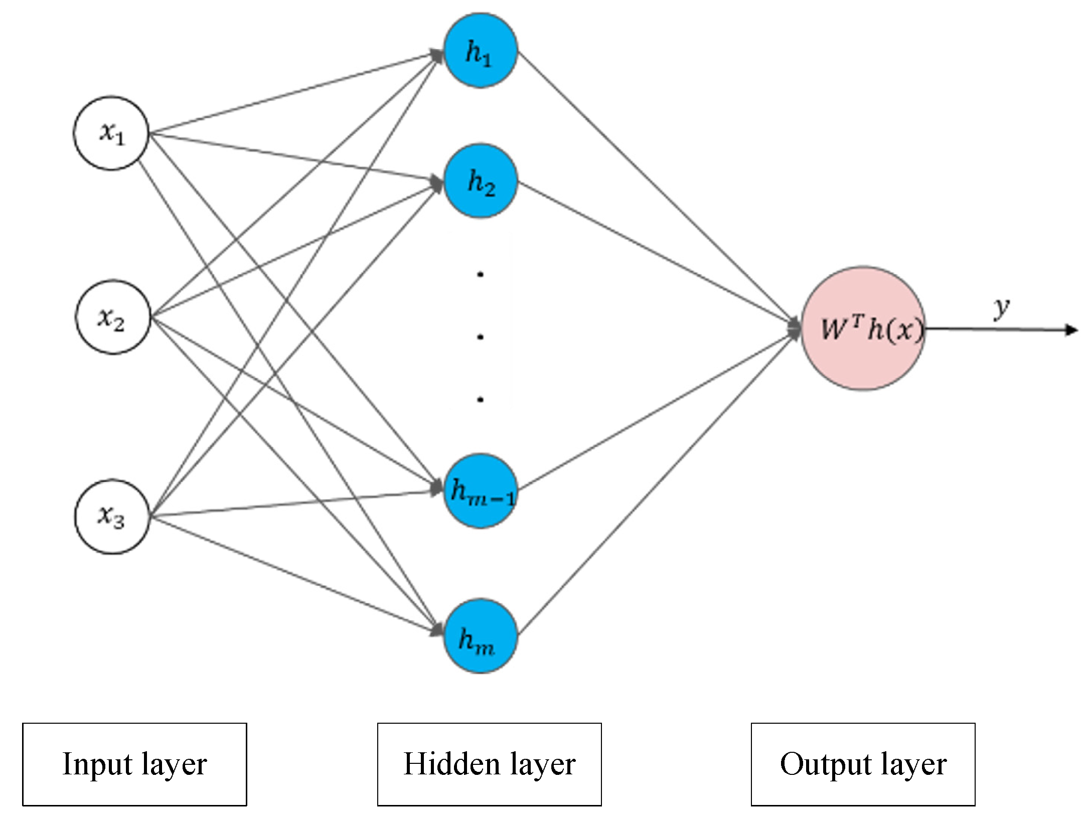
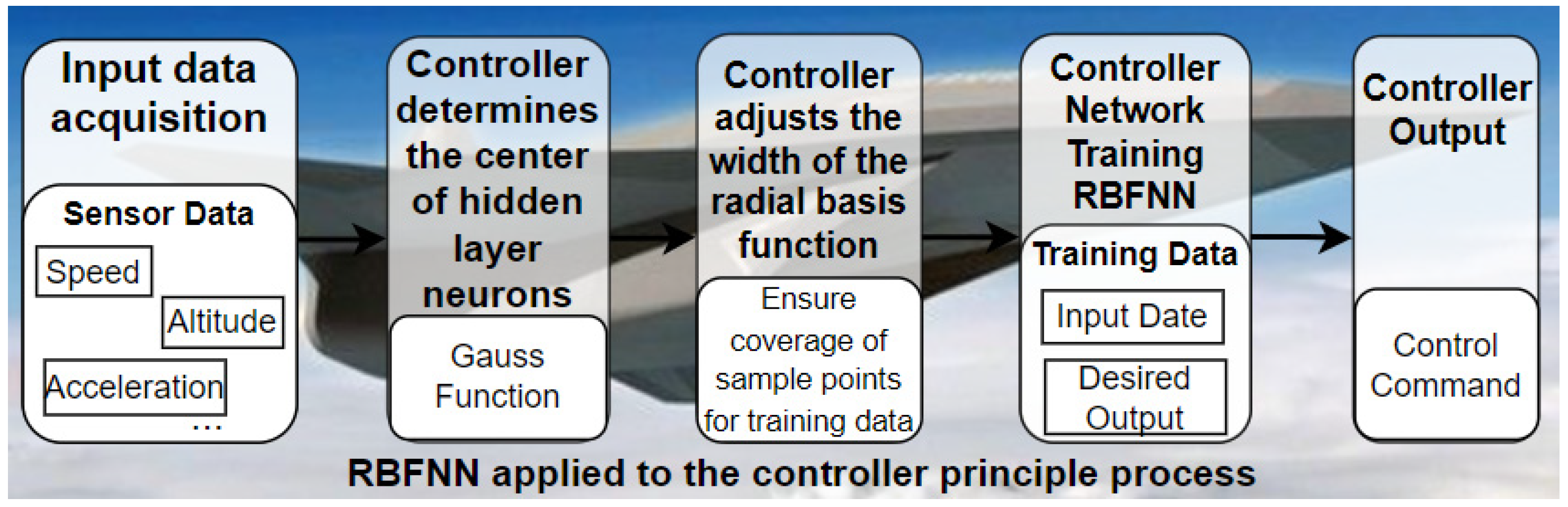
While significant progress has been made in the field, it is essential to recognize that persistent challenges remain, particularly in actuator saturation under high dynamic conditions, signal noise identification, and developing anti-saturation strategies that can adapt with precision in real time. This article takes a pioneering approach to address these gaps in current research by integrating two distinct yet complementary domains: Radial Basis Function Neural Network (RBFNN) theory and adaptive control theory. This integration is thoughtfully tailored to hypersonic vehicles’ mission profiles and operational environments. The outcome of this novel fusion is the development of an RBFNN adaptive controller and an anti-saturation auxiliary system. The RBFNN adaptive controller is meticulously designed to enhance system stability and ensure precise tracking, even in severe input saturation scenarios. Leveraging the capabilities of neural networks, this controller adapts and optimizes control inputs, effectively mitigating the adverse effects of actuator saturation in high dynamic conditions. Its ability to adapt to changing needs and maintain precise control addresses a long-standing challenge in hypersonic flight control. In parallel, the anti-saturation auxiliary system is engineered to work harmoniously with the RBFNN adaptive controller. This auxiliary system can dynamically adjust the precision of anti-saturation measures, offering a responsive and timely approach to counteract actuator saturation. This adaptability is designed to cater to hypersonic flight’s unique and demanding needs, where input saturation levels can fluctuate rapidly due to varying mission profiles and operational environments. By uniting the strengths of RBFNN and adaptive control theory and applying them within the context of hypersonic vehicles, this article strives to bridge existing research gaps and advance the boundaries of control systems. The ultimate objective is to establish more excellent system stability and precision in tracking, even in the face of challenging and dynamically changing conditions, thus making a substantial contribution to the advancement of hypersonic aircraft technology.

The goal is to address the complex challenges of hypersonic flight control, which are characterized by input saturation, model uncertainty, and external disturbances. Due to the inherent characteristics of hypersonic aircraft, including nonlinearity, rapidly changing dynamics, and strong coupling, these challenges are particularly evident. This research introduces several pivotal innovations that significantly advance the field. To enhance the adaptability and robustness of the control system, we have developed adaptive laws integrating mission profiles, actuator saturation failure modes, and a self-evolving neural network design. In the meantime, the approach introduces a novel anti-input saturation auxiliary system, addressing input saturation constraints and ensuring system stability and precise tracking even in severe conditions. First, the RBFNN adaptive controller stands out with its enhanced capabilities regarding system state convergence and tracking accuracy compared to previous methodologies [16]. It substantially improves system state convergence, ensuring the aircraft’s operations are more efficient and safer.

Additionally, this advanced controller achieves superior tracking accuracy, which is paramount in guiding hypersonic aircraft with precision. Second, this research brings forth a breakthrough in ensuring robust stability even under conditions of severe input saturation, a common challenge in hypersonic flight. The newly developed auxiliary system plays a central role in this achievement, guaranteeing system stability even when confronted with extreme input saturation scenarios during hypersonic flight. This accomplishment enhances hypersonic aircraft’s safety and reliability by ensuring the control system remains effective and precise, even under the most demanding operational conditions. Collectively, these innovations represent a significant leap forward in hypersonic aircraft control, addressing critical issues and advancing state-of-the-art technology.

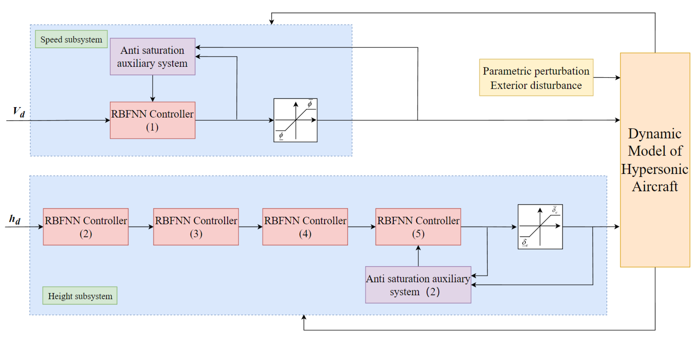
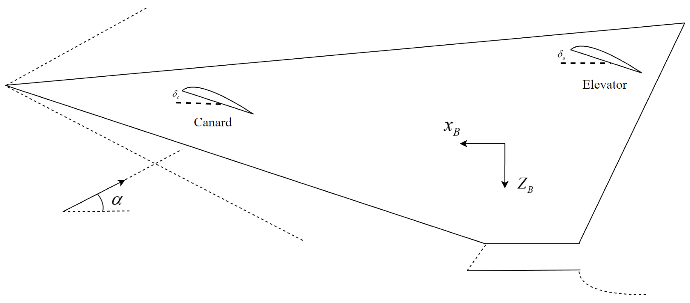
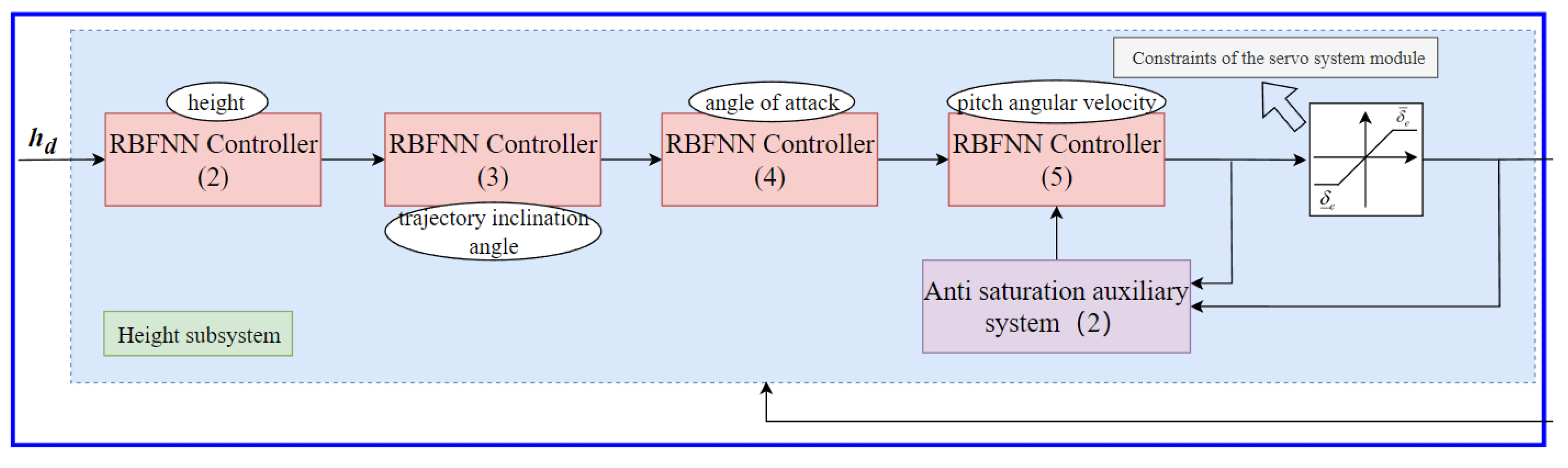
This article commences by transforming the dynamic model of hypersonic aircraft into a strict feedback form, facilitating subsequent controller design. Subsequently, RBFNN adaptive controllers are designed for the speed and height subsystems to address parameter uncertainty effectively. Adaptive laws are introduced upon Lyapunov’s theory, and a novel saturation auxiliary system is devised to manage input constraints. The ensuing stability analysis, grounded in Lyapunov theory, substantiates the efficacy and advancement of the proposed method through comprehensive simulation analysis.

The combination of RBFNN adaptive control and anti-saturation strategies in this research marks a groundbreaking step towards improving hypersonic aircraft’s controllability, stability, and overall robustness. This work represents a significant advancement in state-of-the-art hypersonic vehicle control, offering concrete solutions to the intricate challenges that have historically hindered the realization of their full potential. By integrating cutting-edge neural network techniques with innovative anti-saturation strategies, this research not only pushes the boundaries of what is achievable but also provides practical solutions for enhancing the capabilities of hypersonic aircraft. As a result, it holds the promise of safer and more effective hypersonic missions and opens new horizons for fully utilizing the extraordinary potential of these aircraft.

2. Materials and Methods

2.1. Control Model and Theoretical Basis

2.1.1. Control Model

This article centers on the configuration of the US X-43A. Figure 1 illustrates the longitudinal geometric layout of the X-43A. The aircraft embraces an integrated body/engine design, with

Table 1. Structure parameters.

Geometrical Parameters	Parameter Values
Quality (m)	4378 kg
Moment of inertia (Iyy)	6.770 × 105 kg.m2

presenting the specific geometric parameters. In this particular configuration, the integrated fuselage/engine design offers a notably larger lift-to-drag ratio compared to conventional aircraft. However, this design choice also introduces a substantial coupling of aerodynamics and thrust, thereby presenting considerable challenges in terms of modeling and control.

This article adopts the Lisa model [17], which simplifies the dynamic model of an elastic hypersonic aircraft. The Lisa model considers the elastic effect and includes the elastic state of the hypersonic aircraft in the force and torque. Therefore, the model can accurately reflect the rigid/elastic coupling characteristics. Moreover, in Lisa’s model, canards are incorporated to mitigate the interference of elevators and address the issue of minimum phase influence. Taking the longitudinal channel of a hypersonic aircraft as an example to illustrate the design process of the controller [18], the dynamic model is

$$\{\begin{array}{l}\dot{V}=\frac{T\cos \alpha -D}{m}-g\sin \gamma \\ \dot{h}=V\sin \gamma \\ \dot{\gamma }=\frac{T\sin \alpha +L}{mV}-\frac{g\cos \gamma }{V}\\ \dot{\alpha }=Q-\dot{\gamma }\\ \dot{Q}=M_{yy}/I_{yy}\\ \ddot{\eta }=-2{\zeta }_i{\omega }_i{\dot{\eta }}_i-{\omega }_i^2{\eta }_i+N_i\begin{array}{cc},& (i=1,2,3)\end{array}\end{array}$$

(1)

In the above equation, $V,h,\gamma ,\alpha ,Q$, respectively, represent flight speed, flight altitude, trajectory inclination, angle of attack, and pitch angular velocity; $m$ represents the mass of the aircraft, $g$ represents the Gravitational acceleration, and $I_{yy}$ represents the moment of inertia. The six elastic states are $\{{\eta }_1,{\dot{\eta }}_1,{\eta }_2,{\dot{\eta }}_2,{\eta }_3,{\dot{\eta }}_3\}$; $T,D,L,M_{yy}$ representing thrust, aerodynamic drag, lift, and pitch moment, respectively, and the calculation formula is as follows:

$$\{\begin{array}{l}T=qS(C_{T,\varphi }(\alpha )\varphi +C_T(\alpha )+C_T^{\eta }\eta )\\ C_{T,\varphi }(\alpha )=C_{T,\varphi }^{{\alpha }^3}{\alpha }^3+C_{T,\varphi }^{{\alpha }^2}{\alpha }^2+C_{T,\varphi }^{\alpha }\alpha +C_{T,\varphi }^0\\ C_T(\alpha )=C_T^{{\alpha }^3}{\alpha }^3+C_T^{{\alpha }^2}{\alpha }^2+C_T^{\alpha }\alpha +C_T^0\\ D=qS(C_D^{{\alpha }^2}{\alpha }^2+C_D^{\alpha }\alpha +C_D^0+C_D^{\eta }\eta )\\ L=qS(C_L^{\alpha }\alpha +C_L^0+C_L^{\eta }\eta )\\ M_{yy}=z_{T}T+q\overline{c}S(C_M^{{\alpha }^2}{\alpha }^2+C_M^{\alpha }\alpha +C_M^0+c_e{\delta }_e+C_M^{\eta }\eta )\\ N_i=qS(N_i^{{\alpha }^2}{\alpha }^2+N_i^{\alpha }\alpha +N_i^{{\delta }_e}{\delta }_e+N_i^0+N_i^{\eta }\eta )\end{array}$$

where $q$ is the dynamic pressure, the calculation formula is $q=0.5\rho V^2$; where $\rho$ is the density of air, $S$ is the aircraft reference area (maximum cross section), $\varphi$ is the fuel equivalent ratio, and ${\delta }_e$ is the elevator deflection angle; $C_i^{(·)}$ is a pneumatic parameter [17], $N_i$ is a generalized force. The range of model parameters is shown in

Table 2. The range of model parameters.

Parameters	Lower Limit	Upper Limit
V	7500 ft/s	11,000 ft/s
h	85,000 ft	88,000 ft
γ	−1°	1°
$\alpha$	−5°	5°
Q	−10 deg	10 deg
$\varnothing$	0.05	1.5
${\delta }_e$	−20 deg	20 deg
q	500 psf	2000 psf

.

$$\{\begin{array}{l}{C}_j^{\eta }=[C_j^{{\eta }_1},0,C_j^{{\eta }_2},0,C_j^{{\eta }_3},0],j=T,M,L,D\\ N_i^{\eta }=[N_j^{{\eta }_1},0,N_j^{{\eta }_2},0,N_j^{{\eta }_3},0],i=1,2,3\end{array}$$

(2)

Due to the difficulty of obtaining six elastic states in engineering practice $\eta$, the control scheme cannot be directly designed using this model. In order to obtain a practical model, the influence of these elastic states is considered to be uncertain in the control-oriented aircraft dynamics model [18]. During the cruising phase, hypersonic aircraft typically require constant altitude and speed. The cruising phase $\gamma$ is minimal, so $\sin \gamma \approx \gamma ,\cos \gamma \approx 1$. Hypersonic aircraft usually require constant altitude and speed flight during the cruise phase. Therefore, the longitudinal model of hypersonic aviation is divided into the velocity and altitude subsystems. Thus, system (1) is rewritten as follows:

$$\dot{V}=F_V+\varphi$$

(3)

$$\{\begin{array}{l}\dot{h}=V\gamma \\ \dot{\gamma }=F_{\gamma }+\alpha \\ \dot{\alpha }=F_{\alpha }+Q\\ \dot{Q}=F_Q+{\delta }_e\end{array}$$

(4)

where

$$\begin{array}{l}{F}_V=(T_0\cos \alpha -D)/m-g\gamma +d_V-\varphi \\ F_{\gamma }=(T\sin (\alpha )+L)/(mV)-g/V+d_{\gamma }-\alpha \\ F_{\alpha }=Q-(T\sin (\alpha )+L)/(mV)+g/V+d_{\alpha }\\ F_Q=M_{yy}/I_{yy}-{\delta }_e+d_Q\end{array}$$

$d_V,d_{\gamma },d_{\alpha },d_Q$ represents the uncertainty caused by elastic states and external disturbances.

$F=[F_V,F_{\gamma },F_{\alpha },F_Q]$ is affected by changes in aerodynamic parameters (2) and external disturbances, including system uncertainties and unknown external disturbances.

2.1.2. RBFNN Model

The Radial Basis Function Neural Network (RBFNN) is a neural network architecture comprising three layers: the input layer, hidden layer, and output layer, as depicted in Figure 2. The input layer, positioned as the initial layer, receives external input data without undergoing any calculations or transformations. Its primary function is to transmit the data to the subsequent layer, where each input node represents a specific feature or variable and is linked to an external data source.

The hidden layer, situated as the second layer, functions as the sole activation layer responsible for the nonlinear mapping of the input data. It employs radial basis functions as activation functions associated with each hidden node. These radial basis functions typically assess the distance between the input and the center point, generating the output for the respective node. The number of nodes in the hidden layer is adjusted based on the complexity of the addressed problem. It is noteworthy that the neural network architecture considered in this paper consists of only one layer with activation functions.

Finally, the output layer serves as the third layer, tasked with processing outputs from the hidden layer and generating the ultimate prediction results. The output layer typically comprises one or more nodes, where each node represents a category or predicted target. The number of nodes in the output layer is contingent upon the nature of the problem being addressed.

RBFNN exhibits several notable attributes, including a straightforward network architecture and a remarkable capacity for generalization, allowing it to approximate virtually any nonlinear function [19]. By learning the intricate mapping between input and output data, RBFNN can furnish precise control instructions, thereby facilitating stable control of hypersonic aircraft. This entails gradually acquiring the connection between input data and the anticipated output by ascertaining the optimal placement of hidden layer neurons and the appropriate radial basis function width. Judicious adjustments to the weights and biases can enhance the network’s performance and accuracy. The fundamental workflow of employing RBFNN in the controller is depicted in Figure 3. This flowchart illustrates the critical steps involved in harnessing RBFNN for adequate control.

The neuron activation function is implemented within the hidden layer using the Radial Basis Function, thereby introducing a critical nonlinearity to the network. This nonlinearity is instrumental in capturing intricate patterns in the data. The resulting hidden layer output is a complex nonlinear function, allowing RBFNN to model and represent complex relationships between input and output variables effectively. This multi-layered structure and the use of the Radial Basis Function in the hidden layer are essential characteristics that endow RBFNN with its formidable capability to tackle a wide range of complex tasks, which is

$$h_i(x)=\exp (-\frac{\left|\right|x-c_i\left|\right|}{2b_i}),i=1,2,3,\dots ,m$$

$b_i$ is the width of the Gaussian basis function $b=[b_1,b_2,\dots ,b_m]$, $m$ is the number of nodes in the hidden layer, $c_i$ is the center vector of the hidden layer.

Network output:

$$y=W^{T}h(x)$$

where $W=[W_1,W_2,\dots ,W_n]$ is the weight, $h=[h_1,h_2,\dots ,h_m]\in R^m$, $x=[x_1,x_2,\dots ,x_n]\in R^n$ is the input vector.

When there are enough hidden layer nodes selected, there is an optimal weight $W^{\ast }$, as follows

$$\widehat{y}=W^{\ast T}h(x)+\epsilon ,\left|\epsilon \right|\le {\epsilon }^{upper}$$

$\epsilon$ is approximation error, and ${\epsilon }^{upper}$ is the upper bound of approximation error. In our model, where precision in controlling hypersonic vehicles is of paramount importance, we have established a relatively small upper bound for the approximation error, specifically at 0.05. This decision is in accordance with the rigorous control accuracy standards commonly associated with hypersonic flight.

So, for $F_V,F_{\gamma },F_{\alpha },F_Q$, the following equation established:

$$\{\begin{array}{l}{F}_V=W_V^{\ast T}{h}_V(x_V)+{\epsilon }_V,\left|{\epsilon }_V\right|\le {\epsilon }^V\\ F_{\gamma }=W_{\gamma }^{\ast T}{h}_{\gamma }(x_{\gamma })+{\epsilon }_{\gamma },\left|{\epsilon }_{\gamma }\right|\le {\epsilon }^{\gamma }\\ F_{\alpha }=W_{\alpha }^{\ast T}{h}_{\alpha }(x_{\alpha })+{\epsilon }_{\alpha },\left|{\epsilon }_{\alpha }\right|\le {\epsilon }^{\alpha }\\ F_Q=W_Q^{\ast T}{h}_Q(x_Q)+{\epsilon }_Q,\left|{\epsilon }_Q\right|\le {\epsilon }^Q\end{array}$$

$W_j(j=V,\gamma ,\alpha ,Q)$ is the optimal weight, ${\epsilon }_j$ and ${\epsilon }^j$ are approximation error and the upper bound of approximation error, respectively. When the number of nodes in the hidden layer is denoted as n, and the error precision at this configuration is deemed acceptable, then ${\epsilon }^{upper}=\epsilon (n)$, where ε is a function of n. The relationship with the epsilons can be expressed as follows:

$${\epsilon }^{upper}\ge {\epsilon }^{\mathrm{V}}+{\epsilon }^{\gamma }+{\epsilon }^{\alpha }+{\epsilon }^{\mathrm{Q}}$$

2.1.3. Problem Formulation

Hypersonic flight in complex flight environments can cause actuator saturation due to unknown airflow, and excessive fuel equivalence can lead to engine thermal blockage issues. Here, model the saturated input.

Consider actual fuel equivalent constraints:

$$\varphi =\{\begin{array}{l}\overline{\varphi },\varphi >=\overline{\varphi }\\ \varphi ,\underset{\_}{\varphi }<\varphi <\overline{\varphi }\\ \underset{\_}{\varphi },\varphi <=\underset{\_}{\varphi }\end{array}$$

$\overline{\varphi }$, $\underset{\_}{\varphi }$ are upper and lower bounds, respectively.

Simultaneously considering the actual constraints of the servo system:

$${\delta }_e=\{\begin{array}{l}{\overline{\delta }}_e,{\delta }_e>={\overline{\delta }}_e\\ {\delta }_e,{\underset{\_}{\delta }}_e<\varphi <{\overline{\delta }}_e\\ {\underset{\_}{\delta }}_e,{\delta }_e<={\underset{\_}{\delta }}_e\end{array}$$

${\overline{\delta }}_e$, ${\underset{\_}{\delta }}_e$ are upper and lower bounds, respectively.

In the case of input saturation, this paper seeks to design a controller that can stably control speed, altitude, and attitude.

2.2. Controller Design

The principal objective of this article is to address uncertainties associated with aerodynamic parameters and input constraints. This is achieved through the implementation of a control-oriented model, facilitating effective compensation for input saturation by designing auxiliary systems. To achieve precise tracking of speed and height commands, this study integrates RBFNN theory and the backstepping method.

In particular, control laws for throttle opening and elevator deviation angle are devised employing the principles of RBFNN theory and the backstepping method. Additionally, controllers for the speed subsystem and height subsystem are designed to regulate speed and height commands, respectively. These controllers operate in tandem with the throttle and elevator control laws to ensure accurate tracking of the desired speed and height trajectories.

The overall control structure diagram is shown in Figure 4:

2.2.1. Design of Speed Subsystem Controller

The speed subsystem controller adeptly tackles the issue of input saturation through the formulation of auxiliary systems. Simultaneously, a control law related to speed is designed to attain control over the fuel equivalence ratio ($\varphi$) for a given speed (V). The structure of the subsystem control is depicted in Figure 5.

If the reference instruction speed is defined as $V_d$, then the speed tracking error $e_V=V-V_d$ will be considered.

We introduce the following compensation system

$${\dot{\chi }}_V=-k_{{\chi }_V}sig({\chi }_V)\frac{{\chi }_V^2}{{\chi }_V^2+\Delta }+(\varphi -{\varphi }_c)$$

(5)

where ${\chi }_V$ is the state of the auxiliary compensation system, $k_{{\chi }_V}$ is the parameter to be designed, $sig({\chi }_V)=\left|{\chi }_V\right|sign({\chi }_V)$, and $\Delta$ is a tiny positive number. Choose an appropriate value according to the system tracking requirements. $\varphi$ is the actual control input, and ${\varphi }_c$ is the unconstrained control input.

Using Equation (6), define the speed-tracking error:

$$z_V=e_V-{\chi }_V$$

(6)

Derivation can be obtained:

$${\dot{z}}_V=F_V+\varphi -{\dot{V}}_d-{\dot{\chi }}_V$$

(7)

Furthermore, the following control laws are designed to control the throttle opening or intake volume:

$$\begin{array}{l}{\varphi }_c=-k_{V1}{z}_V-k_{V2}{\displaystyle {\int }_0^t{z}_{V}dt}-\frac{1}{2}{e}_V{\widehat{\phi }}_V{h}_V^T(x_V)h_V(x_V)\\ -k_{{\chi }_V}sig({\chi }_V)\frac{{\chi }_V^2}{{\chi }_V^2+\Delta }+{\dot{V}}_d\end{array}$$

(8)

where $k_{V1},k_{V2}>0,0<r_1<1$.

The adaptive law ${\widehat{\phi }}_V$ is updated by the following equation:

$${\dot{\widehat{\phi }}}_V=\frac{l_{V1}}{2}{e}_V^2{h}_V^T(x_V)h_V(x_V)-2l_{V2}{\widehat{\phi }}_V$$

(9)

2.2.2. Design of Height Subsystem Controller

The height subsystem controller is tasked with formulating control laws related to height, trajectory inclination, angle of attack, and pitch angular velocity. This is achieved through a systematic four-step process. Furthermore, an auxiliary compensation system is integrated to facilitate control over the elevator yaw angle (${\delta }_e$) concerning height (h), angle of attack ($\alpha$), and pitch angular velocity ($Q$). The structure of the subsystem control is illustrated in Figure 6.

Step 1: By defining the altitude tracking error $e_h=h-h_d$, $h_d$ as the reference flight altitude, performing first-order differentiation, and combining the first equation of Equation (3), it can be obtained that

$${\dot{e}}_h=\dot{h}-{\dot{h}}_d=V\gamma -{\dot{h}}_d$$

(10)

We designed the following control law to enable $h$ to track quickly $h_d$:

$${\gamma }_c=(-k_{h1}{e}_h-k_{h2}{\displaystyle {\int }_0^t{e}_{h}dt}+{\dot{h}}_d)/V$$

(11)

where $k_{h1}>0,k_{h2}>0,0<r_2<1$.

We introduced a second-order tracking differentiator for derivative solving to avoid the problem of differential explosion [20].

$$\{\begin{array}{l}{\dot{\xi }}_{\gamma 1}={\xi }_{\gamma 2}\\ {\dot{\xi }}_{\gamma 2}=-{\ell }_{\gamma }^2[({\xi }_{\gamma 1}-{\gamma }_c)+\frac{{\lambda }_{\gamma }}{{\ell }_{\gamma }}{\xi }_{\gamma 2}]\end{array}$$

(12)

where ${\ell }_{\gamma },{\lambda }_{\gamma }$ is the normal number to be designed, and ${\xi }_{\gamma 1}$ and ${\xi }_{\gamma 2}$ are estimated values of ${\gamma }_d$ and ${\dot{\gamma }}_d$, respectively.

Step 2: We defined the trajectory inclination angle tracking error $e_{\gamma }=\gamma -{\gamma }_d$, where ${\gamma }_d$ was the reference command, performed first-order differentiation, and combined the second equation of Equation (3) to obtain

$$\begin{array}{ll}{\dot{e}}_{\gamma }& =\dot{\gamma }-{\dot{\gamma }}_d\\ & =F_{\gamma }+\alpha -{\dot{\gamma }}_d\end{array}$$

(13)

We designed the following control law to achieve fast tracking of ${\gamma }_d$.

$$\begin{array}{ll}{\alpha }_c& =-k_{\gamma 1}{e}_{\gamma }-k_{\gamma 2}{\displaystyle {\int }_0^t{e}_{\gamma }dt}\\ & -\frac{1}{2}{e}_{\gamma }{\widehat{\phi }}_{\gamma }{h}_{\gamma }^T(x_{\gamma })h_{\gamma }(x_{\gamma })+{\dot{\gamma }}_d\end{array}$$

(14)

${\widehat{\phi }}_{\gamma }$ is updated using the following formula

$${\dot{\widehat{\phi }}}_{\gamma }=\frac{l_{\gamma 1}}{2}{e}_{\gamma }^2{h}_{\gamma }^T(x_{\gamma })h_{\gamma }(x_{\gamma })-2l_{\gamma 2}{\widehat{\phi }}_{\gamma }$$

(15)

We used the following differentiator to achieve first-order differentiation of a ${\alpha }_d$.

$$\{\begin{array}{l}{\dot{\xi }}_{\alpha 1}={\xi }_{\alpha 2}\\ {\dot{\xi }}_{\alpha 2}=-{\ell }_{\alpha }^2[({\xi }_{\alpha 1}-{\alpha }_c)+\frac{{\lambda }_{\alpha }}{{\ell }_{\alpha }}{\xi }_{\alpha 2}]\end{array}$$

(16)

where ${\ell }_{\alpha }$ and ${\lambda }_{\alpha }$ are the normal numbers to be designed, and ${\xi }_{\alpha 1}$ and ${\xi }_{\alpha 2}$ are the estimated values of ${\alpha }_d$ and ${\dot{\alpha }}_d$, respectively.

Step 3: By defining the angle of attack tracking error $e_{\alpha }=\alpha -{\alpha }_d$, and performing first-order differentiation on it, it can be obtained that

$${\dot{e}}_{\alpha }=\dot{\alpha }-{\dot{\alpha }}_d=F_{\alpha }+Q-{\dot{\alpha }}_d$$

(17)

We designed the following control law to achieve fast tracking of ${\alpha }_d$.

$$\begin{array}{ll}{Q}_c& =-k_{\alpha 1}{e}_{\alpha }-k_{\alpha 2}{\displaystyle {\int }_0^t{e}_{\alpha }dt}\\ & -\frac{1}{2}{e}_{\alpha }{\widehat{\phi }}_{\alpha }{h}_{\alpha }^T(x_{\alpha })h_{\alpha }(x_{\alpha })+{\dot{\alpha }}_d\end{array}$$

(18)

where ${\widehat{\phi }}_{\alpha }$ is the same as the value in Step 2.

$${\dot{\widehat{\phi }}}_{\alpha }=\frac{l_{\alpha 1}}{2}{e}_{\alpha }^2{h}_{\alpha }^T(x_{\alpha })h_{\alpha }(x_{\alpha })-2l_{\alpha 2}{\widehat{\phi }}_{\alpha }$$

(19)

By using the following second-order tracking differentiator, we obtained ${\dot{Q}}_d$

$$\{\begin{array}{l}{\dot{\xi }}_{Q1}={\xi }_{Q2}\\ {\dot{\xi }}_{Q2}=-{\ell }_Q^2[({\xi }_{Q1}-Q_c)+\frac{{\lambda }_Q}{{\ell }_Q}{\xi }_{Q2}]\end{array}$$

(20)

where ${\ell }_Q$ and ${\lambda }_Q$ are the normal numbers to be designed, and ${\xi }_{Q1}$ and ${\xi }_{Q2}$ are the estimated values of $Q_d$ and ${\dot{Q}}_d$, respectively.

Step 4: The normal number to be designed defines the pitch angular velocity tracking error.

The following compensation system is introduced to handle the actual physical constraints of the servo.

$${\dot{\chi }}_Q=-k_{{\chi }_Q}sig({\chi }_Q)\frac{{\chi }_Q^2}{{\chi }_Q^2+\Delta }+({\delta }_e-{\delta }_c)$$

(21)

where ${\chi }_Q$ is the state of the auxiliary compensation system, $k_{{\chi }_Q}$ is the parameter to be designed, $sig({\chi }_Q)=\left|{\chi }_Q\right|sign({\chi }_Q)$, and $\Delta$ is a tiny positive number. Choose an appropriate value according to the system tracking requirements. ${\delta }_e$ is the actual control input, and ${\delta }_c$ is the unconstrained control input.

Using Equation (21), we defined the pitch angle tracking error:

$$z_Q=e_Q-{\chi }_Q$$

By taking the first derivative and combining it with the fourth equation of Equation (3), it can be obtained that

$$\begin{array}{ll}{\dot{z}}_Q& =\dot{Q}-{\dot{Q}}_d-{\dot{\chi }}_Q\\ & =F_Q+{\delta }_e-{\dot{Q}}_d-{\dot{\chi }}_Q\end{array}$$

(22)

So, the following control law was designed:

$$\begin{array}{ll}{\delta }_e& =-k_{Q1}{z}_Q-k_{Q2}{\displaystyle {\int }_0^t{z}_{Q}dt}-\frac{1}{2}{e}_Q{\widehat{\phi }}_Q{h}_Q^T(x_Q)h_Q(x_Q)\\ & -k_{{\chi }_Q}sig({\chi }_Q)\frac{{\chi }_Q^2}{{\chi }_Q^2+\Delta }-e_{\alpha }+{\dot{Q}}_d\end{array}$$

(23)

The adaptive law ${\widehat{\phi }}_Q$ was updated by the following equation:

$${\dot{\widehat{\phi }}}_Q=\frac{l_{Q1}}{2}{e}_Q^2{h}_Q^T(x_Q)h_Q(x_Q)-2l_{Q2}{\widehat{\phi }}_Q$$

(24)

At this point, the height subsystem design was completed.

2.3. Stability Proof

For closed-loop systems (3) and (5), it is proven that the system is stable when designing controllers (8), (11), (14), (18), (23), adaptive laws (9), (15), (19), (24), differentiators (12), (16), (20), and anti-saturation auxiliary systems (6) and (21).

Assuming

$$\{\begin{array}{l}{\tilde{\phi }}_V={\phi }_V-{\widehat{\phi }}_V\\ {\tilde{\phi }}_{\gamma }={\phi }_{\gamma }-{\widehat{\phi }}_{\gamma }\\ {\tilde{\phi }}_{\alpha }={\phi }_{\alpha }-{\widehat{\phi }}_{\alpha }\\ {\tilde{\phi }}_Q={\phi }_Q-{\widehat{\phi }}_Q\\ {\lambda }_{\gamma }={\gamma }_c-{\gamma }_d\\ {\lambda }_{\alpha }={\alpha }_c-{\alpha }_d\\ {\lambda }_Q=Q_c-Q_d\end{array}$$

then take

$$\begin{array}{l}{L}_V=\frac{1}{2}{z}_V^2+\frac{1}{2}{\tilde{\phi }}_V^2\\ L_h=\frac{1}{2}{e}_h^2\\ L_{\gamma }=\frac{1}{2}{e}_{\gamma }^2+\frac{1}{2}{\tilde{\phi }}_{\gamma }^2+\frac{1}{2}{\lambda }_{\gamma }^2\\ L_{\alpha }=\frac{1}{2}{e}_{\alpha }^2+\frac{1}{2}{\tilde{\phi }}_{\alpha }^2+\frac{1}{2}{\lambda }_{\alpha }^2\\ L_Q=\frac{1}{2}{z}_Q^2+\frac{1}{2}{\tilde{\phi }}_Q^2+\frac{1}{2}{\lambda }_Q^2\end{array}$$

Selecting Lyapunov functions

$$L=L_V+L_h+L_{\gamma }+L_{\alpha }+L_Q$$

Derivation can be obtained

$$\begin{array}{ll}\dot{L}& =z_V{\dot{z}}_V+{\tilde{\phi }}_V{\dot{\tilde{\phi }}}_V+e_h{\dot{e}}_h+e_{\gamma }{\dot{e}}_{\gamma }+{\tilde{\phi }}_{\gamma }{\dot{\tilde{\phi }}}_{\gamma }+{\lambda }_{\gamma }{\dot{\lambda }}_{\gamma }\\ & =+e_{\alpha }{\dot{e}}_{\alpha }+{\tilde{\phi }}_{\alpha }{\dot{\tilde{\phi }}}_{\alpha }+{\lambda }_{\alpha }{\dot{\lambda }}_{\alpha }+z_Q{\dot{z}}_Q+{\tilde{\phi }}_Q{\dot{\tilde{\phi }}}_Q+{\lambda }_Q{\dot{\lambda }}_Q\end{array}$$

Substituting Equations (7)–(9), (10)–(11), (13)–(15), (17)–(19), and (22)–(24), one can obtain

$$\begin{array}{ll}\dot{L}& =z_V{\dot{z}}_V+{\tilde{\phi }}_V{\dot{\tilde{\phi }}}_V+e_h{\dot{e}}_h+e_{\gamma }{\dot{e}}_{\gamma }+{\tilde{\phi }}_{\gamma }{\dot{\tilde{\phi }}}_{\gamma }+{\lambda }_{\gamma }{\dot{\lambda }}_{\gamma }\\ & =+e_{\alpha }{\dot{e}}_{\alpha }+{\tilde{\phi }}_{\alpha }{\dot{\tilde{\phi }}}_{\alpha }+{\lambda }_{\alpha }{\dot{\lambda }}_{\alpha }+z_Q{\dot{z}}_Q+{\tilde{\phi }}_Q{\dot{\tilde{\phi }}}_Q+{\lambda }_Q{\dot{\lambda }}_Q\\ & =-k_{V1}{z}_V^2-k_{V2}{z}_V{\displaystyle {\int }_0^t{z}_V}dt-\frac{1}{2}{z}_V^2{\widehat{\phi }}_V{h}_V^T(x_V)h_V(x_V)\\ & -k_{{\chi }_V}{z}_{V}sig({\chi }_V)\frac{{\chi }_V^2}{{\chi }_V^2+\epsilon }+2l_V{\widehat{\phi }}_V{\tilde{\phi }}_V-k_{h1}{e}_h^2\\ & -k_{h2}{e}_h{\displaystyle {\int }_0^t{e}_h}dt+e_h{e}_{\gamma }+e_{\alpha }{e}_{\gamma }+e_{\alpha }{e}_Q\\ & +{\displaystyle \sum _{i=\gamma ,\alpha ,Q}[-k_{i1}{e}_i^2-k_{i2}{e}_i{\displaystyle {\int }_0^t{e}_i}dt-\frac{1}{2}{e}_i^2{\widehat{\phi }}_i{h}_i^T(x_i)h_i(x_i)+2l_i{\widehat{\phi }}_i{\tilde{\phi }}_i]}\end{array}$$

Because

$$\begin{array}{l}\frac{1}{2}(e_i^2{\widehat{\phi }}_i{h}_i^T(x_i)h_i(x_i)+1)\ge e_i{W}_i^{\ast T}{h}_i(x_i)\\ {\widehat{\phi }}_i{\tilde{\phi }}_i\le \frac{1}{2}({\phi }_i^2-{\tilde{\phi }}_i^2)\end{array}$$

Further obtainable

$$\begin{array}{ll}\dot{L}& \le -(k_{V1}-\frac{1}{2})z_V^2-k_{V2}{z}_V^2-z_V{W}_V^{\ast T}{h}_V(x_V)\\ & -(k_{h1}-1)e_h^2-(k_{\gamma 1}-1.5)e_{\gamma }^2-(k_{\alpha 1}-1.5)e_{\alpha }^2-(k_{Q1}-1)e_Q^2\\ & +{\displaystyle \sum _{i=\gamma ,\alpha ,Q}[-k_{i2}{e}_i{\displaystyle {\int }_0^t{e}_i}dt-z_i{W}_i^{\ast T}{h}_i(x_i)+l_{i1}({\phi }_i^2-{\tilde{\phi }}_i^2)]}\\ & \le -(k_{V1}-\frac{1}{2})z_V^2-l_{V1}{\tilde{\phi }}_V^2-(k_{h1}-1)e_h^2\\ & {\displaystyle \sum _{i=\gamma ,\alpha ,Q}[-k_{i2}{e}_i^{2}dt-z_i{W}_i^{\ast T}{h}_i(x_i)+l_{i1}({\phi }_i^2-{\tilde{\phi }}_i^2)]}\\ & \le 0\end{array}$$

Therefore, systems (4) and (5) are stable.

3. Results

In this chapter, we delve into the conduction of simulation experiments within two distinct scenarios to comprehensively assess and validate the efficacy of the proposed scheme. The basis for these experiments lies in utilizing a nominal trajectory, which serves as the reference for generating speed and altitude commands. To enhance the fidelity of the system’s response, a second-order filter has been thoughtfully designed, taking into account both the signal spectrum characteristics and the performance indicators of the rudder system. (Refer to Figure 7 for a visual representation of this design.)

It is essential to note that a comparison method will be used to benchmark the forthcoming simulation experiments. This comparison method utilizes an adaptive finite-time backstepping controller, which notably does not consider the actuator saturation characteristics. This method is selected for comparison to provide a clear contrast with the proposed scheme and serves as a benchmark for evaluating the improvements and effectiveness of the newly introduced control methodology.

$$\begin{gathered} \frac{V_d}{V_c}=\frac{{\omega }_{n1}^2}{s^2+2{\zeta }_{n1}{\omega }_{n1}s+{\omega }_{n1}^2} \\ \frac{h_d}{h_c}=\frac{{\omega }_{n2}^2}{s^2+2{\zeta }_{n2}{\omega }_{n2}s+{\omega }_{n2}^2} \end{gathered}$$

${\zeta }_{n1}$, ${\zeta }_{n2}$ is 95, ${\omega }_{n1}$, ${\omega }_{n2}$ is 0.03. The aerodynamic data and geometric con-figuration parameters are obtained from [20], and the initial value is set to $V_0=7700 \mathrm{f}\mathrm{t}/\mathrm{s}, h_0=\mathrm{85,000} \mathrm{f}\mathrm{t}, {\gamma }_0$= 0, ${\alpha }_0=1.5 \mathrm{d}\mathrm{e}\mathrm{g}, Q_0=0$. Controller parameters are set to $k_{V1}=3, k_{V2}=0.5, k_{h1}=1.5$, $k_{h2}=0.1, k_{\gamma 1}=3, k_{\gamma 2}=0.2, k_{Q1}=3, k_{Q2}=0.2, l_{i1}=0.05\left(i=V,\gamma ,\alpha ,Q\right), l_{j2}=0.05(i=V,\gamma ,\alpha ,Q)$, $k_{{\chi }_V}=2$, $k_{{\chi }_Q}=5$,$\mathsf{\Delta }=0.05$, RBFNN input range is set to $V=\left[7700,8700\right] \mathrm{f}\mathrm{t}/\mathrm{s}, h=\left[\mathrm{85,000},\mathrm{88,000}\right] \mathrm{f}\mathrm{t}, \gamma =\left[-1,1\right] \mathrm{d}\mathrm{e}\mathrm{g}, \alpha =\left[0,3\right] \mathrm{d}\mathrm{e}\mathrm{g}, Q=\left[-3,3\right] \mathrm{d}\mathrm{e}\mathrm{g}, b_i=20$, $c_i$ is evenly distributed across various value ranges.

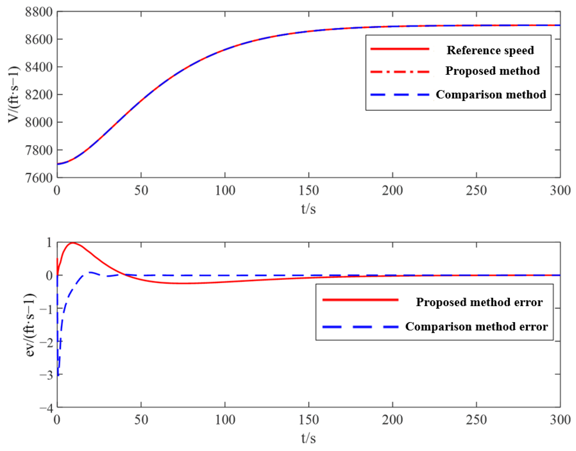
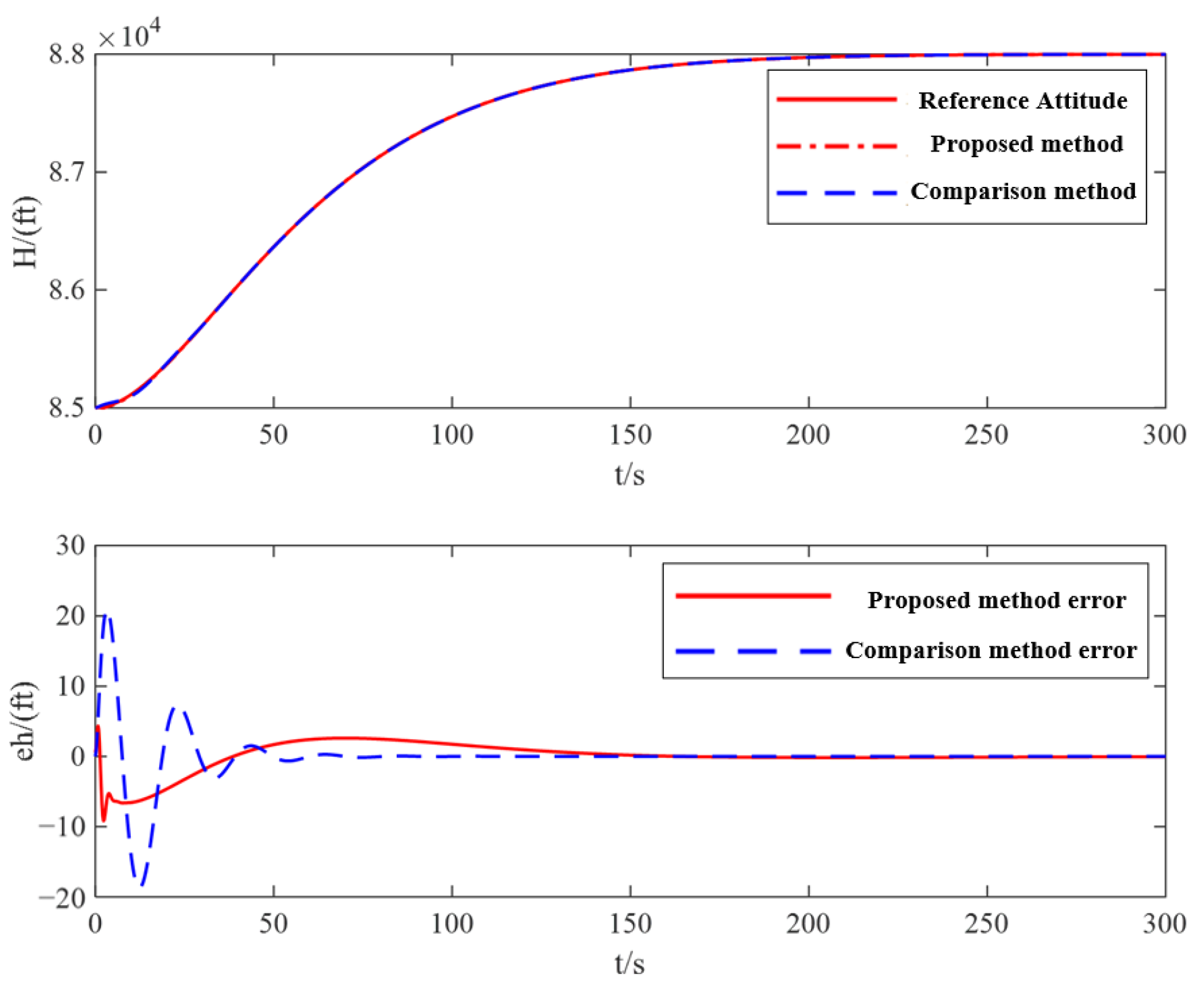
Scenario 1: due to systematic and random errors in speed sensors and height sensors, the initial error $e_V=0.5 \mathrm{ft}/\mathrm{s}$, $e_h=20 \mathrm{f}\mathrm{t}$ is considered, and 20% aerodynamic parameter perturbation and unknown external disturbances are added on this basis, i.e., $C=C_0\left(1+0.2\sin \left(0.1\pi t\right)\right)$, $C_0$ is the nominal aerodynamic parameter.

The simulation results of Scenario 1 are visually depicted in Figure 8, Figure 9, Figure 10 and Figure 11. These figures comprehensively compare the methodology proposed in this paper and the method employed for comparison. Both approaches demonstrate the ability to achieve stable instructions tracking, ensuring that the desired trajectories are followed. However, upon closer examination of Figure 8 and Figure 9, it becomes evident that the technique introduced in this article excels in tracking performance, particularly concerning height and speed. The tracking error and error fluctuation are notably within a smaller range when employing the method outlined in this research. The maximum error fluctuation for both speed and height is substantially reduced by more than 50%, signifying a considerable improvement in precision and consistency. Figure 10 and Figure 11 reveal that the absolute value of state quantities, denoted as $\gamma , \alpha , Q$, closely aligns with the comparison method, but the rate of convergence is significantly accelerated when utilizing the approach proposed in this paper. This acceleration signifies a more rapid adjustment and adaptation of the system to changing conditions, ultimately contributing to enhanced tracking and control. Furthermore, the system input operates within the linear region of the actuator, ensuring its high feasibility and practicality in real-world applications. These simulation results underscore the superiority of the proposed methodology in achieving more precise and reliable control in the context of hypersonic aircraft.

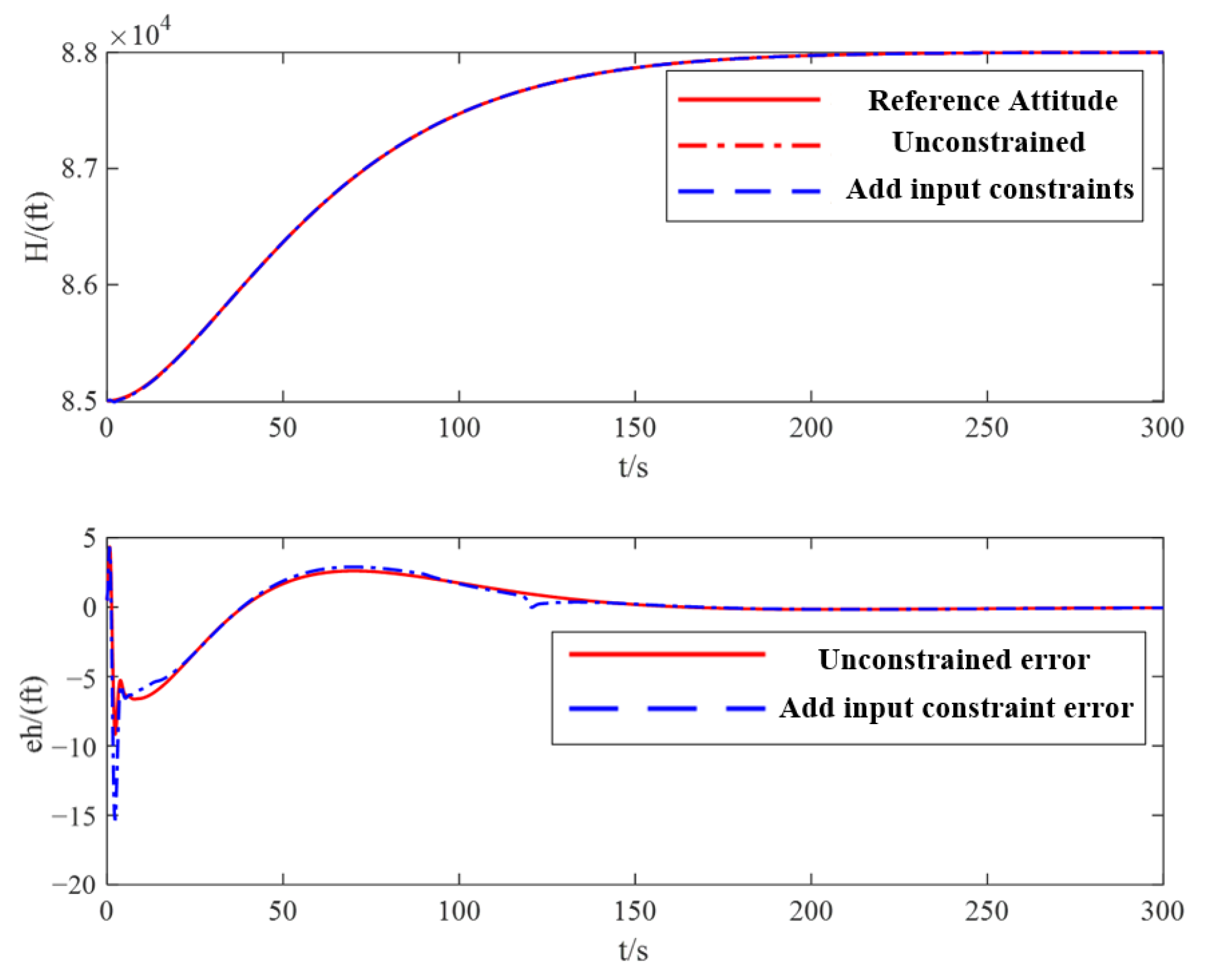
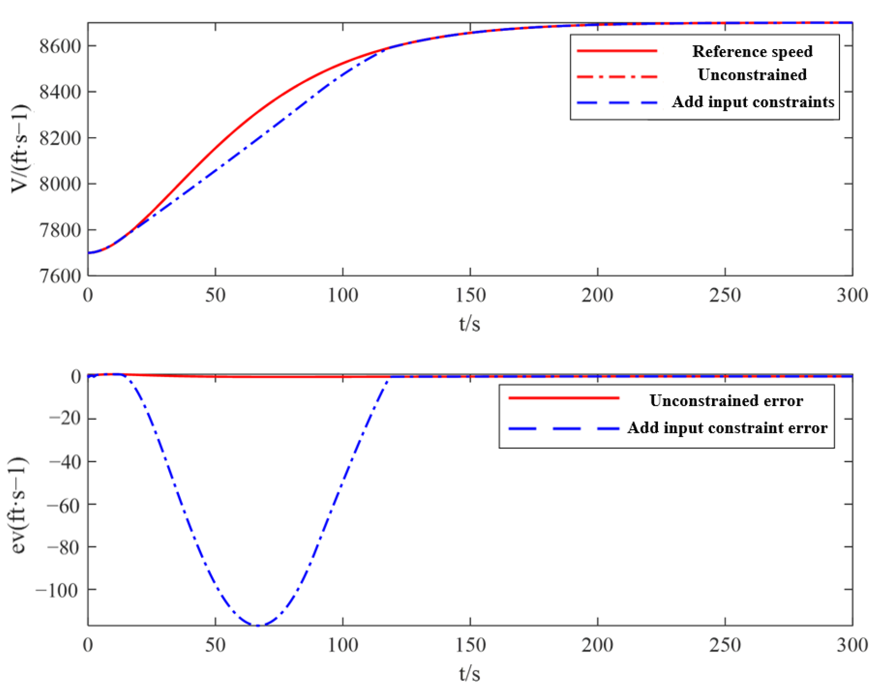
Scenario 2: considering the same initial error in Scenario 1, consider the more severe input saturation constraint of the actuator, $\mathrm{\Phi }\in [0.05,0.5]$, ${\delta }_e\in [-{15}^{\circ },{15}^{\circ }]$.

The simulation results for Scenario 2 are visually presented in Figure 12, Figure 13, Figure 14, Figure 15 and Figure 16, offering a comprehensive analysis of the performance under specific conditions. Figure 12 and Figure 13 shed light on the behavior in the presence of severe input saturation constraints. Despite the possibility of resulting in a speed error of 1.5%, it is noteworthy that the convergence speed exhibits a remarkable 20% improvement, indicating the ability of the proposed approach to adapt and adjust rapidly in the face of challenging conditions. Moreover, the error remains small for height, demonstrating the capability to achieve fast and stable tracking, even under such constraints. 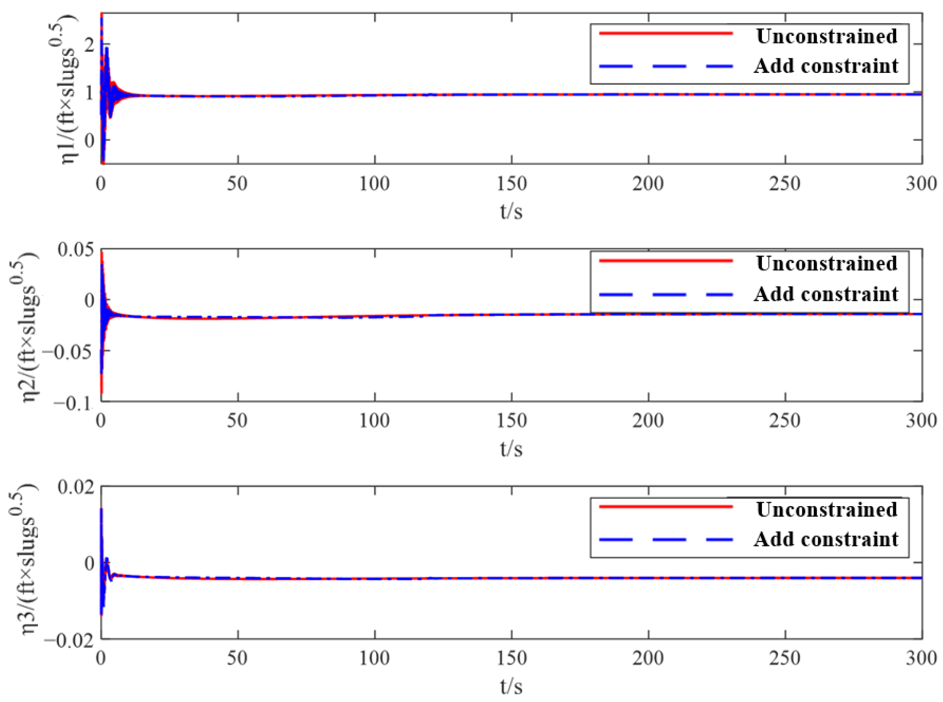Figure 14 and Figure 15 provide insights into the impact of severe saturation constraints on the system’s behavior and elastic states. Such constraints can induce inevitable fluctuations in both the system state quantity and the elastic state quantity. However, the compensation effect of the anti-saturation auxiliary system comes to the forefront, ensuring that these fluctuations do not exceed 15%. This places them well within an acceptable range, signifying the effectiveness of the anti-saturation auxiliary system in stabilizing the system and maintaining control over potentially erratic behaviors.

Furthermore, the effectiveness of the anti-saturation auxiliary system is further underscored by the input curve of the control system, as depicted in Figure 16. This figure illustrates how the system input operates in response to the challenging conditions posed by severe saturation constraints. The system effectively compensates for these constraints, maintaining control and stability, thus providing empirical evidence of the anti-saturation system’s effectiveness in overcoming limitations and maintaining reliable control.

4. Conclusions

In this study, the integration of RBFNN theory and adaptive control theory, specifically within input saturation constraints, has led to the development of an RBFNN adaptive controller and an anti-saturation auxiliary system for hypersonic vehicle control, ultimately unveiling a groundbreaking approach to hypersonic vehicle control. The simulation results we have obtained indicate the remarkable efficacy of this novel scheme, elevating the significance and potential applications of this research. Key conclusions drawn from this study are as follows:

(1)

Implementing the RBFNN adaptive controller has yielded significant quantifiable results. Notably, it has led to a remarkable reduction in the maximum error fluctuation of speed and height, with a decrease of over 50%. This outcome underscores the controller’s effectiveness in improving tracking accuracy and stability within the control system, contributing to its robustness in dealing with parameter uncertainties and disturbances.

(2)

The anti-saturation auxiliary system has shown noteworthy quantitative results when operating under severe input saturation constraints. Although such limitations may lead to a speed error of 1.5%, this auxiliary system has demonstrated an impressive 20% improvement in convergence speed. These results indicate the system’s resilience in ensuring precise tracking, even in scenarios characterized by severe input saturation, highlighting its potential to mitigate the effects of saturation constraints and enhance control system performance.

The achievements of this research not only advance the field of hypersonic vehicle control but also hold the potential to foster practical applications. By reducing error fluctuations and enhancing convergence speed, this work significantly improves the adaptability and robustness of control systems in hypersonic vehicles, ultimately enhancing their real-world performance. However, due to the significant cost and safety constraints associated with conducting experiments on actual hypersonic vehicles, we plan to employ a semi-physical simulation approach to validate our results in future research endeavors. The controlled environment facilitates a systematic exploration of performance under various conditions, contributing to a comprehensive understanding. Additionally, semi-physical simulations allow tailored and realistic validation for hypersonic flight challenges. In conclusion, future semi-physical simulations are essential for a robust assessment of the proposed controller, aligning with the unique challenges of hypersonic flight.

References

1. Bolender, M.A.; Doman, D.B. Nonlinear Longitudinal Dynamical Model of an Air-Breathing Hypersonic Vehicle. J. Spacecr. Rocket. 2007, 44, 374–387. [Google Scholar] [CrossRef]
2. Zhang, Y.; Huang, X.; Lu, K.; Bai, W.; Huang, W. Research Progress and Prospect of the Hypersonic Flight Vehicle Control Technology. J. Astronaut. 2022, 43, 866–879. [Google Scholar]
3. Sun, C. Development status, challenges and trends of strength technology for hypersonic vehicles. Acta Aeronaut. Astronaut. Sin. 2022, 43, 527590. [Google Scholar]
4. Zinnecker, A.; Serrani, A.; Bolender, M.; Doman, D. Combined reference governor and anti-windup design for constrained hypersonic vehicles models. In Proceedings of the AIAA Guidance, Navigation, and Control Conference, Chicago, IL, USA, 10–13 August 2009; p. 6283. [Google Scholar]
5. Li, X.; Li, G.; Zhao, Y.; Kang, X. Fuzzy-Approximation-Based Prescribed Performance Control of Air-Breathing Hypersonic Vehicles with Input Constraints; SAGE Publications: London, UK, 2020. [Google Scholar]
6. Zhu, J.; Chen, W.; Ma, H.; Yang, Z. Adaptive backstepping control of a flexible hypersonic vehicle with input saturations. J. Harbin Inst. Technol. 2018, 50, 102. [Google Scholar]
7. Si-Yuan, Z.; Xiao-Bing, L.I.; Yang-Guang, H.E.; Xing-Ge, L.I. Design of Adaptive Inversion Control for a Hypersonic Vehicle. In Proceedings of the 2018 IEEE 3rd Advanced Information Technology, Electronic and Automation Control Conference (IAEAC), Chongqing, China, 12–14 October 2018; pp. 1829–1834. [Google Scholar]
8. An, H.; Guo, Z.; Wang, G.; Wang, C. Neural adaptive control of air-breathing hypersonic vehicles robust to actuator dynamics. ISA Trans. 2021, 116, 17–29. [Google Scholar] [CrossRef]
9. Hu, Q.; Meng, Y. Adaptive backstepping control for air-breathing hypersonic vehicle with actuator dynamics. Aerosp. Ence Technol. 2017, 67, 412–421. [Google Scholar] [CrossRef]
10. Ding, Y.; Wang, X.; Bai, Y.; Cui, N. Novel anti-saturation robust controller for flexible air-breathing hypersonic vehicle with actuator constraints. ISA Trans. 2020, 99, 95–109. [Google Scholar] [CrossRef]
11. Ding, Y.; Yue, X.; Liu, C.; Dai, H.; Chen, G. Finite-time controller design with adaptive fixed-time anti-saturation compensator for hypersonic vehicle. ISA Trans. 2021, 122, 96–113. [Google Scholar] [CrossRef]
12. Chen, H.; Zhou, J.; Zhou, M.; Zhao, B. Nussbaum gain adaptive control scheme for moving mass reentry hypersonic vehicle with actuator saturation. Aerosp. Sci. Technol. 2019, 91, 357–371. [Google Scholar] [CrossRef]
13. Gao, S.; Ning, B.; Dong, H. Fuzzy dynamic surface control for uncertain nonlinear systems under input saturation via truncated adaptation approach. Fuzzy Sets Syst. 2016, 290, 100–117. [Google Scholar] [CrossRef]
14. Sun, J.G.; Li, C.M.; Guo, Y.; Wang, C.Q.; Peng, L. Adaptive fault tolerant control for hypersonic vehicle with input saturation and state constraints. Acta Astronaut. 2019, 167, 302–313. [Google Scholar] [CrossRef]
15. Bu, X.; Wu, X.; Ma, Z.; Zhang, R.; Huang, J. Novel auxiliary error compensation design for the adaptive neural control of a constrained flexible air-breathing hypersonic vehicle. Neurocomputing 2016, 171, 313–324. [Google Scholar] [CrossRef]
16. Hu, Q.; Meng, Y.; Wang, C.; Zhang, Y. Adaptive Backstepping Control for Air-Breathing Hypersonic Vehicles with Input Nonlinearities. Aerosp. Sci. Technol. 2017, 73, 289–299. [Google Scholar] [CrossRef]
17. Fiorentini, L.; Serrani, A.; Bolender, M.A.; Doman, D.B. Nonlinear Robust Adaptive Control of Flexible Air-Breathing Hypersonic Vehicles. J. Guid. Control Dyn. 2009, 32, 401. [Google Scholar] [CrossRef]
18. Sun, J.; Yi, J.; Pu, Z.; Liu, Z. Adaptive Fuzzy Nonsmooth Backstepping Output-Feedback Control for Hypersonic Vehicles With Finite-Time Convergence. IEEE Trans. Fuzzy Syst. 2019, 28, 2320–2334. [Google Scholar] [CrossRef]
19. Bu, X.; Wu, X.; Wei, D.; Huang, J. Neural-approximation-based robust adaptive control of flexible air-breathing hypersonic vehicles with parametric uncertainties and control input constraints. Inf. Sci. 2016, 346, 29–43. [Google Scholar] [CrossRef]
20. Parker, J.T.; Serrani, A.; Yurkovich, S.; Bolender, M.A.; Doman, D.B. Control-Oriented Modeling of an Air-Breathing Hypersonic Vehicle. J. Guid. Control Dyn. 2007, 30, 856–869. [Google Scholar] [CrossRef]
Figure 1. Longitudinal geometric configuration.
Aerospace 11 00108 g001
Figure 2. Schematic diagram of RBFNN structure.
Aerospace 11 00108 g002
Figure 3. RBFNN applied to the controller principle flowchart.
Aerospace 11 00108 g003
Figure 4. Overall control structure diagram.
Aerospace 11 00108 g004
Figure 5. Speed subsystem control structure diagram.
Aerospace 11 00108 g005
Figure 6. Height subsystem control structure diagram.
Aerospace 11 00108 g006
Figure 7. RBFNN control system.
Aerospace 11 00108 g007
Figure 8. Speed tracking (Scenario 1).
Aerospace 11 00108 g008
Figure 9. Height tracking (Scenario 1).
Aerospace 11 00108 g009
Figure 10. State variables (Scenario 1).
Aerospace 11 00108 g010
Figure 11. System input curve (Scenario 1).
Aerospace 11 00108 g011
Figure 12. Speed tracking (Scenario 2).
Aerospace 11 00108 g012
Figure 13. Height tracking (Scenario 2).
Aerospace 11 00108 g013
Figure 14. State variables (Scenario 2).
Aerospace 11 00108 g014
Figure 15. Elastic state (Scenario 2).
Aerospace 11 00108 g015
Figure 16. System input curve (Scenario 2).
Aerospace 11 00108 g016