Abstract
Urban air mobility is expected to play a role in improving transportation of people and goods in growing urban areas while contributing to sustainable urban growth and zero-emissions future aviation. The research presented herein computationally investigated the performance of control laws for a generic Urban Air Taxi (UAT) subjected to empirically-developed urban airflow disturbances. This involved developing a representative flight dynamics model of a UAT in steady level cruise flight with an inner-loop autopilot. Active Disturbance Rejection Control (ADRC) and Proportional-Integral-Derivative (PID) control laws were implemented to investigate the controlled and uncontrolled acceleration responses and compare them to the acceleration limits in ISO 2631. Using a linear flight dynamics model, ADRC demonstrated improved performance over PID control with equal initial tuning effort. PID was able to reduce passenger accelerations to unharmful, though still uncomfortable, levels while ADRC further reduced the lateral accelerations to comfortable levels.
1. Introduction
There is increased interest in aircraft operations in unserved and underserved local, regional, intraregional, and urban areas with the goal of improved and sustainable passenger and cargo transportation. This new area in aviation is being referred to as Advanced Air Mobility (AAM) and Urban Air Mobility (UAM) [1]. It is predicted that 60% of the world’s population will live in urban areas by 2030 [2]. This increase in urban population and access to new aerospace technology is contributing to increasing aircraft operations over and within cities. UAM operations have already been conducted, where in October 2021, a fully autonomous drone performed the first lung transport in a dense urban setting [3].
The challenges for UAM include, but are not limited to, GPS reception issues near buildings [4], cybersecurity risks with data transmission [5], developing new air-traffic control technologies [6,7], and noise and safety requirements [5]. One aspect of the urban environment that affects aircraft performance and safety are turbulent wind conditions [8,9,10]. These conditions occur in the urban environment and form due to the general wind interaction with the surface roughness of the surrounding area as well as the specific flow interaction with tall buildings. Turbulence can severely affect the flight performance of aircraft and will play a significant role in how aircraft operations are regulated and conducted in the urban environment.
The UAM ConOps [11] identifies that operators will need to understand the constraints the wind conditions have on UAM operations. This includes knowing what wind conditions will limit the ability of the aircraft to perform safe operations. The FAA’s Engineering Brief No. 105 for Vertiport Design describes how turbulence due to wind interacting with surrounding structures will need to be considered when designing Vertiports because of its effect on Vertical Take-Off and Landing (VTOL) operations [12]. The report identifies that if turbulence cannot be mitigated then operational constraints will be required. These reports have identified that understanding the effect of wind and turbulence on UAM aircraft performance is critical to safe operations. This leads to an open question about what wind and turbulence conditions, or levels, would limit UAM operations in certain areas.
It is expected that, in the long term, UAM vehicles will be either entirely autonomously controlled or be piloted by a human through a Stability Augmentation System (SAS) and, in the short term, Remotely Piloted Aircraft Systems (RPAS) will conduct beyond visual line of sight operations. Both will require robust control systems to ensure safe operations. To realize a successful, safe, and sustainable future with UAM, novel control concepts must be analysed under the conditions that correspond to those which UAM vehicles are expected to operate within.
Flight dynamics models are often required to develop suitable flight controllers for aircraft. This is certainly the case for the new generation of UAM aircraft. UAM aircraft concepts have been analysed with various configurations, such as lift + cruise or tilt-rotor, to identify the mission set they are suited to perform [13]. Multi-Disciplinary Design Optimization (MDO) methods to develop electric Vertical Take-off and Landing (eVTOL) aircraft designs have been proposed. An example of this is the Possibility-based Design Optimization (PBDO) method for MDO of an eVTOL tilt-wing aircraft [14]. Concept UAM aircraft designs, such as these, can be used to provide flight dynamics models for the initial design of flight control systems.
Previous investigations have implemented methods to design Proportional-Integral-Derivative (PID) control flight controllers. The Army Research Lab (ARL) has presented a simulation environment that can be used to implement and evaluate PID controllers for micro air vehicles [15]. Rostami et al. [16] have presented a multi-objective PID optimization method using a Genetic Algorithm for the lateral control of a twin-engine aircraft. Simulation frameworks and optimization methodologies such as these provide methods that could be applied to control system design for UAM operations.
In this paper, the development of a generic Urban Air Taxi (UAT) flight dynamics model in the steady-level cruise phase of operation for the purpose of evaluating the performance of different inner-loop controllers for UAM applications is described. Two inner-loop flight controllers were designed. The first controller utilizes classical Proportional-Integral-Derivative (PID) control, while the second controller uses the concepts of Active Disturbance Rejection Control (ADRC). The controllers were tuned through input step perturbations of the flight dynamics model from its steady-level cruise condition. Utilizing an empirically-developed urban airflow model [10], the turbulent airflow conditions corresponding to a dense urban centre were created. The flight dynamics model and its inner-loop controllers are then immersed in the synthesized turbulent urban airflow conditions to assess the performance of the UAT with and without control in the urban setting. Conclusions and future research recommendations are then drawn based on the comparison of the acceleration limits in ISO 2631 and the frequency-weighted Root Mean Square (RMS) accelerations the UAT experiences while subjected to the urban airflow disturbances.
2. Background
Turbulent wind conditions in urban areas that could affect the flight performance of UAT have been discussed in References [8,9,10]. Urban infrastructure can have a major impact on the flow in cities; for example disturbed flow can exist at a distance from a building up to three times the height of that building [8]. Scientists from NASA Ames took wind measurements at certain points in downtown San Francisco and used these data to model the wind and roughly represent the variable wind and turbulent conditions [9]. They found that it could be difficult and dangerous to operate UAM type vehicles manually at certain locations in the city. It may be possible for significant turbulence to affect a UAM vehicle approaching a city from the downwind direction or travelling over a city at lower altitude. Realistic flow field models need to be generated and applied to UAM flight models and the vehicle performance analysed with and without automatic controllers. Variable winds and turbulence have been used in flight dynamics models that generally use Power-Spectral-Density (PSD) plots based on the Dryden or Von-Karman turbulence models [17,18,19]. In this work, PSD plots developed using empirical measurements in a wind tunnel [10] were used to synthesize the disturbance input for the UAM flight dynamics model.
Improving passenger comfort and reducing aircraft structural loads can be accomplished through gust load alleviation techniques. These techniques use sensed information about a wind gust to adjust actuators to reduce the loads experienced by the aircraft. The oncoming gust can be sensed using, Doppler LIDAR [20,21], angle of attack sensors [22], or aircraft mounted accelerometers [23]. The gust information gathered by these sensor systems can be used with active control techniques to actuate lifting surfaces [20,24] or flow control devices [23,25] which reduce the change in aircraft lift coefficient and wing bending moments. Passive control techniques have also been demonstrated, which accomplish the same goal of alleviating gust loading to the aircraft [26]. These techniques play a crucial role in improving aircraft performance by reducing unwanted aircraft motion that can effect passenger comfort or safety and limiting structural loading which allows for the reduction of aircraft weight by reducing structural requirements [22,23]. UAM aircraft will likely encounter turbulent wind conditions that will affect aircraft performance. Gust alleviation techniques will improve the safety, comfort, and efficiency of these aircraft.
It is expected that a UAM aircraft will use a SAS to augment the pilot command and maintain control of the aircraft. Robust controller designs suitable for aerospace applications have been investigated and applied to various types of UAM vehicles ranging in size from small unmanned drones to large passenger carrying UAT [18,27,28,29,30] and often make use of a system specific model. ADRC was chosen as the novel controller to investigate because it shows positive results in robust control of non-linear systems [31]. Furthermore, ADRC is not a model based controller and does not require a highly accurate system model to ensure good controller performance [31]. These qualities are a benefit in the aerospace industry where systems can be highly non-linear and developing highly accurate models is time consuming and expensive. ADRC may allow for faster development of robust controllers that meet the precise requirements of the aerospace industry. The performance of the UAT with and without control is compared to the health and comfort acceleration limits laid out in ISO 2631 [32].
The ISO 2631 standard was chosen because it provides both quantitative values for acceleration for various discomfort levels and provides accelerations that are potentially hazardous to ones health. This standard has also been used to asses passenger comfort in large passenger aircraft [33,34,35]. Figure 1 shows the health guidance caution zones in weighted acceleration. The area between each set of dotted lines describes the health guidance caution zone, where each set of dotted lines corresponds to alternative equations relating time dependence of acceleration exposure [32]. The comfort acceleration limits [32] are as follows:
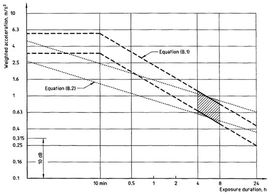
Figure 1.
Health guidance caution zones from ISO 2631-1. Reproduced from [36].
- Less than 0.315 , not uncomfortable;
- 0.315 to 0.63 , a little uncomfortable;
- 0.5 to 1 , fairly uncomfortable;
- 0.8 to 1.6 , uncomfortable;
- 1.25 to 2.5 , very uncomfortable;
- Greater than 2.5 , extremely uncomfortable.
3. Model, Disturbance, and Controller Development
To investigate the accelerations experienced by the UAT being subjected to urban airflow conditions, a flight dynamics model of a prototype UAT is developed. The urban airflow disturbance is applied as an input to the model and the response simulated using Simulink. PID control and ADRC laws are implemented as inner-loop controllers to investigate the controlled as well as the uncontrolled responses.
For the development of a generic UAT flight dynamics model linear aerodynamics are considered, which are applied through potential flow and thin airfoil theories. Linear aerodynamic modelling methods are used because they provide a straightforward method for initial model development and will provide aircraft dynamics that are representative of level cruise flight. These methods lead to model development with simple approximations that yield an adequate representation of the flight dynamics [37]. This provides adequate system dynamics for the comparison of the performance provided by the two different flight controllers. In the development of the model, unsteady aerodynamics are neglected to simplify aerodynamic modelling, while simple methods are used for the inertia estimation as specific mass distribution information is unavailable. These modelling methods and assumptions lead to a flight dynamics model that is representative of a generic UAT, which is based on the Bell Nexus 4EX aircraft. Although the flight dynamics model may not necessarily be an exact representation of the actual Nexus’ flight dynamics, the model does provide system dynamics that are appropriate to compare the performance of the two controllers against each other.
3.1. Selection of the UAT Platform for Generic UAT Flight Dynamics Model
Several urban air taxi prototypes were considered including the vehicles in development by Joby Aviation [38], Lilium [39], Airbus [40], Volocopter [41], and Bell Textron [42]. Bell has proven experience with VTOL and Short Take-Off and Landing (STOL) type aircraft in both development and product deployment. The V-22 Osprey is a VTOL/STOL capable aircraft operated by the United States military used for special operations, air assault, and transportation of passengers and cargo [43]. Bell also developed the X-22 for the Unites States Navy which started development in the 1960’s [44]. This aircraft used four articulating ducted fans to produce lift or thrust, and had fixed lifting surfaces for horizontal flight, which is similar in design to the proposed UAT concept the Nexus 4EX shown in Figure 2. The relatively simple geometry of the Bell Nexus and availability of close up images aids in the estimation of geometric parameters. For these reasons, the Bell Nexus 4EX was chosen as the basis to estimate the model parameters for the generic UAT layout. This generic UAT was used to generate a representative flight dynamics model for the purposes of evaluating the flight controllers.
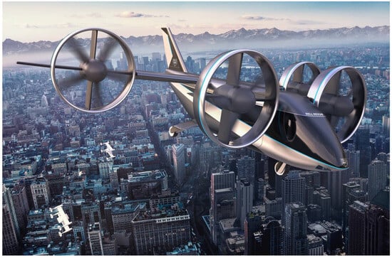
Figure 2.
Bell Nexus 4EX [42].
3.2. Geometric and Inertial Parameter Estimation
Obtaining the geometric and the inertial parameters is a prerequisite to estimating the aerodynamic derivatives and parameters. Figure 3 shows the generic UAT layout that was created to identify the geometric parameters. The parameters were estimated using available images of the Bell Nexus 4EX that were then scaled using a reported duct diameter of eight feet [45]. The estimated wing and canard geometric parameters are shown in Table 1.
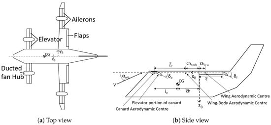
Figure 3.
Generic UAT layout, where , , and are the body frame x, y, and z directions, is the wing-body angle of attack, is the mean aerodynamic chord, h is the percent location of the centre of gravity, is the percent location of the main wing neutral point, is the percent location of the wing-body neutral point, is the distance between the main wing and canard aerodynamic centres, is the distance between centre of gravity and canard aerodynamic centre, is the elevator deflection angle, and is the flap deflection angle.

Table 1.
Geometric parameters for main wing and canard, where b is the span and S is the planform area.
The inertial parameters were estimated using a simple uniform density rectangular prism with similar dimensions to the body of the Bell Nexus 4EX. The inertia estimates were improved by using available aircraft component weight group mass fractions for a similar aircraft, the Bell X-22a, taken from [46]. The body dimensions of the generic UAT were estimated as 1.868 m, 1.564 m, and 8.431 m for the height (H), width (W), and length (L) respectively. The mass fractions for the power plant group and wing group were taken from [46] and used to calculate a mass to lump at each duct motor location, those values are 0.35 and 0.054 respectively.
The mass moment of inertia, I, about each of the rectangular prism principal axes, , , and respectively, were calculated using [47],
where m is the mass which was taken as 3175 kg [45]. The mass associated with the power plant group and wing group was divided between the four ducted fans and lumped at the point locations of the center of each hub. The remaining mass was treated as the mass of the fuselage. The mass moment of inertia about each axis due to the point masses was added to the principal axes mass moment of inertia for the fuselage. The estimated overall principal moments of inertia are listed in Table 2.
Table 2.
Mass moments of inertia about the principal axes.
3.3. Aerodynamic Parameter Estimation
The aerodynamic parameters and derivatives were obtained using the estimated geometric parameters along with analytic and empirically-developed equations taken from [48].
3.3.1. Lift-Curve Slope Coefficient Estimation
The lift-curve slope coefficients for the aircraft lifting surfaces were estimated based on the two-dimensional lift-curve slope, , obtained using potential flow and thin-airfoil aerodynamic theorems. These are are normally used in preliminary aircraft sizing and conceptual design as reported in [37] and found using,
where is the wing thickness ratio and is the sweepback angle of the leading edge. The two-dimensional lift-curve slope was used to estimate the three-dimensional lift-curve slope, a, using [37],
where is the aspect ratio. The lift-curve slope coefficients for the wing-body, canard, and vertical stabilizer are estimated using the geometric parameters for each surface with Equations (4) and (5). Their values are presented in Table 3 where the subscripts , c, and F refer to the wing-body, canard, and vertical tail surfaces respectively.
Table 3.
Lift-curve slope coefficients.
3.3.2. Longitudinal Static Analysis
A longitudinal static analysis was conducted to determine the static longitudinal stability derivatives and UAT reference condition during steady level flight. In the reference flight condition, the UAT is said to be trimmed with the overall lift coefficient being given by [48],
where W is the aircraft weight force, is the air density, V is the UAT airspeed, and S is the main wing planform area. The trimmed lift coefficient is then employed in Equation (7) along with the overall aerodynamic moment coefficient of the aircraft at zero lift, , in steady level-flight to obtain the trimmed aircraft angle of attack and elevator deflection such as [48],
The lift and moment with respect to angle of attack coefficients were estimated using Equations (8) and (9) where propulsive effects and downwash effects from the forward ducts and canard were neglected for simplicity.
In Equation (8), is the planform area of the canard and in Equation (9), h is the location of the centre of gravity and is the location of the overall UAT neutral point both as a percentage of the mean aerodynamic chord of the wing. The change in the lift and the moment coefficients due to elevator deflection, and , are estimated using
where is the elevator effectiveness coefficient and is the horizontal tail (canard) volume ratio relative to the aerodynamic centres of the canard and wing-body, which are estimated using the methods in [48]. The reference conditions are shown in Table 4.
Table 4.
Steady level-flight trim conditions.
Where is the elevator deflection angle, is the flap deflection angle, is the angle of attack relative to the zero-lift line, is the angle of attack relative to the body x-axis, and is the longitudinal static margin. The cruise velocity, V, for the UAT is taken as 150 mph [45], and the air density, , is taken as 1.19 .
3.3.3. Estimation of Stability Derivatives
The estimation of the stability, or aerodynamic, derivatives is accomplished using analytical, semi-empirical and empirical methods obtained from the USAF Datcom database and the British Aeronautical Society [48]. The stability derivatives are estimated as non-dimensional values which are dimensionalised based on the UAT geometries and steady-flight reference conditions using dimensionalization equations from [48]. The estimated non-dimensional stability derivatives are given in Table A1 and Table A2. The longitudinal and the lateral dynamics can be treated separately due to the symmetry of the aircraft about the aircraft body x–z plane. Table 5, Table 6, Table 7 and Table 8 give the entries for the longitudinal and lateral state and control matrices which contain the dimensional stability derivatives. The non-dimensional control derivatives are estimated using the methods provided in [48] and are listed in Table A3. The upper-case letters X, Z, and Y refer to the forward, vertical, and lateral force components while M, N, and L represents the pitching, the yawing, and the rolling moments. The lower-case subscripts give the variable to which the force or moment is affected by. In the longitudinal direction those values are the forward airspeed u, the vertical speed w, the pitch rate q, and the rate of change of the vertical airspeed . Unsteady effects, captured in , were neglected in this study due to the high speed of the aircraft compared to the wind speed disturbance fluctuations. In the control matrix, the subscript c represents the control variable. In the lateral direction, the subscript values are the lateral airspeed v, the roll rate p, and the yaw rate r. In Table 7 and Table 8, , , and are the moments and product of inertia about the UAT stability axes which were calculated from the principal axis moment of inertia given in Table 2.
Table 5.
Longitudinal state (A) matrix entries.
Table 6.
Longitudinal control (B) matrix entries.
Table 7.
Lateral state (A) matrix entries.
Table 8.
Lateral control (B) matrix entries.
3.4. State-Space Model
The model for the generic urban air taxi is created using the linearized, small disturbance state-space model derived in [48], which follows the form
where x is the state variable vector, is the control input, and is the rate of change of the state variables. The wind disturbance due to the urban airflow impacts the state of the UAT since it changes the relative airspeed in Equation (12) and as pictorially depicted in Figure 4, which shows the system representation of the flight dynamics model in a block diagram format.
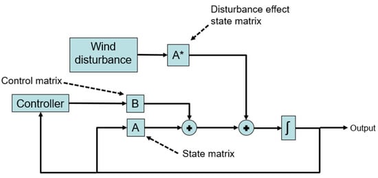
Figure 4.
Block diagram showing arrangement of state-space matrices, controller, and wind disturbance for simulation development.
Stability Analysis
A stability analysis was conducted based on the longitudinal and the lateral state matrices to determine the control fixed dynamic stability characteristics of the generic UAT. The stability was assessed using the eigenvalues obtained from the characteristic polynomial for the system formed using
where is variable used to represent the roots of the polynomial and I is the identity matrix, which is used to introduce into the matrix form.
The longitudinal dynamics were determined to have stable long and short period modes. The lateral dynamics were determined to have stable rolling convergence and Dutch roll modes while the spiral mode was found to be unstable. For this investigation, the instabilities were stabilized by conducting a sensitivity analysis on the stability derivatives which led to altering the rolling moments with respect to yaw rate and lateral velocity, and respectively, as well as altering the lateral force with respect to lateral velocity, . The , , and stability derivatives were scaled to 5%, 120%, and 210% of their original values respectively. Modifying these parameters allowed for effects such as the dihedral effect due to a high wing location to be included even though it was not included in the original estimation of the parameters. The stability of each mode was assessed considering the stability requirements in the Transport Canada airworthiness manual Chapter 523 [49]. Equivalent regulations can be found in the FAA part 23 and EASA CS-23 documents. The eigenvalues and characteristic times for each mode are shown in Table 9.
Table 9.
Longitudinal and lateral eigenvalues, periods, and damping times.
The damping ratios for longitudinal and lateral modes are shown in Table 10. The damping ratios and natural frequencies are compared to the category B flight phase to determine handling quality level, which are identified in MIL-F-8785-C [50]. It should be noted that the spiral mode is excluded from Table 10 because it has been stabilized and hence does not have a time to double amplitude. All modes achieve a handling quality level of 1 apart from the Dutch Roll mode, which is at level 2. The results of the tuned controllers will demonstrate the this can be improved to a level 1 through the use of the automatic flight controllers.
Table 10.
Handling quality levels of uncontrolled longitudinal and lateral modes.
3.5. Urban Airflow Disturbance
The urban airflow disturbance is created using experimental data taken from the experiment described by Al Labbad et al. [10] which focused on a section of the Toronto city downtown area. The experimental model was centred on the Hockey Hall of Fame and covered a circular area with a full scale radius of 242 m with a maximum full scale building height of 248 m. A CAD model of this area is shown in Figure 5. The green buildings in Figure 5 represent the site of future construction. These buildings were included in the south wind direction data but not in the west-south-west wind direction data.
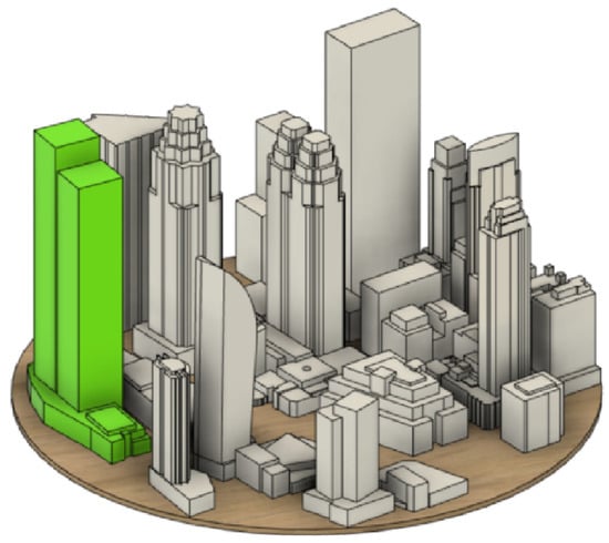
Figure 5.
Final sub-scale CAD model for city model. Reproduced from [51].
Eight different data points corresponding to different locations in the urban airspace are used to create the urban airflow disturbances where four points correspond to a south wind direction and the remaining four points correspond to a west-south-west wind direction. The south wind direction data points were measured at a full scale height of 105 m while the west-south-west wind direction data points were measured at a full scale height of 57 m. Although these heights are lower than that of the UAT cruise altitude, these data are used to provide worst case scenario disturbances to evaluate the flight controllers. These points, with the wind direction and turbulence intensity values in each coordinate direction, are shown in Figure 6 and Figure 7 respectively. The numbered points identify the data used to create the disturbances. These points were chosen because they show turbulence in each direction and have reasonable turbulence intensity in at least one direction. The RMS of the velocity signal in the u, v, and w directions for each point are shown in Table 11 to show the severity of the wind speed fluctuations.
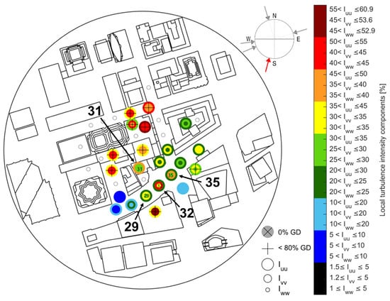
Figure 6.
South wind direction data points. Measurements taken at 105 m full scale above the ground. Reproduced with modifications from [51].
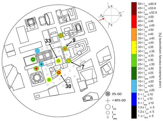
Figure 7.
West-south-west wind direction data points. Measurements taken at 57 m full scale above the ground. Reproduced with modifications from [51].
Table 11.
RMS of the velocity signal in the u, v, and w directions for each point.
The data corresponding to the change in the wind speed from its average value in each coordinate direction was presented as a Power-Spectral-Density (PSD) plot which was used to extract modal information to construct several harmonic signals using a Fourier series. A PSD plot for the variation in the lateral, v-direction, wind speed is shown in Figure 8. The PSD plots show the wind variation decreasing by approximately 2 orders of magnitude at 1 Hz; therefore the data are sectioned into three windows of equal width using 1 Hz as the maximum frequency. Three windows are selected to provide an initial disturbance case to demonstrate the potential of the ADRC flight controller, however this small number of windows only provides a simplified wind disturbance representation. The amplitude in the time domain is calculated using [52],

Figure 8.
PSD plot of lateral, v-direction, wind speed variation using data from Reference [51] for point 32.
Which was combined with [52],
to create the lateral velocity component as an example. In Equation (14), is the amplitude from the PSD plot and is the window width in terms of frequency. In Equation (15) the frequency for each mode, , was taken from the midpoint of each window and random values were used for the phase angles, . N is a variable representing the maximum number of modes, j is an index value, and t is the time variable. The modal information and windows are labelled on the plot in Figure 8. Figure 9 shows the results of applying Equation (15) to each wind direction and combining the modal information as a Fourier series to produce the time-series disturbance.
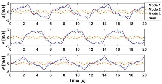
Figure 9.
Urban airflow disturbance for stream wise, u-direction, lateral, v-direction, and vertical, w-direction for point 32.
The wind disturbance is applied to the model by using equivalent longitudinal and lateral state matrices where the wind disturbance velocity, in the u, v, and w directions, are applied to the corresponding u, v, and w airspeed inputs of the matrices in the aircraft stability axis frame. The calculated response from these matrices is then added to the system response to determine the total system response.
3.6. Inner-Loop Controllers
ADRC and PID controller designs are used to create an autopilot with inner-loop control. The PID controller uses the following control law [53],
where e is the error, is the proportional gain, is the integral gain, is the derivative gain, t is time, is an integration parameter, and u is the calculated control input to the plant. Using simulations, different PID combinations were tested and it was chosen to use PID control for the elevator channel to control the pitch angle, proportional only (P) control for the rudder channel to control the yaw rate, and PID control for the aileron channel to control the bank angle. The rudder channel controller uses the yaw rate as the feedback signal and acts as a yaw damper. The PID gain values were iteratively adjusted individually while monitoring and minimizing the rise time, overshoot, and settling time in the responses. The PID controller gains for the control channels are shown in Table 12.
Table 12.
Controller parameter values.
ADRC consists of the transient profile generator, the non-linear weighted sum, and the Extended State Observer (ESO) which are combined through the control law represented by the system architecture in Figure 10 [53]. The transient profile generator takes a non-smooth changing set-point signal and provides smooth set-point and set-point derivative signals for error computation. The smooth signal is also meant to provide a smooth input signal to the plant which is easier to follow [53].
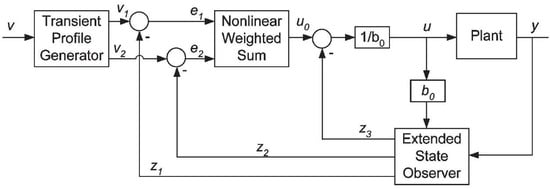
Figure 10.
ADRC system architecture. Reproduced from [53].
The transient profile generator is not included in this investigation as the set-point remains constant. The non-linear weighted sum is an alternative control law to the linear PID combination which was developed through simulation [53]. The ESO is a state observer which uses an additional state to capture the effects of unknown internal system dynamics and external system disturbances [53]. The non-linear weighted sum and the ESO use the continuous forms that are laid out in [53] and each control channel uses the same control design. The value for each of the ADRC parameters are shown in Table 12. The controller gains were tuned to minimize the rise time, overshoot, and settling time of the pitch angle, yaw rate, and bank angle when the system was subjected to a step input disturbance to the vertical and lateral wind speeds.
The mathematical implementation for ADRC flight controller that was used in the simulation is as follows. The ideal control signal is calculated with [53]
where and are controller parameters, and are the feedback error and error derivative signals, and is [53]
where the parameters in Equation (18) are calculated using the following list of equations from Reference [53]:
The ESO set-up is constructed following the one presented in Reference [53] and are:
where , , and are the state estimates; e is the error determined by the difference between the estimated state and the measured output y; , , and are the observer gains; and is a non-linear function taken from Reference [53] and described by:
where and are function tuning parameters. The final control signal is calculated using [53]
where is an estimate of the plant b coefficient [53]. For the ADRC autopilot, the ESO gains were set according to [53]
where in this controller implementation, h is set equal to . The controller parameters are then tuned following the order , , , and while aiming to minimise the rise time, overshoot, and settling time of the controlled system responses. The response of the controlled system parameters and control deflection angles to a unit step disturbance in the vertical airspeed, w, and lateral airspeed, v, are shown in Figure 11, Figure 12 and Figure 13. The responses show the ADRC flight controller performing better that the PID flight controller. All the control surface deflections are reasonably small such that linear aerodynamics assumption is still applicable to determine the induced aerodynamic forces. Figure 12 and Figure 13 demonstrate that the damping has been increased to move the Dutch Roll mode handling quality to level 1.
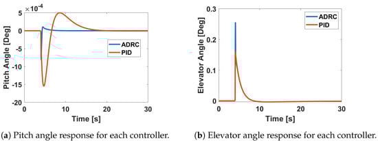
Figure 11.
Pitch and elevator angle response of UAT to step disturbance in vertical airspeed, w.
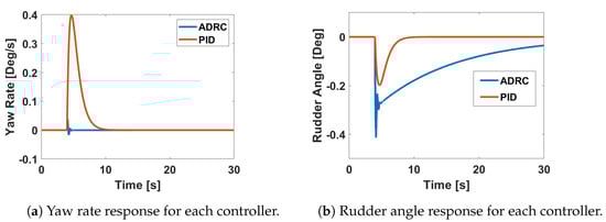
Figure 12.
Yaw rate and rudder angle response of UAT to step disturbance in lateral airspeed, v.
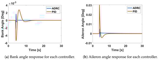
Figure 13.
Bank and aileron angle response of UAT to step disturbance in lateral airspeed, v.
4. Results
The UAT response to several urban airflow disturbances under PID and ADRC control, and in the uncontrolled mode, are presented here. As an example, the wind speed disturbance associated with data point 32 is shown in Figure 14. The pitch and elevator angles; yaw rates and rudder angles; and bank and aileron angles are shown in Figure 15, Figure 16 and Figure 17 respectively using the urban airflow data from point 32 identified in Figure 6.
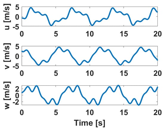
Figure 14.
Urban airflow wind disturbance for point 32.
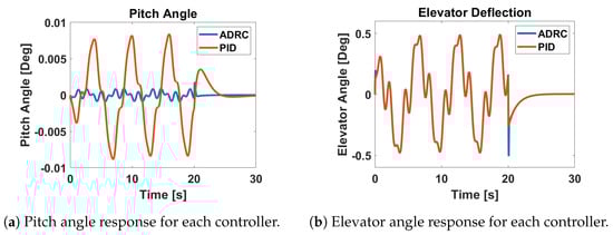
Figure 15.
Pitch and elevator angle response of the UAT to an urban airflow disturbance generated from point 32.
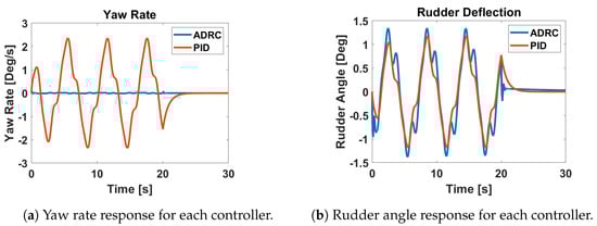
Figure 16.
Yaw rate and rudder angle response of the UAT to to an urban airflow disturbance generated from point 32.
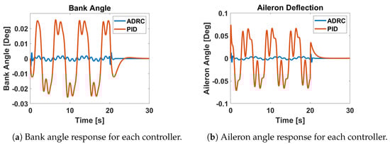
Figure 17.
Bank and aileron angle response of the UAT to to an urban airflow disturbance generated from point 32.
The results shown in Figure 15, Figure 16 and Figure 17 demonstrate the ability of the ADRC flight controller to outperform a PID controller when subjected to an urban airflow disturbance. This can be seen by the reduced magnitude of the pitch angle, yaw rate, and bank angle responses when using ADRC as compared to PID control. Both controllers produce control surface deflection magnitudes that are not excessive. It should be noted that Figure 15 and Figure 16 show the difference in the pitch angle and yaw rate to be large between the two controllers while the difference in the actuator deflections are not significant. For the pitch angle responses, the overall magnitude is quite small and the slight difference between the ADRC and PID elevator deflections would result in the difference observed in the pitch angle. The same is true in the yaw rate responses where the small difference in the rudder deflection produced by each controller would result in the difference observed in Figure 16.
To further assess the ability of the ADRC flight controller, the frequency weighted accelerations are computed for all eight urban airflow points both in the vertical and lateral directions according to the ISO 2631 standard. These results are shown for the south wind direction in Figure 18 and for the west-south-west wind direction in Figure 19.
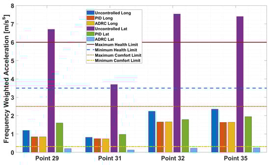
Figure 18.
Frequency-weighted accelerations for the uncontrolled, PID- and ADRC-controlled UAT operating under south wind direction.
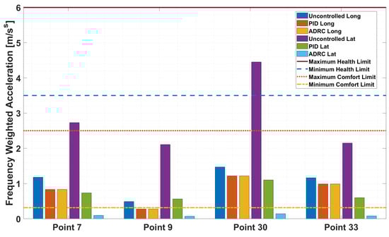
Figure 19.
Frequency-weighted accelerations for the uncontrolled, PID- and ADRC-controlled UAT operating under west-south-west wind direction.
Figure 18 and Figure 19 demonstrate that the wind direction can have a significant effect on the accelerations experienced by the UAT in the urban environment. This is shown by the overall higher accelerations when uncontrolled in the south wind direction results as compared to the west-south-west wind direction results. Both figures also demonstrate that the ADRC flight controller is able to significantly reduce the accelerations experienced in the lateral direction for both wind directions as compared to the PID flight controller. The lateral ADRC results are all below the minimum comfort acceleration levels while all the PID lateral acceleration results are well within the discomfort acceleration range. The longitudinal acceleration results for the ADRC and PID flight controllers are essentially equal, which is due to single channel pitch angle control for both controllers.
To asses the ability of the ADRC flight controller in a different flight condition, the longitudinal and lateral state matrices were recalculated for a reduced cruise speed of 120 mph as compared to the stated cruise speed of 150 mph and the flap angle was increased to 10 degrees. The same scaling of the stability derivatives and the same control gains were used for this new trimmed flight condition. The state space matrices for this new trimmed condition can be found in Appendix A.2. The frequency-weighted accelerations were calculated for these conditions and are shown in Figure 20 for the south wind direction and Figure 21 for the west-south-west wind direction.
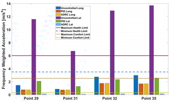
Figure 20.
Frequency-weighted accelerations for the uncontrolled, PID- and ADRC-controlled UAT operating under south wind direction at reduced cruise speed.

Figure 21.
Frequency-weighted accelerations for the uncontrolled, PID- and ADRC-controlled UAT operating under west-south-west wind direction at reduced cruise speed.
Figure 20 and Figure 21 show that at the lower cruise speed, all of the uncontrolled frequency-weighted RMS accelerations increased. The acceleration response of the PID-controlled UAT also increased, whereas that of the ADRC-controlled unit remained practically unchanged. This demonstrates the performance benefits of the ADRC flight controller design over that of the classical PID. Expectedly, the controlled longitudinal results show a trend similar to the one observed for the higher cruise speed in Figure 18 and Figure 19.
5. Discussion
The results presented in the previous section demonstrate the ability of the ADRC flight controller to outperform a PID flight controller when subjected to experimentally-derived urban airflow disturbances. It was shown that without suitable control, high accelerations can be experienced that can reach passenger discomfort levels and can potentially produce acceleration levels that are dangerous when gauged against the ISO 2631 limits. When the controllers were compared under the UAT trimmed condition for which the controllers were not originally tuned, which is the lower cruise speed in this case, the ADRC flight controller displayed a suitable lateral response whereas the PID controller exhibited a degradation of its lateral control performance. The longitudinal performance for both controllers was similar, which is attributed to the common single-channel pitch control, as discussed above. This will be addressed in future research.
Figure 18 and Figure 19 also demonstrate the potential for certain areas of the urban environment to experience higher levels of turbulence that can affect the accelerations, and hence comfort levels, experienced by a UAT. This is exemplified by data point 30 for the west-south-west wind direction and points 29, 32, and 35 for the south wind direction. This could indicate the presence of red zones [51] when it comes to safe operations of UAT. More locations in the urban environment should be investigated in future research to identify potential red zones.
The traditional linear flight dynamics model developed did not include aero-servo dynamics. Future investigations will include aeroservoelastic effects, unsteady aerodynamics and plant nonlinearities to better assess the full potential of ADRC for UAM. Furthermore, the effect of noisy Inertial Motion Units (IMUs) signals on the ADRC for UAM is currently being investigated.
6. Conclusions
A linearized flight dynamics model for a generic UAT was developed based on the Bell Nexus 4EX. Two inner-loop autopilot control algorithms were designed using PID and ADRC control laws to maintain the trimmed condition of the aircraft. Experimentally-collected urban airflow data were used to synthesize simplified airflow disturbances encountered by the UAT in flight. The acceleration responses of the uncontrolled UAT and of the PID- and ADRC-controlled unit were assessed and compared to the acceleration limits stated in the ISO 2631 standard [32].
It was observed that without control, a UAT could experience accelerations that are harmful to passengers. With the use of basic PID control, the accelerations can be reduced to levels that are not harmful but within the range of passenger discomfort levels. The ADRC flight controller was able to further reduce the lateral accelerations to below the minimum discomfort levels. With the data points that were used to create the urban airflow disturbances, it was observed that certain locations in the urban airspace may experience higher turbulence regardless of incoming wind direction, thereby indicating the presence of red zones [51]. The red zones could be different for various types of operations, such as organ delivery, light cargo, or passenger transportation.
Within the framework of the linear flight dynamics modelling presented herein, the performance of the ADRC was found to exceed the performance of the classical PID control in the lateral direction. The similar performance demonstrated between the two controllers in the longitudinal direction is attributed to the choice of longitudinal feedback control design. It was also found that ADRC could be tuned through similar qualitative methods that work well for PID and yet retains the ability to handle more complex non-linear systems. Future investigations will examine the performance of the controllers when nonlinear effects, such as control surface backlash and nonlinear aerodynamics, are included in the flight dynamics model. In addition, more complex and representative flow fields will be used to generate the wind disturbance in the model. Non-linear aerodynamics will have a significant effect when the UAT is operating at lower airspeeds upon approaching to land, during take-off, and when transitioning to the cruise phase. These phases of operation of the UAT will be the subject of future investigations.
The insights and the controllers’ gain-tuning implementation presented herein will provide the launch pad for these future investigations. The autopilot should also be extended to include the outer-loop control and to compare the performance of each controller when changing the set-point, which will enable the investigation of UAT navigation in an urban airflow environment. The current and planned future investigations should provide further insights into UAM and aid manufacturers and certification authorities in establishing more rigorous regulations and safety measures.
Author Contributions
Conceptualization, R.G.M., F.K., A.S.W. and G.L.L.; methodology, R.G.M.; software, R.G.M.; validation, R.G.M.; formal analysis, R.G.M.; investigation, R.G.M.; resources, R.G.M.; data curation, R.G.M.; writing—original draft preparation, R.G.M.; writing—review and editing, R.G.M., F.K., A.S.W. and G.L.L.; visualization, R.G.M.; supervision, F.K., A.S.W. and G.L.L.; project administration, R.G.M.; funding acquisition, R.G.M., F.K. and A.S.W. All authors have read and agreed to the published version of the manuscript.
Funding
This research received no external funding.
Data Availability Statement
Data are contained within the article.
Acknowledgments
I would like to acknowledge the NRC, NSERC, and Carleton University for their financial support which allowed for this investigation and my supervisors for their tireless support of this work. I would also like to acknowledge Maryam Al Labbad for her assistance in working with the urban airflow data and Tariq Maksoud for his assistance in tuning the ADRC flight controller.
Conflicts of Interest
Author Guy L. Larose was employed by the company Rowan Williams Davies & Irwin Inc. The remaining authors declare that the research was conducted in the absence of any commercial or financial relationships that could be construed as a potential conflict of interest.
Abbreviations
The following abbreviations are used in this manuscript:
| AAM | Advanced Air Mobility |
| ADRC | Active Disturbance Rejection Control |
| ESO | Extended State Observer |
| IMUs | Inertial Measurement Units |
| PSD | Power Spectral Density |
| RPAS | Remotely Piloted Aircraft Systems |
| SAS | Stability Augmentation System |
| STOL | Short Take-off and Landing |
| UAM | Urban Air Mobility |
| UAT | Urban Air Taxi |
| VTOL | Vertical Take-off and Landing |
Appendix A
Appendix A.1
The state space matrices in this section are for the original trimmed cruise conditions.
Appendix A.2
The state space matrices in this section are for the reduced speed trimmed cruise conditions of 120 mph with 10 degrees of flaps.
Appendix A.3
This section provides the estimated stability derivatives.
Table A1.
Longitudinal non-dimensional stability derivatives.
Table A1.
Longitudinal non-dimensional stability derivatives.
| u | −0.5028 | 0 | 0 |
| 0.8752 | −6.8307 | −1.0246 | |
| q | 0 | −25.7177 | −56.7287 |
| 0 | 0 | 0 |
Table A2.
Lateral non-dimensional stability derivatives.
Table A2.
Lateral non-dimensional stability derivatives.
| −0.4264 | −0.0587 | 0.1623 | |
| p | −0.1173 | −1.1936 | −0.4050 |
| r | 0.3247 | 0.9255 | −0.1236 |
Appendix A.4
This section provides the estimated control derivatives.
Table A3.
Longitudinal and lateral non-dimensional control derivatives.
Table A3.
Longitudinal and lateral non-dimensional control derivatives.
| Longitudinal | Lateral | ||||
|---|---|---|---|---|---|
| Elevator | Aileron | Rudder | |||
| 0 | 0 | −0.8273 | |||
| −1.1270 | 0.6788 | −0.1138 | |||
| 2.3385 | 0 | 0.3150 | |||
Appendix B. Nomeclature
Note that the symbols are ordered as they appear in the paper.
| Notation | Description |
| Aircraft Model Symbols | |
| body frame x direction | |
| body frame y direction | |
| body frame z direction | |
| wing-body angle of attack | |
| mean aerodynamic chord | |
| h | percent location of the centre of gravity |
| percent location of the main wing neutral point | |
| percent location of the wing-body neutral point | |
| distance between the main wing and canard aerodynamic centres | |
| distance between centre of gravity and canard aerodynamic centre | |
| elevator deflection angle | |
| flap deflection angle | |
| b | span |
| S | planform area |
| mass moment of inertia about x principal axis | |
| mass moment of inertia about y principal axis | |
| mass moment of inertia about z principal axis | |
| m | mass |
| H | body height |
| W | body width |
| L | body length |
| two-dimensional lift-curve slope | |
| wing thickness ratio | |
| sweepback angle of the leading edge | |
| a | three-dimensional lift-curve slope |
| aspect ratio | |
| two-dimensional lift-curve slope of wing-body | |
| two-dimensional lift-curve slope of canard | |
| two-dimensional lift-curve slope of vertical tail surface | |
| three-dimensional lift-curve slope of wing-body | |
| three-dimensional lift-curve slope of canard | |
| three-dimensional lift-curve slope of wing-body vertical tail surface | |
| trimmed lift coefficient | |
| W | aircraft weight |
| air density | |
| V | airspeed |
| aerodynamic moment coefficient of the aircraft at zero lift | |
| overall lift coefficient with respect to change in angle of attack | |
| overall moment coefficient with respect to change in angle of attack | |
| change in the lift coefficient due to elevator deflection | |
| change the moment coefficient due to elevator deflection | |
| trimmed angle of attack | |
| trimmed elevator deflection angle | |
| planform area of the canard | |
| h | location of the centre of gravity as a percentage of the mean aerodynamic |
| chord of the wing | |
| location of the overall UAT neutral point as a percentage of the mean | |
| aerodynamic chord of the wing | |
| elevator effectiveness coefficient | |
| horizontal tail (canard) volume ratio relative to the aerodynamic centres of | |
| the canard and wing-body | |
| elevator deflection angle | |
| flap deflection angle | |
| angle of attack relative to the zero-lift line | |
| angle of attack relative to the body x-axis | |
| longitudinal static margin | |
| x direction force with respect to forward air speed | |
| x direction force with respect to vertical air speed | |
| g | gravitational acceleration constant |
| trimmed pitch angle | |
| z direction force with respect to forward air speed | |
| z direction force with respect to vertical air speed | |
| z direction force with respect to rate of change of vertical air speed | |
| z direction force with respect to pitch rate | |
| trimmed airspeed | |
| mass moment of inertia about body y axis | |
| pitching moment with respect to forward air speed | |
| pitching moment with respect to rate of change of vertical air speed | |
| pitching moment with respect to vertical air speed | |
| pitching moment with respect to pitch rate | |
| change in x direction force with respect to control surface deflections | |
| change in z direction force with respect to control surface deflections | |
| change in pitching moment with respect to control surface deflections | |
| y direction force with respect to lateral air speed | |
| y direction force with respect to roll rate | |
| y direction force with respect to yaw rate | |
| rolling moment with respect to lateral air speed | |
| rolling moment with respect to roll rate | |
| rolling moment with respect to yaw rate | |
| yawing moment with respect to lateral air speed | |
| yawing moment with respect to roll rate | |
| yawing moment with respect to yaw rate | |
| mass moment of inertia with respect to x direction stability axis | |
| mass moment of inertia with respect to z direction stability axis | |
| mass product of inertia with respect to x-z direction stability axes | |
| rate of change of state vector | |
| x | state vector |
| u | control input vector |
| A | state matrix |
| B | control matrix |
| disturbance effect state matrix | |
| eigenvalues | |
| I | identity matrix |
| damping ratio | |
| natural frequency | |
| Urban Airflow Disturbance Symbols | |
| turbulence intensity in u airspeed direction | |
| turbulence intensity in v airspeed direction | |
| turbulence intensity in w airspeed direction | |
| Fourier series magnitude at location a, for frequency component j | |
| PSD amplitude at location a, for frequency component j | |
| frequency spacing | |
| time domain wind disturbance signal at location a | |
| N | maximum number of frequency components |
| the N frequency components that are evenly spaced at a fixed | |
| frequency spacing | |
| t | time |
| phase angle for each frequency | |
| Controller Symbols | |
| e | feedback signal error |
| PID proportional gain | |
| PID integral gain | |
| PID derivative gain | |
| PID integration parameter | |
| ADRC ideal control signal | |
| ADRC controller tuning parameters | |
| ADRC feedback error | |
| ADRC feedback error derivative | |
| ADRC function parameters | |
| , , | ADRC state estimates |
| , , | ADRC observer gains |
| ADRC function tuning parameters | |
| ADRC controller parameter | |
| h | ADRC ESO tuning parameter |
| ADRC set point signals | |
References
- Hill, B.P.; DeCarme, D.; Metcalfe, M.; Griffin, C.; Wiggins, S.; Metts, C.; Bastedo, B.; Patterson, M.D.; Mendonca, N.L. UAM Vision Concept of Operations (ConOps) UAM Maturity Level (UML) 4—NASA Technical Reports Server (NTRS). 2020. Available online: https://ntrs.nasa.gov/citations/20205011091 (accessed on 5 September 2023).
- UN. State of World Population 2007; United Nations Population Fund: New York, NY, USA, 2007. [Google Scholar] [CrossRef]
- Deschamps, T. Toronto Hospitals, Quebec Company Behind World’s First Delivery of Lungs by Drone. 2021. Available online: https://www.ctvnews.ca/sci-tech/toronto-hospitals-quebec-company-behind-world-s-first-delivery-of-lungs-by-drone-1.5619862 (accessed on 27 October 2023).
- Isik, O.K.; Hong, J.; Petrunin, I.; Tsourdos, A. Integrity analysis for GPS-based navigation of UAVs in urban environment. Robotics 2020, 9, 66. [Google Scholar] [CrossRef]
- Al Haddad, C.; Chaniotakis, E.; Straubinger, A.; Plötner, K.; Antoniou, C. Factors affecting the adoption and use of urban air mobility. Transp. Res. Part Policy Pract. 2020, 132, 696–712. [Google Scholar] [CrossRef]
- Yang, X.; Wei, P. Autonomous on-demand free flight operations in urban air mobility using Monte Carlo tree search. In Proceedings of the International Conference on Research in Air Transportation (ICRAT), Barcelona, Spain, 26–29 June 2018. [Google Scholar]
- Cotton, W.B.; Wing, D.J. Airborne trajectory management for urban air mobility. In Proceedings of the 2018 Aviation Technology, Integration, and Operations Conference, Atlanta, GA, USA, 25–29 June 2018; p. 3674. [Google Scholar]
- Adkins, K.A. Urban flow and small unmanned aerial system operations in the built environment. Int. J. Aviat. Aeronaut. Aerosp. 2019, 6, 10. [Google Scholar] [CrossRef]
- Archdeacon, J.L.; Iwai, N. Aerospace Cognitive Engineering Laboratory (ACELAB) Simulator for Urban Air Mobility (UAM) Research and Development. In Proceedings of the AIAA Aviation 2020 Forum, Virtual, 15–19 June 2020; p. 3187. [Google Scholar]
- Al Labbad, M.; Wall, A.; Larose, G.L.; Khouli, F.; Barber, H. Experimental investigations into the effect of urban airflow characteristics on urban air mobility applications. J. Wind. Eng. Ind. Aerodyn. 2022, 229, 105126. [Google Scholar] [CrossRef]
- FAA. Urban Air Mobility (UAM) Concept of Operations Version 2.0; Technical Report; FAA: Washington, DC, USA, 2023. [Google Scholar]
- Bassey, R. Engineering Brief No. 105, Vertiport Design; Technical Report; FAA: Washington, DC, USA, 2022. [Google Scholar]
- Kadhiresan, A.R.; Duffy, M.J. Conceptual Design and Mission Analysis for eVTOL Urban Air Mobility Flight Vehicle Configurations. In Proceedings of the AIAA Aviation 2019 Forum, Dallas, TX, USA, 17–21 June 2019. [Google Scholar] [CrossRef]
- Rostami, M.; Bardin, J.; Neufeld, D.; Chung, J. EVTOL Tilt-Wing Aircraft Design under Uncertainty Using a Multidisciplinary Possibilistic Approach. Aerospace 2023, 10, 718. [Google Scholar] [CrossRef]
- Brown, A.; Garcia, R. Concepts and Validation of a Small-Scale Rotorcraft Proportional Integral Derivative (PID) Controller in a Unique Simulation Environment. J. Intell. Robot. Syst. 2009, 54, 511–532. [Google Scholar] [CrossRef]
- Rostami, M.; Chung, J.; Park, H.U. Design optimization of multi-objective proportional-integral-derivative controllers for enhanced handling quality of a twin-engine, propeller-driven airplane. Adv. Mech. Eng. 2020, 12, 1687814020923178. [Google Scholar] [CrossRef]
- Yilmaz, E.; Warren, M.; German, B. Energy and landing accuracy considerations for urban air mobility vertiport approach surfaces. In Proceedings of the AIAA Aviation 2019 Forum, Dallas, TX, USA, 17–21 June 2019; p. 3122. [Google Scholar]
- Waslander, S.; Wang, C. Wind disturbance estimation and rejection for quadrotor position control. In Proceedings of the AIAA Infotech@Aerospace Conference, Seattle, WA, USA, 6–9 April 2009; p. 1983. [Google Scholar]
- Horn, J.; Cooper, J.; Schierman, J.; Sparbanie, S. Adaptive Gust Alleviation for a Tilt-Rotor UAV Operating in Turbulent Airwakes. In Proceedings of the AIAA Guidance, Navigation and Control Conference and Exhibit, Honolulu, HI, USA, 18–21 August 2008; p. 6514. [Google Scholar]
- Fezans, N.; Joos, H.D.; Deiler, C. Gust load alleviation for a long-range aircraft with and without anticipation. CEAS Aeronaut. J. 2019, 10, 1033–1057. [Google Scholar] [CrossRef]
- Giesseler, H.G.; Kopf, M.; Varutti, P.; Faulwasser, T.; Findeisen, R. Model Predictive Control for Gust Load Alleviation. IFAC Proc. Vol. 2012, 45, 27–32. [Google Scholar] [CrossRef]
- Zhao, Y.; Yue, C.; Hu, H. Gust Load Alleviation on a Large Transport Airplane. J. Aircr. 2016, 53, 1932–1946. [Google Scholar] [CrossRef]
- Li, Y.; Qin, N. A Review of Flow Control for Gust Load Alleviation. Appl. Sci. 2022, 12, 10537. [Google Scholar] [CrossRef]
- Frost, S.; Taylor, B.; Bodson, M. Investigation of Optimal Control Allocation for Gust Load Alleviation in Flight Control. In Proceedings of the AIAA Atmospheric Flight Mechanics Conference, American Institute of Aeronautics and Astronautics, Minneapolis, MN, USA, 13–16 August 2012. [Google Scholar] [CrossRef]
- Li, Y.; Qin, N. Airfoil gust load alleviation by circulation control. Aerosp. Sci. Technol. 2020, 98, 105622. [Google Scholar] [CrossRef]
- Guo, S.; Monteros, J.D.L.; Liu, Y. Gust Alleviation of a Large Aircraft with a Passive Twist Wingtip. Aerospace 2015, 2, 135–154. [Google Scholar] [CrossRef]
- Raza, S.A.; Etele, J. Autonomous Position Control Analysis of Quadrotor Flight in Urban Wind Gust Conditions. In Proceedings of the AIAA Guidance, Navigation, and Control Conference, San Diego, CA, USA, 4–8 January 2016. [Google Scholar] [CrossRef]
- Su, W.; Qu, S.; Zhu, G.G.; Swei, S.S.M.; Hashimoto, M.; Zeng, T. A control-oriented dynamic model of tiltrotor aircraft for urban air mobility. In Proceedings of the AIAA Scitech 2021 Forum, Virtual, 19–21 January 2021; p. 0091. [Google Scholar]
- Lombaerts, T.; Kaneshige, J.; Schuet, S.; Hardy, G.; Aponso, B.L.; Shish, K.H. Nonlinear dynamic inversion based attitude control for a hovering quad tiltrotor eVTOL vehicle. In Proceedings of the AIAA Scitech 2019 Forum, San Diego, CA, USA, 7–11 January 2019; p. 0134. [Google Scholar]
- Withrow-Maser, S.; Aires, J.; Ruan, A.; Malpica, C.; Schuet, S. Evaluation of Heave Disturbance Rejection and Control Response Criteria on the Handling Qualities Evaluation of Urban Air Mobility (UAM) eVTOL Quadrotors Using the Vertical Motion Simulator. In Proceedings of the VFS Aeromechanics for Advanced Vertical Flight Technical Meeting, San Jose, CA, USA, 25–27 January 2022. [Google Scholar]
- Gao, Z. Active disturbance rejection control: A paradigm shift in feedback control system design. In Proceedings of the 2006 American Control Conference, Minneapolis, MN, USA, 14–16 June 2006; IEEE: New York, NY, USA, 2006; p. 7. [Google Scholar]
- ISO 2631-1:1997; Mechanical Vibration and Shock—Evaluation of Human Exposure to Whole-Body Vibration—Part 1: General Requirements. Standard International Organization for Standardization: Geneva, Switzerland, 1997.
- Liu, Y. Study on the vibrational comfort of aircraft in formation flight. Aircr. Eng. Aerosp. Technol. 2020, 92, 1307–1316. [Google Scholar] [CrossRef]
- Kubica, F.; Madelaine, B. Passenger comfort improvement by integrated control law design. In Proceedings of the RTO AVT Specialists’ Meeting on “Structural Aspects of Flexible Aircraft Control”, Ottawa, ON, Canada, 18–20 October 1999. [Google Scholar]
- Hanson, C.E.; Andrade, S.; Pahle, J. Experimental Measurements of Passenger Ride Quality During Aircraft Wake Surfing. In Proceedings of the 2018 Atmospheric Flight Mechanics Conference, American Institute of Aeronautics and Astronautics, Atlanta, GA, USA, 25–29 June 2018. [Google Scholar] [CrossRef]
- Selič, V. Human Body Vibration Measurements on a Motorbike. 2023. Available online: https://dewesoft.com/blog/human-body-vibration-measurements-on-a-motorbike (accessed on 18 January 2024).
- Cook, M.V. Flight Dynamics Principles [a Linear Systems Approach to Aircraft Stability and Control], 2nd ed.; Butterworth-Heinemann/Elsevier: Oxford, UK, 2007. [Google Scholar]
- Joby Aviation. All Electric Air Mobility. 2021. Available online: https://www.jobyaviation.com/ (accessed on 6 July 2021).
- Lilium. Lilium. 2022. Available online: https://lilium.com/ (accessed on 8 February 2022).
- Parsons, D. City Airbus eVTOL Prototype Makes First Flight in Germany. 2019. Available online: https://www.aviationtoday.com/2019/05/06/city-airbus-evtol-prototype-makes-first-flight-germany/ (accessed on 7 November 2023).
- Volocopter. We Bring Urban Air Mobility to Your Life. 2021. Available online: https://www.volocopter.com/ (accessed on 6 July 2021).
- Electric VTOL News. Bell Nexus 4EX (Concept Design). Available online: https://evtol.news/bell-nexus-4ex/ (accessed on 27 October 2023).
- Bell Textron, Inc. Bell Boeing V-22 Osprey. Available online: https://www.bellflight.com/products/bell-boeing-v-22 (accessed on 7 November 2023).
- Bell Textron, Inc. Vintage Bell: The Bell X-22 Aircraft. 2020. Available online: https://news.bellflight.com/en-US/188762-vintage-bell-the-bell-x-22-aircraft (accessed on 7 November 2023).
- Johnson, O. Bell Unveils Electric Four-Ducted Nexus 4EX at CES 2020. 2020. Available online: https://verticalmag.com/news/bell-unveils-electric-four-ducted-nexus-4ex-at-ces-2020/ (accessed on 6 July 2021).
- Roskam, J. Airplane Design—Part V: Component Weight Estiomation; Design, Analysis and Research Corporation (DARcorporation): Lawrence, KS, USA, 2018. [Google Scholar]
- Hibbeler, R.C. Engineering Mechanics: Dynamics; Pearson Educación: London, UK, 2004. [Google Scholar]
- Etkin, B.; Reid, L.D. Dynamics of Flight: Stability and Control; Wiley: New York, NY, USA, 1996. [Google Scholar]
- Transport Canada. Airworthiness Manual Chapter 523 Preamble—Canadian Aviation Regulations (CARs). Available online: https://tc.canada.ca/en/corporate-services/acts-regulations/list-regulations/canadian-aviation-regulations-sor-96-433/standards/airworthiness-manual-chapter-523-normal-category-aeroplanes/airworthiness-manual-chapter-523-preamble-canadian-aviation-regulations-cars (accessed on 21 October 2021).
- Specification, M. Flying Qualities of Piloted Airplanes; Technical Report; MIL-F-8785C. 1980. Available online: https://www.abbottaerospace.com/downloads/mil-f-8785c-flying-qualities-of-piloted-airplanes/ (accessed on 22 November 2023).
- Al Labbad, M. The Effects of Urban Settings on Airflow Characterisitcs for Urban Air Mobility Applications. Master’s Thesis, Carleton University, Ottawa, ON, Canada, 2021. [Google Scholar]
- Wall, A.; Zan, S.; Langlois, R.; Afagh, F.F. Correlated turbulence modelling: An advancing Fourier series method. J. Wind. Eng. Ind. Aerodyn. 2013, 123, 155–162. [Google Scholar] [CrossRef]
- Han, J. From PID to active disturbance rejection control. IEEE Trans. Ind. Electron. 2009, 56, 900–906. [Google Scholar] [CrossRef]
Disclaimer/Publisher’s Note: The statements, opinions and data contained in all publications are solely those of the individual author(s) and contributor(s) and not of MDPI and/or the editor(s). MDPI and/or the editor(s) disclaim responsibility for any injury to people or property resulting from any ideas, methods, instructions or products referred to in the content. |
© 2024 by the authors. Licensee MDPI, Basel, Switzerland. This article is an open access article distributed under the terms and conditions of the Creative Commons Attribution (CC BY) license (https://creativecommons.org/licenses/by/4.0/).