Abstract
In this paper, a deep learning model trained to generate well-posed pressure distributions at transonic speeds is coupled by the efficient global optimization (EGO) algorithm to speed up the inverse design process for transonic airfoils. First, the Wasserstein generative adversarial network (WGAN) is trained to generate well-posed pressure distributions at transonic speeds. Then, the EGO algorithm is used to pick up a pressure distribution in WGAN by solving the associated optimization problem defined for matching the prescribed pressure features, such as the suction peak and the shock-wave position. Finally, a deep convolutional neural network (DCNN) for nonlinear mapping is adopted to obtain the corresponding airfoil shape. Several cases with prescribed pressure features were performed to verify the feasibility and efficiency of the proposed method. Test cases indicate that the airfoil shape with the desired pressure distribution can be found in around one minute using a desktop computer with an Intel i5-9300H CPU.
1. Introduction
Airfoils play a critical role in designing the aerodynamic shapes of air vehicles, gas turbines and wind turbines. They can be designed by either forward optimization design methods or inverse design methods. Forward optimization design requires a large number of CFD calculations and, therefore, consumes excessive resources. On the other hand, using the traditional airfoil inverse design is still time-consuming, due to the fact that the airfoil shape is adjusted to produce a prescribed pressure distribution by using a CFD-based optimization algorithm. In a practical preliminary design, it is highly desirable to find a reasonable airfoil design in minutes by using a desktop computer. Thus, a fast design method for airfoils is of practical significance.
There are already several inverse design methods that can reduce the design cost by mapping the pressure distribution to the geometry. For example, Bui-Thanh et al. [1] obtained a mapping relation between the pressure distribution and the airfoil geometry by using the proper orthogonal decomposition to reduce the dimensionality of data. Sekar et al. [2] proposed a deep convolutional neural network to quickly obtain geometric shapes from pressure distributions. However, these methods cannot directly specify the key features of pressure distributions, such as the suction peak and the shock-wave position, which are believed to be important for airfoil design at transonic speeds.
Recently, the generative model in deep learning was thought to be able to address this issue. This game-minded model can learn from existing datasets and generate new data consistent with the training data. Various generative models have been widely applied to speed up aerodynamic shape optimization. For instance, generative models are already used for airfoil shape parameterizations. Li et al. [3,4] used the generative adversarial network (GAN) proposed by Goodfellow et al. [5] to learn from the UIUC airfoil dataset and trained a discriminative model that can filter out abnormal airfoil geometries, thus greatly accelerating the aerodynamic optimization process. Chen et al. [6,7] used GAN to reduce the number of design variables, resulting in a great increase in design efficiency. Du et al. [8,9] proposed a new parameterization method by combining B-Spline and GAN to filter out abnormal geometries. This new parameterization method proved to be useful for rapid aerodynamic optimization. Yilmaz and German [10] and Achour et al. [11] have applied the generative model to associate the aerodynamic parameters with the airfoil geometry. In addition, generative models are also used for flow predictions. Wu et al. [12] proposed ffsGAN by combining the convolutional neural network and GAN and established a mapping relationship between supercritical airfoils and transonic flows to predict the flowfield of unseen airfoils. They further developed a data-enhanced generative model named daGAN [13] to overcome the sparsity of training data. The most attractive application of generative models is to generate reasonable aerodynamic characteristics by learning from a dataset. For example, Wang et al. [14] used CVAE-GAN to generate Mach number distributions with specified characteristics and then mapped them to airfoils. Lei et al. [15] developed a multistep inverse design process to design supercritical airfoils, where GAN was used to generate pictures containing physically existing pressure distributions.
However, the above-mentioned inverse design methods still require a relatively large time cost, which is not ideal for a fast preliminary design. Following the work by Lei et al. [15], this work aims to further increase the efficiency of airfoil inverse design at transonic speeds by combing the Wasserstein generative adversarial network (WGAN) [16] and the efficient global optimization (EGO) [17] algorithm. The WGAN is used to generate well-posed pressure distributions by learning from a dataset. Different from previous work, the pressure distribution curves are used as training data, resulting in a significant decrease in the number of latent variables required by WGAN. Then, the EGO algorithm is used to quickly find the target pressure distribution based on prescribed features including the suction peak, the shock-wave position and strength, and the pressure gradient. After finding the target pressure distribution, a deep convolutional neural network (DCNN) [18] is used to obtain the corresponding airfoil shape.
This paper first describes the flowchart of the inverse design process in Section 2, followed by the dataset preparation and the adopted deep learning models. Then, Section 3 presents the training process, followed by the results of WGAN models for generating pressure distributions and DCNN models for obtaining airfoil geometries. Section 4 presents inverse design results by the proposed method, followed by conclusions.
2. Methodology
The flowchart of the proposed method is presented in Figure 1. The airfoil inverse design based on deep learning models is used to quickly find an airfoil geometry with desired characteristics of pressure distribution. The design process can be expressed as follows: a Python script for the tasks of airfoil parameterization, mesh deformation and CFD calculations is first executed to collect the datasets containing a large number of airfoil geometries and the corresponding pressure distributions; then, these datasets are preprocessed for training deep learning models; after that, a WGAN model is trained to generate well-posed pressure distributions and the EGO algorithm is used to select the target pressure distribution that meets the requirements; finally, the pressure distribution is mapped to the airfoil geometry by the DCNN model.
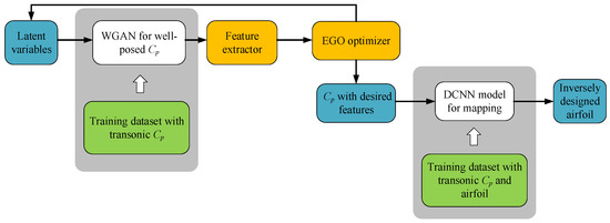
Figure 1.
Flowchart of the proposed method.
2.1. Dataset Preparation
Training datasets are obtained by a Python script. First, the Latin hypercube sampling (LHS) method is employed to generate multiple sampling points in the design space, which is defined by the class shape transformation (CST) [19] method where each airfoil surface is defined by
There, is the trailing-edge half-thickness and is a shape function defined as a linear combination of Bernstein polynomials of degree n:
In this work, the RAE2822 airfoil was used as the baseline airfoil. A CST method with n = 6 was used to deform the baseline airfoil shape. In order to generate sufficient and reasonable airfoils, the parameters in CST were constrained within the bounds of , resulting in design shapes shown in Figure 2. In total, 1000 airfoils were collected.
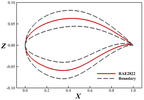
Figure 2.
Geometry of the baseline airfoil and the shape deformation boundary for dataset preparation.
The open-source CFD solver CFL3D [20,21] was used to solve the Reynolds-averaged Navier–Stokes (RANS) equations and obtain pressure distributions. The datasets used for network training were analyzed at flow conditions , and . As shown in Figure 3, the pressure distribution by CFD agrees well with the experimental result [22], indicating a satisfactory accuracy.
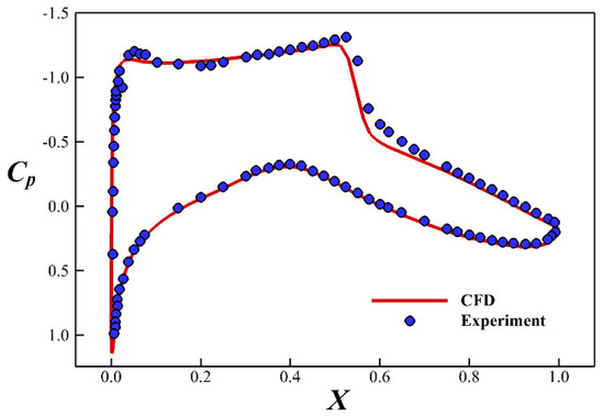
Figure 3.
Pressure distribution of CFD simulation and the experiment for RAE2822 baseline.
Each airfoil surface is represented by a total of 241 coordinate points (xi, zi) which are encoded as a tuple (x, z) and sorted in an anti-clockwise direction starting from the trailing edge. For CFD, the discrete surface is fitted by spline interpolation. The pressure coefficients of the corresponding coordinates are also stored as a tuple (x, Cp). In order to reduce the dimensionality of the input and output of the deep learning network to accelerate the training process, only z and Cp are allowed to be varied, whereas x coordinates are prescribed as
2.2. WGAN for Well-Posed Pressure Distributions
GAN adopts two adversarial models to learn from the training data. A generative model G is used to capture the real data distribution Preal and a discriminative model D is used to estimate the probability that a sample comes from the real data rather than from G. Models G and D are trained simultaneously to reach a Nash equilibrium, which is the optimal point for the loss function L in a two-player minimax game defined as
where and are the training sample and latent variables, respectively. is statistics expectation with respect to real data distribution Preal and distribution Pw of latent variables. By learning from Preal, G can produce similar data from only noise input.
GAN is known to be very unstable due to the mode collapse issue where the generative model can produce only a small portion of the trained distribution. The WGAN [16] has been proposed to address this issue. The Wasserstein distance function is used to quantify the distance between the real distribution and the generated distribution. WGAN optimizes the Jensen–Shannon (JS) divergence instead of the Kullback–Leibler (KL) divergence in order to overcome the collapse issue in the training process of the original GAN. Therefore, the loss function L of WGAN for synthesis and real data can be expressed as
where are neuronal parameters to be trained in D and is a weight-clipping boundary of D to enforce smoothness and stability.
The network architecture that consists of forward-propagation and back-propagation is adopted to implement WGAN as shown in Figure 4. Model G receives latent variables from the latent space, expressed in a standard normal distribution and generates Cp through an up-sampling process realized by transposed convolution layers. The Cp samples from real dataset and synthesized by G will be input into model D. Model D scores the samples to judge real or fake through a down-sampling process realized by convolution layers. The gradient of neuronal parameters with respect to loss function will be calculated through backpropagation. The parameters of the models will be updated by the RMSprop optimizer.
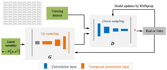
Figure 4.
Flowchart of the WGAN trained with a database.
In each epoch of training, model G tries to generate reasonable Cp to cheat model D, and model D is constantly updated to make correct judgments on real Cp and synthetic Cp. Finally, model D will be completely fooled by model G. The trained model G will be introduced into the optimization program as a well-posed Cp generator to find Cp with desired features.
2.3. Definition of Pressure Distribution
Generally, a practical transonic airfoil needs to satisfy multiple design objectives and constraints. It was found that the aerodynamic performances of an airfoil could be affected by the key features of its pressure distribution [23]. In order to obtain an airfoil with desired aerodynamic performances, the typical features of can be used as a merit function, which is subsequently optimized by the EGO optimizer to pick up the target pressure distribution in a design space spanned by the latent variables in the above-mentioned WGAN generative model G.
The features embedded in the pressure distributions can be of great value to aerodynamic design for transonic airfoils. Following the previous works [14,15], the features of the pressure distribution with a single shock are shown in Figure 5 and described as follows:
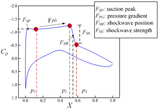
Figure 5.
Features of distribution.
Suction peak FSP: value at the point with the lowest pressure near the leading edge. The suction peak should not be too high to avoid an excessive shock intensity or unreasonable leading edge radius. In this work, the suction peak is calculated by choosing the minimal value of within the first 15% of the chord region resulting in
where .
Pressure gradient FPG: rise ratio of pressure platform in front of the shockwave. The pressure gradient has a great impact on the stability of the boundary layer. The natural laminar flow airfoil usually has a negative value to maximize the laminar flow area while the supercritical airfoil has a positive value to slowly recover pressure and avoid strong shock waves. It is defined as
where is the xi value at the start of the shock wave.
Shock-wave position FSW: value of the maximal rise ratio. Generally, a position near the middle chord is beneficial for drag reduction and drag divergence control. FSW is defined as:
where is the xi value at the end of the shock wave.
Shock-wave strength FSS: increase between two sides of the shock wave which directly indicates the shock drag performance of transonic airfoils:
Note that more complicated features can also be incorporated into this method to generate specific distributions for different aerodynamic design problems. This is different from the conditional generative model. The method based on feature extraction does not need to retrain the generative model.
2.4. DCNN Model for Airfoil Geometry
The nonlinear mapping of the pressure distribution to the airfoil shape is realized by a deep convolution neural network (DCNN), whose architecture is symbolically depicted in Figure 6. The mapping models are obtained by making the predicted output as close as possible to the ground truth.
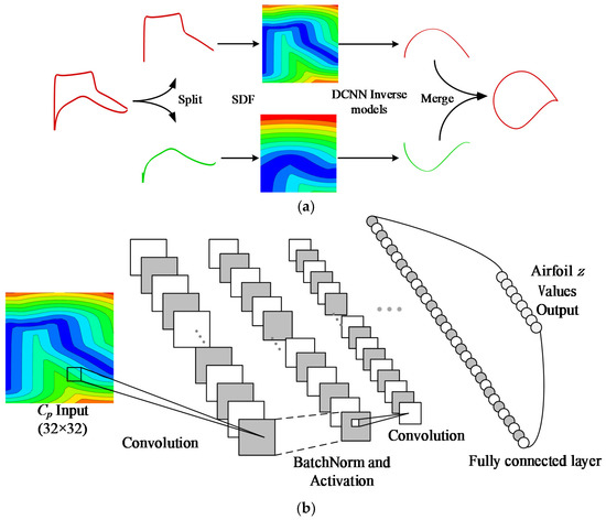
Figure 6.
Architecture of DCNN to generate airfoil shape from distribution: (a) Demonstration of airfoil geometry predicted by two independent DCNN models; (b) DCNN model for airfoil geometry mapping.
In order to improve the model accuracy, the upper and lower airfoil surfaces are trained by two independent DCNN models, respectively. The DCNN architecture consists of convolution layers, batch normalization layers and a fully connected layer. The inputs to the network are the pressure distributions in the form of a 32 × 32 2D matrix described below. Note that using structured matrixes in DCNN is similar to utilizing images as input, which can reduce the number of parameters in the network. The outputs of the network are z values representing the airfoil geometry.
A method based on the signed distance function (SDF) [24] is used to represent the pressure distribution. The combination of SDF and CNN can obtain smoother airfoil geometry than a multi-layer perceptron. Discrete pressure coefficient points will be fitted into a curve C by spline interpolation. The SDF at a point in the 2D matrix is defined as its minimum distance away from curve C. Its mathematical formula can be expressed as:
where determines whether the point is inside or outside the curve. Here because the curve C is not closed. The pressure distribution is represented by a 32 × 32 Cartesian grid within .
3. Model Training and Performance Analysis
In this section, the training processes of both WGAN and DCNN will be described, followed by their performance analysis. The open-source software PyTorch [25] is adopted for the following study.
3.1. Parameter Selection of WGAN
The architecture of the WGAN network is described in Table 1. The model G receives the latent variables from the latent space. Usually, a 100-dimensional latent space is considered to be big enough. In D, we use convolution layers (C layer) with a stride r = 2 instead of adding a pooling layer because it tends to improve the overall accuracy and stability. Similarly, the up-sampling in G is performed by using the transposed convolution layers (TC layer) with r = 2, rather than by adding an unpooling layer. The last layer of D is a full-connected layer (FC layer) to judge according to the characteristics. We chose ReLU and leakyReLU as activation functions (AF) of G and D, respectively, by considering the fact that these two functions have good stability during the training process.

Table 1.
Architecture details of model G and model D.
The kernel size Nsize and the filter depth Ndepth are two important parameters that influence the convergence and performance of WGAN. We conduct several tests to determine the proper values for these parameters. Figure 7 shows the convergence histories of the loss function and synthetic pressure distributions of generative models with different values of Nsize and Ndepth. The loss functions of model G and model D follow the description in the Equation (6). The kernel size Nsize is selected from and the filter depth Ndepth is selected from . The remaining parameters were determined by trial and error, which are listed as follows: the training epoch equals 500, the batch size equals to 64, the learning rate equals to 0.0001 for both G and D and the clipping weight of D equals to 0.01. It was found that the kernel size has a significant influence on the performance of WGAN. The generative model with Nsize < 5 fails to produce a smooth pressure distribution. Furthermore, increasing Nsize helps WGAN models to converge faster. The filter depth Ndepth should be greater than 5 to generate a reasonable distribution. According to our experiences, the model with Ndepth = 10 and Nsize = 7 was selected in this work.
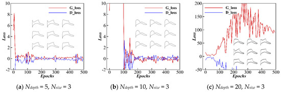
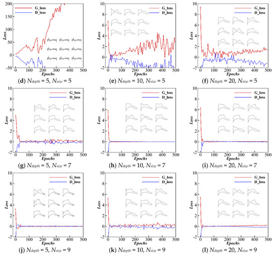
Figure 7.
Converge histories of G and D for different Ndepth and Nsize.
The maximum mean discrepancy (MMD) metric can be used to evaluate the diversity of synthetic pressure distributions by calculating the similarity between the real data and the generated data. A lower MMD means that the distribution of generated data is closer to that of real data. It is defined as:
where n and m are the numbers of real and generated samples. and are the ith Cp sample from a real dataset and generated dataset. and are the real and generated distribution, respectively, and is the kernel function with .
We studied the convergence of the latent space dimension (from 1 to 100) of latent variables based on the MMD scores. A total of 1000 synthetic pressure distributions generated by trained models were compared with the original training dataset. The results are listed in Table 2. It can be clearly seen that increasing the dimension of latent space results in a lower MMD score, which is desirable. The MMD score no longer decreases as the dimension of latent space reaches to 10, which is significantly smaller than that in the previous work [15]. The following study proceeds with a 10-dimensional latent space.
Table 2.
Convergence study of the latent space dimension.
3.2. Parameter Selection of DCNN
In the training process of DCNN, 80% of samples were used to train the network and the remaining 20% of samples were used to validate its performance. The number of layers, kernel size and choice of activation functions are often referred to as parameters needed to be selected before training. By trial and error, we designed five CNN models with different kernel sizes and filter depths. The comparison of the networks is given in Table 3. The other parameters were determined by setting the learning rate as 1.0 × 10⁻⁵, the batch size as 64 and the training epoch as 1250.
Table 3.
Kernel size, filter depth and neurons of DCNN models.
CNN training can be seen as an optimization problem, in which the parameters (weights and biases) of the network are updated using the backpropagation algorithm. The optimization involves minimizing a loss function that defines the deviation of a prediction and its true value. The mean square error (MSE) is used as the loss function defined as
where and are ith true z value and prediction of airfoil geometry, and m is the batch size during training.
Figure 8 shows the testing loss with different DCNN models. The performance of DCNN is insensitive to the kernel size and the number of layers. Furthermore, the performance of CNN5-3 with the medium kernel size and shallow layers is slightly better than that of the other models. Therefore, CNN5-3 will be used in the following study. Figure 9 shows the convergence history of the CNN5-3 model. After 1250 epochs, the loss function MSE drops by three orders of magnitude, indicating a reasonable convergence.
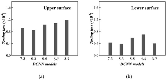
Figure 8.
Testing loss of DCNN model for (a) upper surface and (b) lower surface.
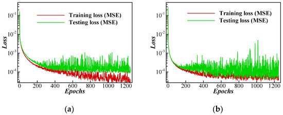
Figure 9.
Converge history of the loss function in CNN5-3 for (a) upper surface and (b) lower surface.
The absolute error is further used to assess the prediction accuracy of airfoil shape where n represents the total number of test samples. The result is shown in Figure 10. It can be seen that the error is below the tolerance requirement proposed by Sobieczky [26], which is 0.0007. It indicates that the designed DCNN model is capable of accurately generating the corresponding airfoil shape by a given pressure distribution.
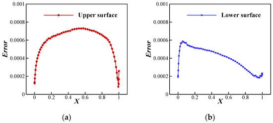
Figure 10.
Error distribution at the predicted points along the chord-wise direction of (a) upper surface and (b) lower surface.
Figure 11 shows the four predicted airfoils by DCNN. Although the pressure distributions have various suction peaks, pressure gradients, shock-wave positions and shock-wave strengths, DCNN can produce reliable airfoil predictions that are almost indistinguishable from the true airfoils.
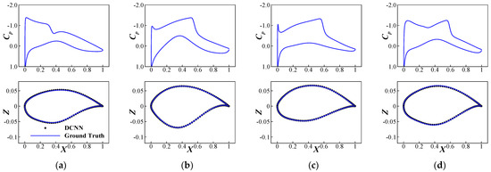
Figure 11.
Typical predicted results by DCNN from different pressure distributions: (a) test sample 1; (b) test sample 2; (c) test sample 3; (d) test sample 4.
4. Results and Discussions
This section will present the design results by using the above deep learning models. The calculations were conducted on a desktop computer with an Intel i5-9300H CPU.
4.1. Design for Various Features
The optimization problem for finding the target pressure distribution is defined as follows:
where , and are predetermined target features added as required. The design variables are the latent variables to model G of WGAN. This optimization problem is solved by the EGO optimizer.
Figure 12 shows four inverse design results with different FSP varying from −1.3 to −1.0 and FSW is fixed at the chord position of 0.5c where c represents the chord length. The target pressure distribution is found by the EGO optimizer and the airfoil shape is generated by the DCNN model. It can be seen that the desirable suction peak is well realized by the inverse design. Note that the FSP is defined as the minimal value of Cp in the first 15% chord region. Due to some defects in the geometry predicted by DCNN, such as insufficient smoothness and cross of trailing edge coordinates, the designed airfoil shape is fitted by a CST function, and then validated by the high-fidelity CFD simulation. The pressure distribution by WGAN shows good agreement with that by the CFD simulation. Figure 13 shows four inverse design results with different FSW varying from 0.44c to 0.56c where FSP is fixed as −1.2. It can be seen that the shock-wave position is changed as the prescribed value and the pressure distribution by WGAN is very close to that of the CFD simulation. Figure 14 shows the design results for different FPG varying from −0.8 to 0.4. It can be seen that the target pressure distribution is well realized by the inverse design and shows good agreement with that by the CFD simulation.
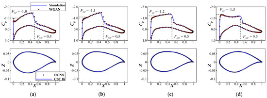
Figure 12.
Typical inverse design results produced by different suction peak features: (a) FSP = −1.0, FSW = 0.5; (b) FSP = −1.1, FSW = 0.5; (c) FSP = −1.2, FSW = 0.5; (d) FSP = −1.3, FSW = 0.5.
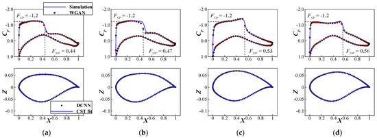
Figure 13.
Typical inverse design results produced by different shock-wave position features: (a) FSP = −1.2, FSW = 0.44; (b) FSP = −1.2, FSW = 0.47; (c) FSP = −1.2, FSW = 0.53; (d) FSP = −1.2, FSW = 0.56.
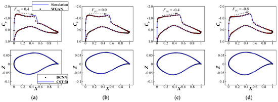
Figure 14.
Typical inverse design results produced by different pressure gradient features: (a) FPG = 0.4; (b) FPG = 0.0; (c) FPG = −0.4; (d) FPG = −0.8.
In summary, it can be concluded that the pressure distribution can be well designed according to the requirements by using the proposed inverse design method.
4.2. Design for Various Airfoils
This section will consider more practical airfoil design requirements. The optimization problem is defined as minimizing the shock-wave strength subject to a number of constraints according to the design requirements. The definition of the optimization problem is shown in Table 4, where c1 and c2 may be chosen based on design requirements.
Table 4.
Optimization problem statement for different inverse design requirements.
In total, four inverse design cases with different constraints were carried out. The convergence histories of the EGO optimizer are shown in Figure 15. It can be seen that the convergence results are obtained within 200 iterations. The inverse design results of DCNN are shown in Figure 16. The CFD simulation results of the inversely designed airfoils agree well with the target pressure distribution generated by WGAN. Interestingly, it can be observed that a more negative FPG requirement for natural laminar flow airfoils causes the optimizer to select a pressure distribution with a stronger shock wave, as shown by Design 3. Design 1 and Design 2 are close to the shape of a supercritical airfoil, whereas Design 3 and Design 4 are close to the shape of a transonic airfoil with natural laminar flow features.
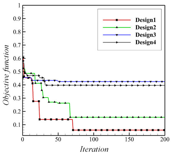
Figure 15.
Convergence history of the pressure distribution filtering process.
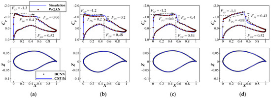
Figure 16.
Typical inverse design results produced by different constraint combinations: (a) Design 1: c1 = −1.3, c2 = 0.4; (b) Design 2: c1 = −1.2, c2 = 0.4; (c) Design 3: c1 = −1.2, c2 = 0.0; (d) Design 4: c1 = −1.1, c2 = 0.0.
Note that the time cost for each case is around one minute by assuming that the deep learning models are already available. It is believed that deep learning models can be easily trained by high-performance computers and stored in a database. Then, airfoils with various desired features can be found by a desktop computer in minutes.
5. Conclusions
A data-driven inverse design method has been developed for transonic airfoils. Deep learning models and the EGO algorithm have been combined to accelerate the design process for fast airfoil design. Each airfoil design has been completed in around one minute using a desktop computer with an Intel i5-9300H CPU.
Several test cases confirm the results in previous work. Various features of pressure distribution can be directly specified according to the design requirements and the target pressure distribution by the WGAN model shows good agreement with that of high-fidelity CFD simulation.
It has been found that using the pressure distribution curves as training data can significantly reduce the number of latent variables required by WGAN. A 10-dimensional latent space has been found to be enough for generating well-posed pressure distributions with sufficient accuracy, greatly reducing the time cost.
Author Contributions
Conceptualization, F.D.; methodology, J.Y.; software, J.Y.; validation, J.Y. and F.D.; formal analysis, J.Y.; investigation, J.Y.; resources, F.D.; data curation, J.Y.; writing—original draft preparation, F.D. and J.Y.; writing—review and editing, F.D.; visualization, J.Y.; supervision, F.D.; project administration, F.D.; funding acquisition, F.D. All authors have read and agreed to the published version of the manuscript.
Funding
This research was funded by the projects supported by National Natural Science Foundation of China (No. 12032011). This work was also supported by a project funded by the Priority Academic Program Development of Jiangsu Higher Education Institutions of China.
Institutional Review Board Statement
Not applicable.
Data Availability Statement
Not applicable.
Conflicts of Interest
The authors declare no conflict of interest.
Nomenclature
| Pressure coefficient | |
| Airfoil chord length | |
| D | Discriminative model |
| Dimension of latent variable | |
| G | Generative model |
| Loss function | |
| Freestream Mach number | |
| Reynolds number based on the chord length | |
| Sample from dataset | |
| Latent variable of WGAN | |
| normalized coordinates | |
| Tuple for storing coordinates | |
| Angle of attack | |
| MSE | Mean square error |
| SDF | Signed distance function |
References
- BuiThanh, T.; Damodaran, M.; Willcox, K. Aerodynamic Data Reconstruction and Inverse Design Using Proper Orthogonal Decomposition. AIAA J. 2004, 42, 1505–1516. [Google Scholar] [CrossRef]
- Sekar, V.; Zhang, M.; Shu, C.; Khoo, B.C. Inverse Design of Airfoil Using a Deep Convolutional Neural Network. AIAA J. 2019, 57, 993–1003. [Google Scholar] [CrossRef]
- Li, J.; Zhang, M.; Martins, J.; Shu, C. Efficient Aerodynamic Shape Optimization with Deep-Learning-Based Geometric Filtering. AIAA J. 2020, 58, 4243–4259. [Google Scholar] [CrossRef]
- Li, J.; Zhang, M. On Deep-Learning-Based Geometric Filtering in Aerodynamic Shape Optimization. Aerosp. Sci. Technol. 2021, 112, 106603. [Google Scholar] [CrossRef]
- Goodfellow, I.; Pouget-Abadie, J.; Mirza, M.; Xu, B.; Warde-Farley, D.; Ozair, S.; Courville, A.; Bengio, Y. Generative Adversarial Nets. In Proceedings of the Advances in Neural Information Processing Systems 27, Montreal, QC, Canada, 8–13 December 2014; pp. 2672–2680. [Google Scholar]
- Chen, W.; Chiu, K.; Fuge, M. Aerodynamic Design Optimization and Shape Exploration Using Generative Adversarial Networks. In Proceedings of the AIAA Scitech 2019 Forum, San Diego, CA, USA, 7–11 January 2019. [Google Scholar]
- Chen, W.; Chiu, K.; Fuge, M.D. Airfoil Design Parameterization and Optimization Using Bézier Generative Adversarial Networks. AIAA J. 2020, 58, 4723–4735. [Google Scholar] [CrossRef]
- Du, X.; He, P.; Martins, J. A B-Spline-Based Generative Adversarial Network Model for Fast Interactive Airfoil Aerodynamic Optimization. In Proceedings of the AIAA Scitech 2020 Forum, Orlando, FL, USA, 6–10 January 2020. [Google Scholar]
- Du, X.; He, P.; Martins, J. Rapid Airfoil Design Optimization via Neural Network-Based Parameterization and Surrogate Modeling. Aerosp. Sci. Technol. 2021, 113, 106701. [Google Scholar] [CrossRef]
- Yilmaz, E.; German, B. Conditional Generative Adversarial Network Framework for Airfoil Inverse Design. In AIAA Paper 2020-3185, Proceedings of the AIAA Aviation 2020 Forum, Virtual Event, 15–19 June 2020; American Institute of Aeronautics and Astronautics: Orlando, FL, USA, 2020. [Google Scholar]
- Achour, G.; Sung, W.J.; Pinon-Fischer, O.J.; Mavris, D.N. Development of a Conditional Generative Adversarial Network for Airfoil Shape Optimization. In AIAA Paper 2020-2261, Proceedings of the AIAA Scitech 2020 Forum, Orlando, FL, USA, 6–10 January 2020; American Institute of Aeronautics and Astronautics: Orlando, FL, USA, 2020. [Google Scholar]
- Wu, H.; Liu, X.; An, W.; Chen, S.; Lyu, H. A Deep Learning Approach for Efficiently and Accurately Evaluating the Flow Field of Supercritical Airfoils. Comput. Fluids 2019, 198, 104393. [Google Scholar] [CrossRef]
- Wu, H.; Liu, X.; An, W.; Lyu, H. A Generative Deep Learning Framework for Airfoil Flow Field Prediction with Sparse Data. Chin. J. Aeronaut. 2021, 35, 470–484. [Google Scholar] [CrossRef]
- Wang, J.; Li, R.; He, C.; Chen, H.; Cheng, R.; Zhai, C.; Zhang, M. An Inverse Design Method for Supercritical Airfoil Based on Conditional Generative Models. Chin. J. Aeronaut. 2022, 35, 62–74. [Google Scholar] [CrossRef]
- Lei, R.; Bai, J.; Wang, H.; Zhou, B.; Zhang, M. Deep Learning Based Multistage Method for Inverse Design of Supercritical Airfoil. Aerosp. Sci. Technol. 2021, 119, 107101. [Google Scholar] [CrossRef]
- Arjovsky, M.; Chintala, S.; Bottou, L. Wasserstein Generative Adversarial Networks. In Proceedings of the 34th International Conference on Machine Learning, Sydney, NSW, Australia, 6–11 August 2017; Volume 70, pp. 214–223. [Google Scholar]
- Jones, D.R.; Schonlau, M.; Welch, W.J. Efficient Global Optimization of Expensive Black-Box Functions. J. Glob. Optim. 1998, 13, 455–492. [Google Scholar] [CrossRef]
- Lecun, Y.; Bengio, Y.; Hinton, G. Deep Learning. Nature 2015, 521, 436. [Google Scholar] [CrossRef] [PubMed]
- Kuifan, B.M. Universal Parametric Geometry Representation Method. J. Aircr. 2008, 45, 142–158. [Google Scholar]
- Sclafani, A.J.; DeHaan, M.A.; Vassberg, J.C.; Rumsey, C.L.; Pulliam, T.H. Drag Prediction for the Common Research Model Using CFL3D and OVERFLOW. J. Aircr. 2014, 51, 1101–1117. [Google Scholar] [CrossRef]
- CFL3D. Available online: https://cfl3d.larc.nasa.gov/ (accessed on 19 November 2022).
- Cook, P.; Firmin, M.; Mcdonald, M. Aerofoil Rae2822: Pressure Distributions and Boundary Layer and Wake Measurements; AGARD AR 138; Royal Aircraft Establishment: Farnborough, UK, 1979.
- Run, Z.; Kai, W.; Yu, F.; Hai, X. Pressure Distibution Guided Supercritical Wing Optimization. Chin. J. Aeronaut. 2018, 31, 1842–1854. [Google Scholar]
- Guo, X.; Li, W.; Iorio, F. Convolutional Neural Networks for Steady Flow Approximation. In Proceedings of the 22nd ACM SIGKDD International Conference on Knowledge Discovery and Data Mining, San Francisco, CA, USA, 13–17 August 2016; pp. 481–490. [Google Scholar]
- PyTorch. Available online: https://github.com/Pytorch/Pytorch (accessed on 19 November 2022).
- Sobieczky, H. Parametric Airfoils and Wings. In Recent Development of Aerodynamic Design Methodologies. Notes on Numerical Fluid Mechanics (NNFM); Fujii, K., Dulikravich, G.S., Eds.; Vieweg + Teubner Verlag: Wiesbaden, Germany, 1999; pp. 71–87. ISBN 978-3-322-89954-5. [Google Scholar]
Disclaimer/Publisher’s Note: The statements, opinions and data contained in all publications are solely those of the individual author(s) and contributor(s) and not of MDPI and/or the editor(s). MDPI and/or the editor(s) disclaim responsibility for any injury to people or property resulting from any ideas, methods, instructions or products referred to in the content. |
© 2023 by the authors. Licensee MDPI, Basel, Switzerland. This article is an open access article distributed under the terms and conditions of the Creative Commons Attribution (CC BY) license (https://creativecommons.org/licenses/by/4.0/).