Article

Assessing Annual Actual Evapotranspiration Based on Climate, Topography and Soil in Natural and Agricultural Ecosystems

by
Kleoniki Demertzi
1,
Vassilios Pisinaras
2,
Emanuel Lekakis
3,
Evangelos Tziritis
2,
Konstantinos Babakos
2 and
Vassilis Aschonitis
2,*
1
Goulandris Natural History Museum, Greek Biotope/Wetland Centre, 57001 Thessaloniki, Greece
2
Hellenic Agricultural Organization-Demeter, Soil and Water Resources Institute, 57001 Thessaloniki, Greece
3
Agroapps P.C., 57001 Thessaloniki, Greece
*
Author to whom correspondence should be addressed.
Climate 2021, 9(2), 20; https://doi.org/10.3390/cli9020020
Submission received: 12 December 2020 / Revised: 13 January 2021 / Accepted: 18 January 2021 / Published: 21 January 2021
(This article belongs to the Special Issue Climate Ecosystems Nexus)

Abstract

:
Simple formulas for estimating annual actual evapotranspiration (AET) based on annual climate data are widely used in large scale applications. Such formulas do not have distinct compartments related to topography, soil and irrigation, and for this reason may be limited in basins with high slopes, where runoff is the dominant water balance component, and in basins where irrigated agriculture is dominant. Thus, a simplistic method for assessing AET in both natural ecosystems and agricultural systems considering the aforementioned elements is proposed in this study. The method solves AET through water balance based on a set of formulas that estimate runoff and percolation. These formulas are calibrated by the results of the deterministic hydrological model GLEAMS (Groundwater Loading Effects of Agricultural Management Systems) for a reference surface. The proposed methodology is applied to the country of Greece and compared with the widely used climate-based methods of Oldekop, Coutagne and Turk. The results show that the proposed methodology agrees very well with the method of Turk for the lowland regions but presents significant differences in places where runoff is expected to be very high (sloppy areas and areas of high rainfall, especially during December–February), suggesting that the proposed method performs better due to its runoff compartment. The method can also be applied in a single application considering irrigation only for the irrigated lands to more accurately estimate AET in basins with a high percentage of irrigated agriculture.

1. Introduction

Actual evapotranspiration is a crucial component of both water and energy balance, which plays a significant role in climate–soil–vegetation interactions [1,2]. It is an extremely complicated biophysical procedure since it is regulated by the combination of climate, soil, topography, vegetation type and density [3]. For this reason, its measurement is only feasible in small scale applications (e.g., by using weighing lysimeters) while it is practically and economically impossible over long periods of time in large scale applications [4]. The methods of estimating actual evapotranspiration are divided into plant physiological, micrometeorological and hydrological estimations depending on the purposes of the study [5]. In the case of large-scale applications (e.g., basin-scale and beyond), the problem of measuring evapotranspiration can be addressed by hydrological methods, which are based on various conceptual approaches such as assessing water balance components using physically-based hydrological models (e.g., SWAT, MIKE, etc.) [6,7], simplistic water balance models [3,8,9,10,11], or even more simple actual evapotranspiration formulas such as those of Oldekop [12], Coutagne [13], Turk [14], Bouchet [15,16], Budyko [17,18,19] or similar that provide relationships between annual actual evapotranspiration (AET), annual average precipitation and potential evapotranspiration or temperature. The Budyko concept, which in reality is the evolution of the Oldekop concept [20], is the most widely used method, and many efforts have been made to improve its proposed framework and to understand how climate and catchment characteristics regulate the long-term average water balance [21,22,23,24,25,26,27,28,29].
The aforementioned simplistic formulas of annual actual evapotranspiration do not take into account the following features that may lead to significant errors: (a) Surface runoff is the dominant water balance component in sloppy areas, leading to much lower rates of annual actual evapotranspiration; (b) In main river watersheds, irrigated agriculture dominates in the lowland areas, which leads to higher actual evapotranspiration rates even when annual rainfall is low; (c) Soil permeability regulates percolation and available water storage. In the Budyko-based formula of Fu [22], all the above features were included in one empirical coefficient, which was later expressed by Sun et al. [27] as a function of saturated hydraulic conductivity, rainfall intensity and water holding capacity of the underlying surface.
In another field of research related to the analysis of water and nitrogen losses by agricultural lands, a new methodology was developed by Aschonitis et al. [30,31] for estimating water losses by runoff and percolation from a reference surface, with or without irrigation. The specific method was a hybrid method because it was developed using the results of a large number of simulations made by a physically-based hydrological model in order to calibrate regression formulas able to estimate the annual rates of runoff and percolation separately. The aim of this study was to show that the specific concept and formulas could be used in a simplistic water balance approach in large-scale applications for assessing annual actual evapotranspiration of natural ecosystems but also to assess irrigated agricultural ecosystems considering easily obtained information about climate, soil, topography and irrigation. The specific concept was applied to the country of Greece and was compared with other simplistic climate-based formulas of actual evapotranspiration that do not require calibration [12,13,14].

2. Materials and Methods

2.1. Derivation of Actual Evapotranspiration and Comparison with Previous Methods

The proposed methodology for estimating actual evapotranspiration is based on the losses of water (LOSW) indices [30,31] that assess the intrinsic rates of annual water losses from surface runoff (LOSW-R) and percolation (LOSW-P) of a reference surface. According to the LOSW concept, a reference surface was set as a uniform surface of actively dense cover with clipped perennial grass, whose rates of evapotranspiration under non-water stress conditions were equivalent to the reference crop evapotranspiration of American Society of Civil Engineers (ASCE)-standardized/Food Agriculture Organization of the United Nations (FAO)-56 concept [32,33]. The LOSW-P and LOSW-R indices were calibrated based on the inputs and outputs of simulation scenarios performed by the Groundwater Loading Effects of Agricultural Management Systems (GLEAMS) model [34]. The simulations covered: (i) Different soils with respective hydraulic characteristics of the four hydrological soil types A, B, C and D of USDA–NRCS [35]; (ii) Different topography by using different slopes of grass surfaces using the curve number vs. the slope of the grass surface relationship of Getter et al. [36]; (iii) Different climate conditions from Greece, Italy and USA; (iv) Irrigation or non-irrigation conditions. Irrigation was applied automatically by the GLEAMS model when the soil moisture was falling to 20% of available soil moisture (ASM) in order to return it to 100% ASM corresponding to field capacity conditions. All scenarios were performed for the first 30 cm of the soil profile, which included the largest percentage of the rootzone. The results were used to develop and calibrate LOSW-P and LOSW-R, which describe annual percolation and surface runoff water losses, according to the following equations [29]:
L O S W - P   = 0.0941 K s   0.761 S L   +   0.4185 P     0.0487 E T o   +   0.0903 I R 2
L O S W - R =     0.0856 K s   +   1.8573 S L   +   0.9966 P   0.5612 E T o   +   0.2384 I R 2
where LOSW-P is intrinsic percolation water losses (mm year−1), LOSW-R is intrinsic runoff water losses (mm year−1), Ks is saturated hydraulic conductivity (mm day−1), SL is soil surface slope (%), P is annual precipitation (mm year−1), ETo is the annual reference evapotranspiration (mm year−1) and IR is the annual irrigation to cover the deficit of reference evapotranspiration (mm year−1). It has to be noted that when the formulas inside the brackets of Equations (2) and (3) lead to negative values, the value of LOSW-P and LOSW-R are set equal to 0.
The above equations can be used either for IR = 0 or IR ≠ 0. For the latter case, the annual irrigation IR for covering the deficit of annual reference evapotranspiration is calculated as follows [30]:
I R = 1 12 I R i   ,   where   I R i = E T o , i P i   when   E T o , i > P i   else   I R i = 0
where IR is the annual irrigation required for covering the deficit of annual reference evapotranspiration (mm year−1), IRi is monthly irrigation for covering the deficit of reference evapotranspiration of the month i (mm month−1), ETo,i is monthly reference evapotranspiration (mm month−1) (estimated in this study by FAO-56 method), Pi is monthly precipitation and i is the month. The use of larger IR values from the values of Equation (3) for over-irrigation analysis using Equations (1) and (2) is not indicated.
The main aspect of LOSW indices, which has not been analyzed in previous studies, is that they can be used for the estimation of the actual evapotranspiration of the reference surface, taking into consideration not only the climate but also soil and topography. Thus, a new approach for estimating actual evapotranspiration ETa is built based on LOSW indices as follows:
L O S W - E T = T W L O S W - P L O S W - R
where LOSW-ET is the actual evapotranspiration of the reference surface (mm year−1), TW is the total water inflow equal to P + IR, where IR = 0, or is equal to Equation (3). Equation (4) is built under the assumption of null annual change in soil moisture storage ΔS ≈ 0 among sequential years. For general applications of Equation (4) with IR ≠ 0 estimated by Equation (3), the use of filter (LOSW-ET) = ETo is suggested when (LOSW-ET) > ETo. In this study, this filter was not used in order to show the overall response of Equation (4) when IR ≠ 0.
In this study, the LOSW-ET method was compared with the widely known ETa methods of Oldekop [12], Coutagne [13] and Turk [14]. The Oldekop method equation is the following:
E T D = P 1 exp E T o / P
where ETD is the annual Oldekop actual evapotranspiration (mm year−1), P is the annual precipitation (mm year−1) and ETo is the annual reference/potential evapotranspiration (mm year−1).
The Coutagne method equation is the following:
E T C = P           for         P < L / 8 E T C = P 1 P / L     for       L / 8 P L / 2 E T C = 200 + 35 T         for       P > L / 2       where   L = 800 + 140 T
where ETC is the annual Coutagne actual evapotranspiration (mm year−1), P is the annual precipitation (mm year−1), T is mean annual temperature (°C) and L is the function of temperature (unitless).
The Turk method equation is the following:
E T T = P           for         P / L T 0.316 E T T = P / 0.9 + P L T 2 0.5     for     P / L T > 0.316 where   L T = 300 + 25 T + 0.05 T 2
where ETT is the annual Turk actual evapotranspiration (mm year−1), P is annual precipitation (mm year−1), T is mean annual temperature (°C) and LT is the function of temperature (unitless).
The ETo in Equations (1)–(5) was estimated using the ASCE-standardized method (former FAO-56) for short reference crop by the following function [2]:
E T o = 0.408 Δ R n G + γ u 2 e s e a C n T + 273.16 Δ + γ 1 + C d u 2                                            
where ETo is the reference crop evapotranspiration (mm d−1), Rn is net radiation at the crop surface (MJ m−2 d−1), u2 is mean daily wind speed at 2 m height (m s−1), T is the mean daily air temperature (°C), G is soil heat flux density at the soil surface (MJ m−2 d−1), es is the mean daily vapor pressure (kPa), ea is the mean daily actual vapor pressure (kPa), Δ is the slope of the saturation vapor pressure–temperature curve (kPa °C−1), γ is the psychrometric constant (kPa °C−1) and Cn and Cd are constants of 900 and 0.34, respectively.

2.2. Study Area and Data

The LOSW-ET methodology for estimating actual evapotranspiration and the comparison with the other methods of Oldekop, Coutagne and Turk was employed for the case of Greece. The analysis was based on climatic data, which were obtained from the following four databases:
  • The database of Hijmans et al. [36] provides gridded data of mean monthly precipitation P and mean monthly temperature T for the period 1950–2000 (WorldClim version 1.2) at 30 arc-sec (~1 × 1 km) spatial resolution. Their mean annual values are given in Figure 1a,b, respectively, and their frequency histograms in Figure 2a,b, respectively.
  • The database of Aschonitis et al. [37] (10.1594/PANGAEA.868808) provides gridded data of mean monthly reference evapotranspiration ETo (Equation (8)) of the period 1950–2000 at 30 arc-sec (~1 × 1 km) spatial resolution (Figure 1c) (this database is built using temperatures from the WorldClim version 1.2 database). Using the ETo (Figure 1c) and precipitation (Figure 1a) from the previous database, the irrigation map of the reference crop IR is built according to Equation (3) (Figure 1d). The frequency histograms of ETo and IR are given in Figure 2c,d, respectively.
  • The surface slope (Figure 1e) is obtained by the digital elevation model of GTOPO30 (pixel analysis of 30 arc-sec, ~1 × 1 km) as it is given by the USGS (United States Geological Survey). The frequency histogram of the slope is given in Figure 2e.
  • The European Soil Database (ESDB) provided by the European Commission Joint Research Centre [38,39] provides soil data (% sand, % silt, % clay, % gravel, % organic carbon) with spatial analysis (~1 × 1 km). These data are used to estimate the saturated hydraulic conductivity Ks according to the respective pedotransfer function (PTF) of Saxton and Rawls [40], taking into account the gravel and organic matter effect (Figure 1f). The frequency histogram of Ks is given in Figure 2f.

3. Results

Taking into account Equation (4) (for IR ≠ 0 and IR = 0), and Equations (5)–(7), the mean annual values of actual evapotranspiration based on LOSW-ET(IR ≠ 0), LOSW-ET(IR = 0), ETD, ETC, and ETT were estimated for the period 1950–2000 for the whole country of Greece (Figure 3a–e). The frequency histograms of their respective raster values are given in Figure 4a–e.
As ETD, ETC and ETT do not consider irrigation, they were compared with LOSW-ET(IR = 0) using pedotransfer. The comparison was made in two ways. The first way was based on 1:1 plots (Figure 5a–c) between LOSW-ET(IR = 0) vs. ETD, ETC and ETT, respectively. The 1:1 plots were built using 15% of all pixels after random selection and exclusion of those with Ks = 0 (rocky areas). Linear trend lines and Spearman rank correlations were also determined (the given in the respective 1:1 plots). The second way was based on calculating the D difference in mm per year between the raster values of LOSW-ET(IR = 0) and ETD, ETC and ETT, respectively. The D difference of ETD, ETC and ETT from LOSW-ET(IR = 0) is given in the maps of Figure 6a–c, respectively. The respective frequency histograms of D raster values are given in Figure 7a–c. In the maps of Figure 6, the class of −50 mm < D < 50 mm in the legends is considered the class where LOSW-ET(IR = 0) is in good agreement with the ETD, ETC and ETT methods because their mean annual difference is in the range of ~±10%.
Taking into account the results of the 1:1 plots (Figure 5), D maps (Figure 6) and their histograms (Figure 7), it was observed that the actual evapotranspiration of Oldekop ETD and Coutagne ETC showed significantly higher values using LOSW-ET(IR = 0). ETD provided 29% greater values, while ETC provided almost 50% greater values from LOSW-ET(IR = 0) at the country level.
On the other hand, the comparison between LOSW-ET(IR = 0) and the ETT of Turk showed not only a good agreement at the country level based on their mean values (~3.5% difference according to Figure 4b,e), but also a much better trend line and Spearman correlation (Figure 5c) compared to ETD and ETC. Further investigation of Figure 6c showed that 73% of the total country coverage had D values inside the range of ±50 mm that corresponded to ~±10% mean annual difference. This is an extremely important finding since it shows that at least one of the three older actual evapotranspiration methods (ETD, ETC, ETT) is in accordance with LOSW-ET(IR = 0). Combining the results of Figure 6c with the maps given in Figure 1, it can be observed that D deviates from the range of ±50 mm in regions where the surface slope is >10% and in regions where annual ETo is >1200 mm with P/LT ≥ 1.
LOSW-ET(IR ≠ 0) can only be compared with ETo as it describes the irrigated reference crop evapotranspiration, including the effect of soil, topography and soil moisture reduction between irrigation intervals (the last effect is embodied in the LOSW-ET formula through its calibration with GLEAMS results). The 1:1 plot between LOSW-ET(IR ≠ 0) and ETo is given in Figure 8. According to Figure 8, ETo is always larger using LOSW-ET(IR ≠ 0) (21% larger at country level based on Figure 4a and Figure 2c). The trend line and the Spearman correlation show a good correspondence between ETo and LOSW-ET(IR ≠ 0). The smaller values of LOSW-ET(IR ≠ 0) compared to ETo are absolutely justified by the effect of soil moisture reduction between the irrigation intervals used in GLEAMS model simulations (automated irrigation is applied when soil moisture reaches 20% of available water). This option of automatic irrigation is selected on purpose since it gives a more realistic reflection of the actual evapotranspiration of a reference crop under actual irrigated conditions and not theoretical conditions of constant soil moisture at field capacity. Thus, LOSW-ET(IR ≠ 0) is expected to always be lower than ETo because it does not consider constant soil moisture conditions at field capacity.

4. Discussion

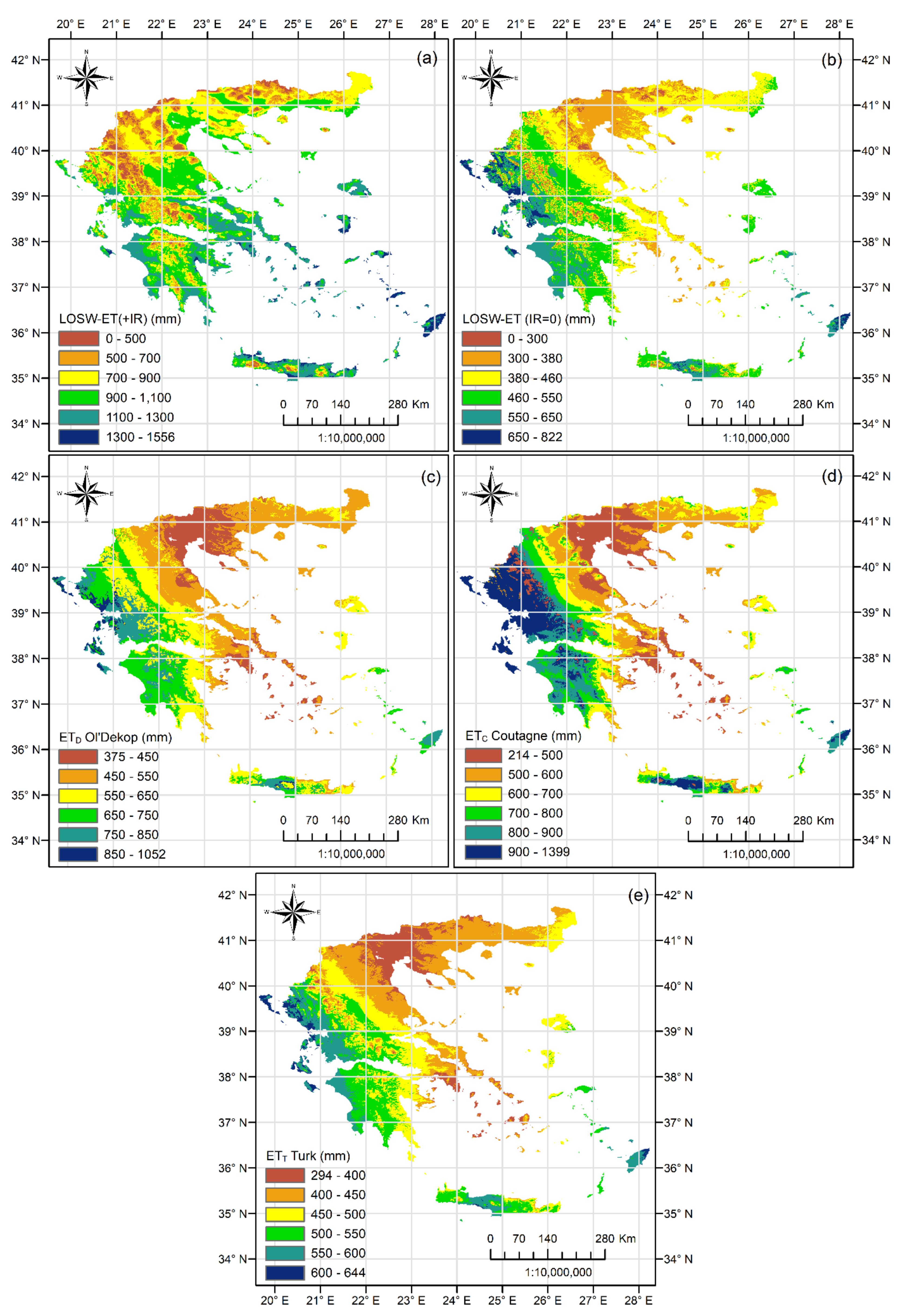
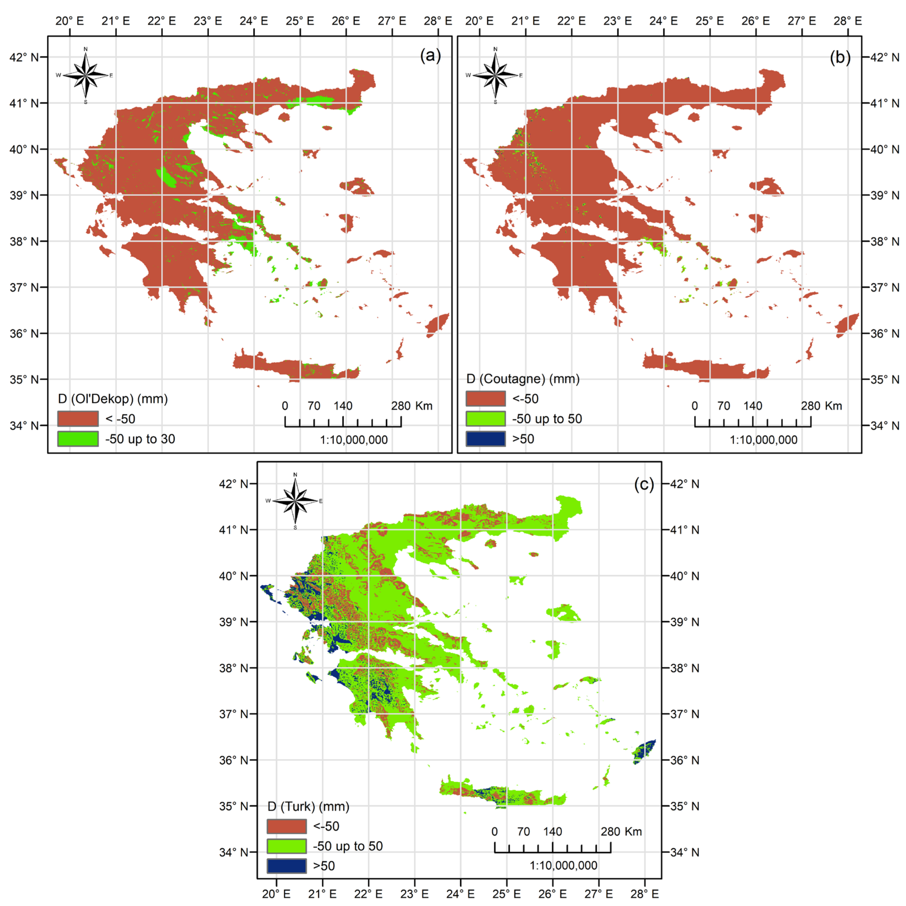
4.1. Differences between Actual Evapotranspiration Methods

As shown in Figure 3, Figure 4, Figure 5, Figure 6 and Figure 7, different methods of determining actual ET for IR = 0 can lead to extremely different results, which in many cases may seem unjustifiable. Before judging the validity of each method, it is crucial to understand that these differences may be the result of inevitable factors associated with the creator and the user, such as:
(a)
The creators used calibration data from different regions with extreme hydroclimatological differences that led to coefficients describing different attributes of hydroclimatic conditions.
(b)
Many of the methods were extremely old, and the accuracy and representativity of the data used for calibration were completely different when they were developed compared to the respective data provided nowadays. For example, the method of Oldekop is more than a century old, while most of the important methods, including Coutagne and Turk, are more than 50 years old.
(c)
The user may not apply the methods in the same way proposed by the creators. For example, the user may estimate the potential/reference evapotranspiration using a different method from the one used by the developer. For example, old methods had available data only for rainfall and temperature. Thus, potential evapotranspiration was mainly estimated using a temperature-based formula, e.g., the Thornthwaite method [41]. Nowadays, there is a vast amount of methods for estimating potential/reference evapotranspiration with limited or full data requirements depending on the data availability. This may be convenient but can also lead to differences not only between actual ET methods but also to differences between the results of the same actual ET method due to the use of a different ETo method.
The above may justify the observed differences between actual ET methods in this study, but it is also crucial to note that even similar results between two ET methods may be the result of a counterbalanced effect of the aforementioned factors.
Regarding the comparison between LOSW-ET(IR = 0) and ETT, it was observed that D deviated from the range of ±50 mm in regions where surface slope was >10%, regions where annual ETo was >1200 mm and P/LT ≥ 1 (Figure 6c). The negative values of D < −50 mm (i.e., LOSW-ET(IR = 0) < ETT) were mostly observed in sloppy regions, which was probably due to the runoff compartment Losw-R (Equation (2)) that pulled down actual evapotranspiration estimation by increasing runoff in higher slopes. The Ks parameter was not found to be a responsible driver of D deviation outside the range of ±50 mm, apart from cases where Ks ≈ 0 in very sloppy rocky areas where the high slope effect coincided with the Ks effect. The regions with positive D (LOSW-ET(IR = 0) > ETT) greater than 50 mm (Figure 6c) were regions that had the common characteristics of ETo > 1200 mm with P/LT ≥ 1, where almost half of annual precipitation and more than 10% of ETo occurred during December–February according to the cluster maps [42,43,44] that were developed using the same datasets. Thus, these regions tended to present higher actual evapotranspiration during winter compared to other regions in Greece due to higher P and ETo. If we assume that LOSW-ET(IR = 0) is more correct from ETT, then ETT will probably require an additional module for environments with P/LT ≥ 1; otherwise, LOSW-ET(IR = 0) needs improvements through recalibration with stations from the specific regions.

4.2. Inclusion or Noninclusion of Irrigation in Actual Evapotranspiration Methods

The application of the older actual evapotranspiration methods ETD, ETC and ETT raises concerns about their use in regions/basins with a large percentage coverage by irrigated crops since they do not consider irrigation. In this case, the concept of LOSW-ET provides the solution of the mixed model with the use of LOSW-ET(IR = 0) for natural areas and nonirrigated agricultural lands and the use of LOSW-ET(IR ≠ 0) for irrigated lands. The only additional input, which is required for the mixed LOSW-ET application, is a land cover map that can be obtained from various databases. An example of the mixed model use is given in Figure 9, where CORINE Land Cover 2018 was used to separate irrigated from nonirrigated lands in Greece (Figure 9a). Irrigated lands were considered in the LC (Land Cover) codes (212: permanently irrigated lands, 213: rice fields, 221: vineyards, 222: fruit trees and berry plantations), accounting for ~9.6% of the total country coverage. Other classes were not considered (e.g. 223: olive groves) because the irrigated portion was unknown. This was the same for the irrigated portion of vineyards (221). For this reason, the specific mixed model analysis is given as an example to stress the effect of a large proportion of irrigated lands on actual evapotranspiration. The pixels of irrigated lands obtained the values of LOSW-ET(IR ≠ 0) (Figure 3a), while the pixels of nonirrigated and natural lands obtained the values of LOSW-ET(IR = 0) (Figure 3b) in order to develop the final actual evapotranspiration map of the mixed LOSW-ET method (Figure 9b). The frequency histogram of mixed LOSW-ET raster values is given in Figure 9c. The mean annual value of the mixed LOSW-ET at the country level (Figure 9c) is about 10.7% larger than the respective LOSW-ET(IR = 0) (Figure 4b), highlighting a possible error in the calculation of actual evapotranspiration analogous to the portion of irrigated lands. If we consider that most of the applications are usually restricted in watersheds of significant rivers, which are hotspots of human presence and irrigated agriculture, then the expected errors of methods that do not consider the effect of irrigation is expected to be significant.
The use or non-use of the IR term in Equations (1) and (2) is regulated by the objectives of the user (e.g., for irrigated arable land or for nonirrigated land, and of course, for natural ecosystems). For the case of irrigated lands, LOSW-ET(IR ≠ 0) could further be adapted in order to improve the estimation of actual evapotranspiration. For example, if the types of irrigated crops in a region and their irrigation period is known, then IR can be calculated by Equation (3) only for the months of irrigation and also considering crop factors if they are available for the specific crops [45].

4.3. Possible Solutions for Validation

A basic limitation of the current study is the lack of validation of LOSW-ET with actual data. Since LOSW-ET is a method for estimating actual evapotranspiration, the most appropriate procedure would be to use actual evapotranspiration data. This option covering the full approach of LOSW-ET for various slopes and soil hydraulic properties under irrigation or no irrigation conditions is almost impossible from an experimental point of view since actual evapotranspiration is one of the most challenging parameters to measure, even with simple lysimeter conditions. An alternative way of validation would be to compare LOSW-ET results with the results of a distributed hydrological model (e.g., MIKE or SWAT) for a basin after being calibrated with actual values of runoff and if it is possible with additional values of percolation indirectly estimated by measurements of groundwater table variation.

5. Conclusions

The method of LOSW-ET extends the concept of actual evapotranspiration by including various dimensions of natural ecosystems such as soil and topography but also the dimension of irrigation in agricultural lands. The case of LOSW-ET(IR ≠ 0) also extends the concept of reference crop evapotranspiration ETo, which is basically a climatic parameter providing a more realistic estimation of the maximum evapotranspiration that can be achieved by taking the soil-topographic characteristics and the effect of soil moisture variation between realistic irrigations into consideration.
The overall approach, and especially in the case of mixed LOSW-ET, seems promising since it can reduce the possible errors of simplistic formulas of actual evapotranspiration when they are used in basins where irrigated agriculture is dominant. Future studies could focus on evaluating the individual or mixed LOSW-ET approaches at basin scale using a deterministic distributed or semidistributed hydrological model.

Author Contributions

Conceptualization, K.D. and V.A.; methodology, K.D., V.P., E.L., E.T. and V.A.; formal analysis, K.D., V.P., E.L., E.T., K.B. and V.A.; resources, K.D., V.P., E.L., E.T. and V.A.; data curation, K.D., V.P., E.L., E.T., K.B. and V.A.; writing—original draft preparation, K.D., V.P., E.L., E.T., K.B. and V.A.; writing—review and editing, K.D., V.P., E.L., E.T. and V.A. All authors have read and agreed to the published version of the manuscript.

Funding

This research received no external funding.

Data Availability Statement

The present study was based on freely available data provided by four international databases that are fully described in Section 2.2. The links of these four databases are given in order of appearance in Section 2.2 as follows:

Conflicts of Interest

The authors declare no conflict of interest.

References

  1. Xu, C.-Y.; Singh, V.P. Evaluation of three complementary relationship evapotranspiration models by water balance approach to estimate actual regional evapotranspiration in different climatic regions. J. Hydrol. 2005, 308, 105–121. [Google Scholar] [CrossRef]
  2. Yao, J.; Mao, W.; Yang, Q.; Xu, X.; Liu, Z. Annual actual evapotranspiration in inland river catchments of China based on the Budyko framework. Stoch. Environ. Res. Risk Assess. 2017, 31, 1409–1421. [Google Scholar] [CrossRef]
  3. Gao, G.; Chen, D.; Xu, C.-Y.; Simelton, E. Trend of estimated actual evapotranspiration over China during 1960–2002. J. Geophys. Res. 2007, 112, D11120. [Google Scholar] [CrossRef] [Green Version]
  4. Xu, C.-Y.; Chen, D. Comparison of seven models for estimation of evapotranspiration and groundwater recharge using lysimeter measurement data in Germany. Hydrol. Processes 2005, 19, 3717–3734. [Google Scholar] [CrossRef]
  5. Rana, G.; Katerji, N. Measurement and estimation of actual evapotranspiration in the field under Mediterranean climate: A review. Eur. J. Agron. 2000, 13, 125–153. [Google Scholar] [CrossRef]
  6. Jung, C.-G.; Lee, D.-R.; Moon, J.-W. Comparison of the Penman-Monteith method and regional calibration of the Hargreaves equation for actual evapotranspiration using SWAT-simulated results in the Seolma-cheon basin, South Korea. Hydrol. Sci. J. 2016, 61, 793–800. [Google Scholar] [CrossRef]
  7. Mentzafou, A.; Varlas, G.; Dimitriou, E.; Papadopoulos, A.; Pytharoulis, I.; Katsafados, P. Modeling the effects of anthropogenic land cover changes to the main hydrometeorological factors in a regional watershed, central Greece. Climate 2019, 7, 129. [Google Scholar] [CrossRef] [Green Version]
  8. Thornthwaite, C.W.; Mather, J.R. The water balance. Publ. Climatol. 1955, 8, 1–104. [Google Scholar]
  9. Legates, D.R.; Mather, J.R. An evaluation of the average annual global water balance. Geogr. Rev. 1992, 82, 253–267. [Google Scholar] [CrossRef]
  10. Bracht-Flyr, B.; Istanbulluoglu, E.; Fritz, S. A hydro-climatological lake classification model and its evaluation using global data. J. Hydrol. 2013, 486, 376–383. [Google Scholar] [CrossRef] [Green Version]
  11. Demertzi, K.; Papadimos, D.; Aschonitis, V.; Papamichail, D. A simplistic approach for assessing hydroclimatic vulnerability of lakes and reservoirs with regulated superficial outflow. Hydrology 2019, 6, 61. [Google Scholar] [CrossRef] [Green Version]
  12. Oldekop, E.M. On Evaporation from the Surface of River Basins; Univ. of Tartu: Tartu, Estonia, 1911; p. 209. [Google Scholar]
  13. Coutagne, A. Quelques considérations sur le pouvoir évaporant de l’atmosphère, le déficit d’écoulement effectif et le déficit d’écoulement maximum. La Houille Blanche 1954, 360–374. [Google Scholar] [CrossRef] [Green Version]
  14. Turk, L. Estimation of irrigation water requirements, potential evapotranspiration: A simple climatic formula evolved up to date. Ann. Agron. 1961, 131, 13–49. [Google Scholar]
  15. Bouchet, R.J. Evapotranspiration réelle et potentielle, signification climatique. Int. Assoc. Hydrol. Sci. 1963, 62, 134–142. [Google Scholar]
  16. Gao, J.; Qiao, M.; Qiu, X.; Zeng, Y.; Hua, H.; Ye, X.; Adamu, M. Estimation of Actual Evapotranspiration Distribution in the Huaihe River Upstream Basin Based on the Generalized Complementary Principle. Adv. Meteorol. 2018, 2018, 2158168. [Google Scholar] [CrossRef]
  17. Budyko, M.I. The Heat Balance of the Earth’s Surface; US Department of Commerce: Washington, DC, USA, 1958. [Google Scholar]
  18. Budyko, M.I. The effect of solar radiation variations on the climate of the earth. Tellus Ser. A—Dyn. Meteorol. Oceanogr. 1969, 21, 611–619. [Google Scholar] [CrossRef]
  19. Budyko, M.I. Climate and Life; Academic Press: San Diego, CA, USA, 1974. [Google Scholar]
  20. Andréassian, V.; Mander, Ü.; Pae, T. The Budyko hypothesis before Budyko: The hydrological legacy of Evald Oldekop. J. Hydrol. 2016, 535, 386–391. [Google Scholar] [CrossRef]
  21. Gao, X.; Sun, M.; Zhao, Q.; Wu, P.; Zhao, X.; Pan, W.; Wang, Y. Actual ET modelling based on the Budyko framework and the sustainability of vegetation water use in the loess plateau. Sci. Tot. Environ. 2017, 579, 1550–1559. [Google Scholar] [CrossRef]
  22. Fu, B.P. On the calculation of the evaporation from land surface. Sci. Atmos. Sin. 1981, 5, 23–31. [Google Scholar]
  23. Milly, P.C.D. Climate, soil water storage, and the average water balance. Water Resour. Res. 1994, 30, 2143–2156. [Google Scholar] [CrossRef]
  24. Zhang, L.; Dawes, W.R.; Walker, G.R. Response of mean annual evapotranspiration to vegetation changes at catchment scale. Water Resour. Res. 2001, 37, 701–708. [Google Scholar] [CrossRef]
  25. Zhang, L.; Hickel, K.; Dawes, W.R.; Chiew, F.H.S.; Western, A.W.; Briggs, P.R. A rational function approach for estimating mean annual evapotranspiration. Water Resour. Res. 2004, 40, W02502. [Google Scholar] [CrossRef]
  26. Potter, N.J.; Zhang, L.; Milly, P.C.D.; Mcmahon, T.A.; Jakeman, A.J. The effects of rainfall seasonality and soil moisture capacity on mean annual water balance for Australian catchments. Water Resour. Res. 2005, 41, 697–705. [Google Scholar] [CrossRef] [Green Version]
  27. Sun, F.B.; Yang, D.W.; Liu, Z.Y. Study on coupled water-energy balance in Yellow River basin based on Bodyko hypothesis. J. Hydraul. Eng. 2007, 38, 409–416. [Google Scholar]
  28. Wang, T.; Istanbulluoglu, E.; Lenters, J.; Scott, D. On the role of groundwater and soil texture in the regional water balance: An investigation of the Nebraska Sand Hills, USA. Water Resour. Res. 2009, 45, W10413. [Google Scholar] [CrossRef] [Green Version]
  29. Aschonitis, V.G.; Mastrocicco, M.; Colombani, N.; Salemi, E.; Kazakis, N.; Voudouris, K.; Castaldelli, G. Assessment of the intrinsic vulnerability of agricultural land to water and nitrogen losses via deterministic approach and regression analysis. Water Air Soil Poll. 2012, 223, 1605–1614. [Google Scholar] [CrossRef]
  30. Aschonitis, V.G.; Salemi, E.; Colombani, N.; Castaldelli, G.; Mastrocicco, M. Formulation of indices to describe intrinsic nitrogen transformation rates for the implementation of best management practices in agricultural lands. Water Air Soil Poll. 2013, 224, 1489. [Google Scholar] [CrossRef]
  31. Allen, R.G.; Pereira, L.S.; Raes, D.; Smith, M. Crop Evapotranspiration: Guidelines for Computing Crop Water Requirements; Irrigation and Drainage Paper 56; Food and Agriculture Organization of the United Nations: Rome, Italy, 1998. [Google Scholar]
  32. Allen, R.G.; Walter, I.A.; Elliott, R.; Howell, T.; Itenfisu, D.; Jensen, M. The ASCE Standardized Reference Evapotranspiration Equation; Final Report (ASCE-EWRI); Allen, R.G., Walter, I.A., Elliott, R., Howell, T., Itenfisu, D., Jensen, M., Eds.; Environmental and Water Resources Institute, Task Committee on Standardization of Reference Evapotranspiration of the Environmental and Water Resources Institute: Reston, VA, USA, 2005. [Google Scholar]
  33. Knisel, W.G.; Davis, F.M. GLEAMS, Groundwater Loading Effects from Agricultural Management Systems V3.0; Publ. No. SEWRL-WGK/FMD-050199; U.S.D.A.: Tifton, GA, USA, 2000. [Google Scholar]
  34. USDA–NRCS. National Engineering Handbook; Hydrologic Soil Groups, (210–VI–NEH); NRCS: Washington, DC, USA, 2007; Chapter 7. [Google Scholar]
  35. Getter, K.L.; Rowe, D.B.; Andresen, J.A. Quantifying the effect of slope on extensive green roof stormwater retention. Ecol. Eng. 2007, 31, 225–231. [Google Scholar] [CrossRef]
  36. Hijmans, R.J.; Cameron, S.E.; Parra, J.L.; Jones, P.G.; Jarvis, Α. Very high resolution interpolated climate surfaces for global land areas. Int. J. Climatol. 2005, 25, 1965–1978. [Google Scholar] [CrossRef]
  37. Aschonitis, V.G.; Papamichail, D.; Demertzi, K.; Colombani, N.; Mastrocicco, M.; Ghirardini, A.; Castaldelli, G.; Fano, E.-A. High-resolution global grids of revised Priestley-Taylor and Hargreaves-Samani coefficients for assessing ASCE-standardized reference crop evapotranspiration and solar radiation. Earth Syst. Sci. Data 2017, 9, 615–638. [Google Scholar] [CrossRef] [Green Version]
  38. Hiederer, R. Mapping Soil Properties for Europe—Spatial Representation of Soil Database Attributes; EUR26082EN Scientific and Technical Research Series; Publications Office of the European Union: Luxembourg, 2013; p. 47. ISSN 1831-9424. [Google Scholar]
  39. Hiederer, R. Mapping Soil Typologies—Spatial Decision Support Applied to European Soil Database; EUR25932EN Scientific and Technical Research Series; Publications Office of the European Union: Luxembourg, 2013; p. 147. ISSN 1831-9424. [Google Scholar]
  40. Saxton, K.E.; Rawls, W.J. Soil water estimates by texture and organic matter for hydrologic solutions. Soil Sci. Soc. Am. J. 2006, 70, 1569–1578. [Google Scholar] [CrossRef] [Green Version]
  41. Thornthwaite, C. An Approach toward a Rational Classification of Climate. Geograph. Rev. 1948, 38, 55–94. [Google Scholar] [CrossRef]
  42. Demertzi, K.; Papamichail, D.; Aschonitis, V.; Miliaresis, G. Spatial and seasonal patterns of precipitation in Greece: The terrain segmentation approach. Global Nest J. 2014, 16, 988–997. [Google Scholar] [CrossRef]
  43. Aschonitis, V.; Miliaresis, G.; Demertzi, K.; Papamichail, D. Terrain Segmentation of Greece Using the Spatial and Seasonal Variation of Reference Crop Evapotranspiration. Adv. Meteorol. 2016, 3092671. [Google Scholar] [CrossRef] [Green Version]
  44. Demertzi, K.; Papamichail, D.; Aschonitis, V.; Miliaresis, G. Hydroclimatic analysis of Greece using multi-parametric clustering of monthly precipitation and reference crop evapotranspiration. Europ. Water 2016, 55, 141–155. [Google Scholar]
  45. Savé, R.; de Herralde, F.; Aranda, X.; Pla, E.; Pascual, D.; Funes, I.; Biel, C. Potential changes in irrigation requirements and phenology of maize, apple trees and alfalfa under global change conditions in Fluvià watershed during XXIst century: Results from a modeling approximation to watershed-level water balance. Agr. Water Manag. 2012, 114, 78–87. [Google Scholar] [CrossRef]
Figure 1. Mean annual values of (a) precipitation, (b) temperature, (c) reference evapotranspiration according to ASCE-standardized for short reference crops, (d) irrigation required for covering the deficit of annual reference evapotranspiration for the period 1950–2000, (e) surface slope and (f) saturated hydraulic conductivity in Greece.
Climate 09 00020 g001
Figure 2. Histograms of mean annual values of (a) precipitation, (b) temperature, (c) reference evapotranspiration according to ASCE-standardized for short reference crops, (d) irrigation required for covering the deficit of annual reference evapotranspiration for the period 1950–2000, (e) surface slope and (f) saturated hydraulic conductivity based on the pixel values of the respective raster datasets of Figure 1.
Climate 09 00020 g002
Figure 3. Mean annual actual evapotranspiration of (a) LOSW-ET with IR ≠ 0, (b) LOSW-ET with IR = 0, (c) ETD Oldekop, (d) ETC Coutagne and (e) ETT Turk for the period 1950–2000.
Climate 09 00020 g003
Figure 4. Frequency histograms of mean annual actual evapotranspiration of (a) LOSW-ET with IR ≠ 0, (b) LOSW-ET with IR = 0, (c) ETD Oldekop, (d) ETC Coutagne, and (e) ETT Turk for the period 1950–2000 based on the pixel values of the respective raster datasets of Figure 3.
Climate 09 00020 g004
Figure 5. 1:1 plots between mean annual actual evapotranspiration of LOSW-ET(IR = 0) versus (a) ETD Oldekop, (b) ETC Coutagne and (c) ETT Turk for the period 1950–2000 (15% of random data selection and exclusion of regions with Ks = 0).
Climate 09 00020 g005
Figure 6. Mean annual difference D between LOSW-ET(IR = 0) and (a) ETD Oldekop, (b) ETC Coutagne and (c) ETT Turk for the period 1950–2000.
Climate 09 00020 g006
Figure 7. Frequency histograms of mean annual difference D between LOSW-ET(IR = 0) and (a) ETD Oldekop, (b) ETC Coutagne and (c) ETT Turk for the period 1950–2000.
Climate 09 00020 g007
Figure 8. 1:1 plot between mean annual actual evapotranspiration of LOSW-ET(IR ≠ 0) versus ETo for the period 1950–2000 (15% of random data selection and exclusion of regions with Ks = 0).
Climate 09 00020 g008
Figure 9. (a) Irrigated and nonirrigated lands in Greece according to CORINE 2018; (b) Mean annual actual evapotranspiration in Greece for the period 1950–2000 according to the mixed LOSW-ET concept; (c) Frequency histograms of mean annual actual evapotranspiration of mixed LOSW-ET based on the pixel values of the respective raster dataset of Figure 9b.
Climate 09 00020 g009
Publisher’s Note: MDPI stays neutral with regard to jurisdictional claims in published maps and institutional affiliations.

