Influence of Climate Conditions on the Temporal Development of Wheat Yields in a Long-Term Experiment in an Area with Pleistocene Loess

Abstract

Field experiments were conducted to test different agronomic practices, such as soil cultivation, fertilization, and pest and weed management, in highly controlled plot cultivation. The inter-annual yields and the interpretation of such experiments is highly affected by the variability of climatic conditions and fertilization level. We examined the effect of different climate indices, such as winterkill, late spring frost, early autumn frost, different drought parameters, precipitation-free periods, and heat-related stress, on winter wheat yield. This experiment was conducted in an agricultural area with highly fertile conditions, characterized by a high available water capacity and considerable C and N contents in lower soil depths. Residuals were calculated from long-term yield trends with a validated method (time series autoregressive integrated moving average ARIMA) and these served as base values for the detection of climate-induced, short-term, and inter-annual variations. In a subsequent step, the real yield values were used for their derivations from climate factors. Residuals and real yields were correlated with climate variables in multiple regression of quantitative analyses of the yield sensitivity. The inter-annual variation of yields varied considerably within the observation period. However, the variation was less an effect of the climatic conditions during the main growing time periods, being more of an effect of the prevailing climate conditions in the winter period as well as of the transition periods from winter to the warmer season and vice versa. The high storage capacity of plant available water exerted a remarkable dampening effect on drought-induced effects during the main vegetation periods. Increasing fertilization led to increased susceptibility to drought stress. The results indicate a changed picture of the yield development in these fertile locations.

1. Introduction

Field experiments are commonly used to test hypotheses in agronomy, physiology, and breeding. During evolution, plants develop strategies to ensure their survival and reproduction, including under suboptimal conditions. Abiotic stress, such as extreme temperature and/or limited precipitation, is increasingly challenging high-yielding cultivars grown on different soils.

1.1. Background

Plant growth depends on surrounding climate conditions, and every species has different optimal temperatures for growth, development, and reproduction [1,2,3]. Relevant factors influencing plant growth and crop yield in terms of climatic conditions are indicated in Table 1. Temperature appears to be the most relevant factor affecting growth and yield of crops. Since the late 2000s, however, this connection has come to the fore of the discussion about climate change. Many studies have described how increasing temperatures and CO₂ concentrations affect plant growth (e.g., [4]).

The optimal temperature range for winter wheat cultivation is between 20 and 30 °C, and tolerated temperatures under which wheat is grown range between −40 and 40 °C [3], where planting season occurs in the fall and germination starts before winter. Snow covers are endured. Quick growth begins before the summer heat [1,2,3]. In Germany, winter wheat is sowed between mid-September and the beginning of November, and harvested late July to early August.

The influence of changes in climate parameters has already been investigated in various studies. In 2016, [5] investigated the regional yield changes in Europe from 1901 to 2012 and the relationship between climate and yield. The minimum, maximum, and average air temperatures, as well as precipitation and drought were analyzed using the Palmer drought severity index. According to this study, the annual mean temperature increased in all regions studied. Therefore, the temperature explained most of the yield fluctuations in this study. In 2010, [6] investigated the change in the minimum and maximum temperature, global radiation, evapotranspiration, and precipitation in relation to the change in wheat yields in the period 1975 to 2008. Based on monthly averaged climate data for the growing periods of sowing, emergence, flowering, and ripening, the authors found no common trend for effects on yields. However, the authors described that increasing temperatures harmfully affect pre-heading (yield determination) and post-heading (achievement of yield potential) periods for spring and winter barley, as well as during pre-heading of spring wheat and post-heading of winter wheat.

Some studies only considered to individual countries, for example Denmark, where the effect of day temperature, global radiation, and precipitation on wheat over a period of 17 years was investigated. Higher temperatures led to faster plant development. This resulted in a shorter stocking phase and a shorter ear formation, which led to a decrease in yield [7].

Climate change also leads to increased occurrence of extreme events, such as drought or heavy precipitation [8,9]. Wheat reacts differently to these changes during different stages of development. Even at germination, waterlogging can have negative consequences for plant development. High precipitation can reduce the oxygen content and increase the CO₂ concentration in the soil. After a certain time, oxygen is no longer present. This influences the seed during germination and root formation. Waterlogging during the tillering phase damages the roots. This means that nutrients can no longer be absorbed, or are absorbed, but to a lesser degree. Another problem is that the redox potential decreases with decreasing oxygen content. Nitrate, sulfate, manganese, and iron oxides serve as electron acceptors, which can lead to a changed availability of the nutrients.

The strength of wintering is influenced by the degree of winter hardiness and the degree of damage. The temperature, light intensity, and adaptation of the plants to the temperatures influence the winter hardiness. Low temperatures, the duration of the frost period, snow cover, which may serve as an insulating layer, the stage of development, and the genetics of the variety influence the degree of damage [10].

Wheat becomes sensitive to frost when the vegetation point of the plants is no longer protected by the leaf sheath close to the soil surface. A damaged vegetation point stops growth. This loss can be partially compensated for by later shoot development [11]. At the time of flowering, the wheat plants are most sensitive to frost, since the flowers are directly exposed to frost, which can lead to a sterility of the flowers and thus to a reduction in the number of grains [11,12]. Heat and drought at the time of flowering and grain filling affect the duration of these development phases. The grain filling phase is shortened, which means that not all assimilates can be incorporated into the grain. Heat also accelerates the senescence of the leaves. This degrades the chlorophyll in the leaves and stops the transport of assimilates into the grain. The yield is thus reduced due to the smaller grains [12,13,14,15]. High precipitation at the time of grain filling also shortens this phase, so the yield decreases here due to the smaller grains [9]. However, yield losses can also be caused by diseases. Weather conditions can favor infections. Typical wheat diseases include Blumeria graminis, Septoria triticii, Puccinia striiformis, and Fusarium graminearum [16].

1.2. Objectives of this Study

Yield sensitivity to basic meteorological variables (temperature means, temperature sums, and precipitation sums) has been studied extensively through regression analyses [17,18,19,20,21,22]. However, only focusing on these simple parameters ignores variables and indices and their influence on yields. Therefore, in this study, we included more parameters in the modelling. For this purpose, individual parameters and indices were identified from the literature [23,24,25]. We mapped the whole growing season for these parameters and not only the main vegetation period.

To examine these connections, we focused on the influence of these climate variables on yields using qualitative and quantitative calculations.

Additionally, this study evaluates the consequences of reduced nitrogen fertilization. The Fertilizer Ordinance, which came into force in Germany last year, requires reduced N application in certain areas with excessive NO₃ values in groundwater. However, there are no clear findings on the effects of this reduced fertilization on yields. Here, this experiment provides essential insights into such a reduction depending on varieties, management and also climate conditions.

Considering the biological implications of the plant development determined by the climate conditions, however, was not the objective here.

Our hypothesis was that the long-term trend in yield series is mainly due to progress in breeding, diseases, and technical advancement, whereas the short-term inter-annual yield variations are more described by meteorological parameters.

Table 1. Literature overview of various studies investigating the influence of climate on grain yield.

Author	Location	Crop	Described Factors of Influence
[26]	Germany	Wheat, barley,	Yield fluctuations of wheat and barley are mainly caused by precipitation and temperature in June in selected federal states of Germany
[27]	Germany	Wheat, barley,	The influence of precipitation and temperature on the yield development of wheat, barley and maize in selected districts in Bavaria with special consideration of development stages
[13]	Germany	Wheat	Development of heat and drought events and the change in wheat yield
[9]	Germany	Wheat	Influence of temporary waterlogging on growth, nutrient concentration, and yield of wheat
[7]	Denmark	Wheat	Effect of average temperature, global radiation, and daily precipitation on wheat yields in Denmark (over 17 years)
[6]	Europe	Wheat	Effect of mean monthly temperature, global radiation, and cumulative rainfall on the yields of winter wheat (over 34 years)
[5]	Europe	Wheat, barley	Temperature explains most of the yield fluctuations in Europe
[4]	Canada	-	Effects of climate change and CO2 increase on potential agricultural production in Southern Québec, Canada
[28]	Mexico	Wheat	Mexico: 25% increase in wheat yield in the last two decades due to higher night temperatures
[29]	USA	Spring wheat	Impacts of day versus night temperatures on spring wheat yields: A comparison of empirical and CERES wheat 2.0 model predictions in three locations
[30]	USA	Wheat	Simulating the influence of vernalization, photoperiod, and optimum temperature on wheat developmental rates
[31]	USA	Wheat, maize	Sensitivity of seeds to brief episodes of hot temperatures (e.g., flowering)
[32]	Europe	Wheat	Sensitivity of wheat varieties grown in Europe to heat, drought, frost, and precipitation
[33]	India	Wheat	Effect of lack of water on the yield of winter wheat
[15]	Australia	Wheat	Influence of temperature increases on the yield
[34]	Australia	Wheat	The effect of duration of heat stress during grain filling on two wheat varieties differing in heat tolerance: grain growth and fractional protein accumulation
[11]	China	Wheat	Influence of frost on yield in the jointing stage
[35]	China	Wheat	Influence of heat on the grain filling phase in wheat
[14]	-	Cereal	Influence of heat on different stages of development of the reproductive phase in different cereal varieties
[12]	-	Wheat	Summary of frost and heat damage models that can estimate the impact on the yield
[36]	-	Wheat	Summary of optimal and lethal temperatures of wheat during different stages of development
[37]	-	Wheat	Influence of waterlogging in different growth phases on the yield

Table 1. Literature overview of various studies investigating the influence of climate on grain yield.

Author	Location	Crop	Described Factors of Influence
[26]	Germany	Wheat, barley,	Yield fluctuations of wheat and barley are mainly caused by precipitation and temperature in June in selected federal states of Germany
[27]	Germany	Wheat, barley,	The influence of precipitation and temperature on the yield development of wheat, barley and maize in selected districts in Bavaria with special consideration of development stages
[13]	Germany	Wheat	Development of heat and drought events and the change in wheat yield
[9]	Germany	Wheat	Influence of temporary waterlogging on growth, nutrient concentration, and yield of wheat
[7]	Denmark	Wheat	Effect of average temperature, global radiation, and daily precipitation on wheat yields in Denmark (over 17 years)
[6]	Europe	Wheat	Effect of mean monthly temperature, global radiation, and cumulative rainfall on the yields of winter wheat (over 34 years)
[5]	Europe	Wheat, barley	Temperature explains most of the yield fluctuations in Europe
[4]	Canada	-	Effects of climate change and CO2 increase on potential agricultural production in Southern Québec, Canada
[28]	Mexico	Wheat	Mexico: 25% increase in wheat yield in the last two decades due to higher night temperatures
[29]	USA	Spring wheat	Impacts of day versus night temperatures on spring wheat yields: A comparison of empirical and CERES wheat 2.0 model predictions in three locations
[30]	USA	Wheat	Simulating the influence of vernalization, photoperiod, and optimum temperature on wheat developmental rates
[31]	USA	Wheat, maize	Sensitivity of seeds to brief episodes of hot temperatures (e.g., flowering)
[32]	Europe	Wheat	Sensitivity of wheat varieties grown in Europe to heat, drought, frost, and precipitation
[33]	India	Wheat	Effect of lack of water on the yield of winter wheat
[15]	Australia	Wheat	Influence of temperature increases on the yield
[34]	Australia	Wheat	The effect of duration of heat stress during grain filling on two wheat varieties differing in heat tolerance: grain growth and fractional protein accumulation
[11]	China	Wheat	Influence of frost on yield in the jointing stage
[35]	China	Wheat	Influence of heat on the grain filling phase in wheat
[14]	-	Cereal	Influence of heat on different stages of development of the reproductive phase in different cereal varieties
[12]	-	Wheat	Summary of frost and heat damage models that can estimate the impact on the yield
[36]	-	Wheat	Summary of optimal and lethal temperatures of wheat during different stages of development
[37]	-	Wheat	Influence of waterlogging in different growth phases on the yield

2. Materials and Methods

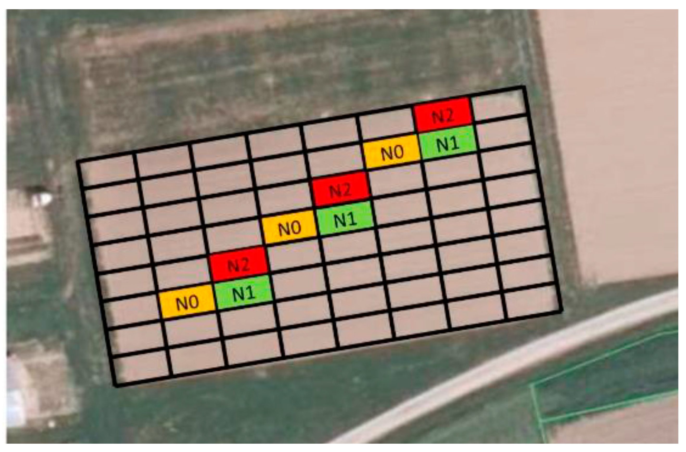
2.1. General Description, Soil, and Physiography of the Dürnast Long-Term Study Area

The Dürnast experimental station is located in Freising (Germany, 30 km north of Munich) in a hilly tertiary landscape, 470 m above sea level. The annual average temperature is 8.4 °C and the average annual precipitation is 823.4 mm. The predominant soil material is tertiary sediment with secondary deposits of Pleistocene loess. The geological situation of the area consists of Pleistocene loess deposition and subsequent erosion in the periglacial period, as well as Holocene erosion and deposition. According to the [38], fine-bodied Dystric Eutrochrept and fine loamy typical Udifluvent are the predominant soil types.

The primary characteristics of the relief and soil parameters are listed in

Table 2. Site description of the long-term nitrogen fertilization experiment in Dürnast [39].

Parameter		Value (Range)
Elevation (m)		470 (469–472)
Slope (rad)		0.05 (0.05–0.09)
Aspect (rad)		2.64 (1.97–3.46)
Soil vertical layer		0–25 cm	25–50 cm	50–75 cm
Soil texture (kg kg−1)	Clay	20.8 (15.7–27.3)	23.3 (15.2–34.9)	26.2 (13.6–34.8)
	Silt	61.5 (54.4–67.5)	61.7 (35.7–72.9)	60.7 (32.8–76.8)
	Sand	16.6 (11.9–21.3)	14.4 (8.5–40.5)	12.4 (5.3–46.8)
	Skeleton	1.2 (0.0–3.0)	0.6 (0.0–7.0)	0.4 (0.0–3.0)
pH		6.44 (5.94–6.84)	6.36 (5.96–7.12)	6.31 (5.98–7.18)
C content (%)		1.18 (0.94–1.38)	0.56 (0.35–1.14)	0.4 (0.22–1.11)
N content (%)		0.1 (0.08–0.12)	0.06 (0.03–0.12)	0.04 (0.02–0.12)

. The area has a slight slope in the south direction with a silt content of approximately 60%. Clay, C, and N increase from the south to the northwest of the area. The relatively high content of C and N in soil layers deeper than 25 cm is evidence of the erosive processes that formed this area.

2.2. General Description Experimental Design, Wheat Varieties, and Amount of Fertilizer

On a 0.23 ha area, a long-term field experiment was established and supervised by the Chair of Plant Nutrition, Freising. Since 1979, potatoes (maize), wheat, and barley have been cultivated in a three-year crop rotation fertilized with six different N fertilizers: calcium ammonium nitrate (KAS), urea (Ha), ammonium sulfate nitrate (ASA), ammonium nitrate solution (AHL), ammonium sulfate nitrate with nitrification inhibitor (Ntec), and calcium cyanamide (Pka). Two nitrogen levels were examined with a total of four replications. For comparison, two control plots were planted in each replication.

This experiment was conducted in an area that is one of the more fertile areas within Germany. After the German soil evaluation system [40] the soil numbers and tillage numbers range between 67 and 73 and 59 and 69, respectively, and the yields of winter wheat range from 70 to 90 dt ha⁻¹ at an adequate fertilization level. This soil and tillage numbers indicate the level of the site-specific soil fertility. The number is derived mainly from the parameters geology, texture and soil condition (dry, wet, acid, calcareous) and the number 100 shows the most fertile site within Germany.

In this work, only the yields of winter wheat fertilized with calcium ammonium nitrate and the associated control plots were evaluated. Calcium ammonium nitrate fertilizer was selected because this is the most frequently used N fertilizer in Germany. Cultivars and amount of fertilizer are described in

Table 3. Wheat cultivars and the amounts of nitrogen fertilizer.

Year	Wheat Cultivar	N Fertilizer (kg ha−1)
		Low	High
1980	Winter Caribo	100	150
1983	Winter Caribo	100	150
1986	Winter Kronjuwel	100	150
1989	Winter Obelisk	100	150
1992	Winter Orestis	100	150
1995	Winter Astron	100	150
1998	Winter Astron	100	150
1992	Winter Obelisk	100	150
1995	Winter Astron	100	150
1998	Winter Astron	100	150
2001	Winter Ludwig	100	150
2004	Winter Tommi	140	180
2007	Winter Tommi	140	180
2010	Winter Tommi	140	180
2012	Spring Kadrilj	120	180
2015	Spring Lennox	120	180

. This fertilizer was applied at three levels of nitrogen fertilization, which included control plots (N0: control plots with zero N, N1: reduced N fertilized plots, and N2: high N fertilized plots). The seed rate was 350 kernels per m².

The yields of wheat were determined per plot with a combine harvester.

From 1979 until 2016, wheat was 16 times cultivated, including twice with spring wheat in 2012 and 2015. The yields were evaluated without spring wheat and excluding the yield from 1980. The yields of spring wheat were always significantly lower in comparison with winter wheat and the yields from 1980 were still affected by the uniform fertilization during years prior to the experiment as indicated by the yields from the control plots (Figure 1).

Per the Descriptive List of Varieties 1989 [41] (Bundessortenamt), the seven cultivars cultivated between 1983 and 2010 demonstrated similar growth and yield properties. The B wheat cultivar Caribo was registered in 1968, has a medium yield, and has a medium tendency for winter kill. The dates of flowering and maturation are in the middle range compared with the other varieties. In comparison to Caribo, the cultivar Kronjuwel (registered 1980) has a higher yield with otherwise the same properties. The Obelisk (registered 1987) and Orestis (registered 1988) cultivars are winter hardier and again have a higher yield than the previously mentioned cultivar. For Astron, which was registered in 1989, flowering and maturity begin a little later than the previously cultivated varieties, but produces a good yield. Ludwig (registered 1998) has worse properties (less winter hardy, later flowering and maturity) than the previous cultivars. Tommy (registered 2002) is a medium–early cultivar that tends to be less winter hardy, but still has a good yield.

Until 2001, the amount of fertilizer applied was 100 kg N ha⁻¹ on the reduced fertilized plots and 150 kg N ha⁻¹ on the higher fertilized plots. Later, the fertilization level increased to 140 and 180 kg N ha⁻¹, respectively.

2.3. Independent Parameters for the Derivation of Yield

The weather data used were obtained from the weather station of the German Weather Service in Dürnast. This is located about 300 m from the investigation area. In this study, we modelled the weather influence on crop yields using monthly and yearly meteorological parameters and additional indices. Beside the mean temperature and amount of precipitation (yearly, monthly), the indices listed in

Table 4. Overview of the climate variables used in this study.

Variable	Definition/Time Range	Formula for the Derivation of the Indices
Precipitation intensity (PI)	Sum of days on which a certain amount of precipitation occurs
	PI1: >0–1 mm per day	$\mathrm{PI}1={\displaystyle {\displaystyle \sum }_{\mathrm{i}=1}^{\mathrm{n}}}\mathrm{P}>0 \mathrm{mm}+\mathrm{P}\le 1 \mathrm{mm}$
	PI2: >1–10 mm per day	$\mathrm{PI}2={\displaystyle {\displaystyle \sum }_{\mathrm{i}=1}^{\mathrm{n}}}\mathrm{P}>1 \mathrm{mm}+\mathrm{P}<10 \mathrm{mm}$
	PI3: >10 mm per day	$\mathrm{PI}3={\displaystyle {\displaystyle \sum }_{\mathrm{i}=1}^{\mathrm{n}}}\mathrm{P}>10 \mathrm{mm}+\mathrm{P}\ge 10 \mathrm{mm}$
	Monthly values from October to August	where P is precipitation (mm) and n denotes number of days
Rain-free days (P0)	Sum of days without precipitation (P0); monthly values from October to August	$\mathrm{P}0={{\displaystyle \sum }}_{\mathrm{i}=1}^{\mathrm{n}}\mathrm{N}=0 \mathrm{mm}$ where N is height of precipitation
Temperature threshold (TT)	Sum of the days on which the threshold values of 5 or 10 °C are exceeded; monthly values from October to August	$\mathrm{TT}1={{\displaystyle \sum }}_{\mathrm{i}=1}^{\mathrm{n}}\mathrm{Tmax}\ge 5 °\mathrm{C}$ $\mathrm{TT}2={{\displaystyle \sum }}_{\mathrm{i}=1}^{\mathrm{n}}\mathrm{Tmax}\ge 10 °\mathrm{C}$ where Tmax is the daily maximum temperature (°C)
Summer days (SD)	Sum of the days on which the air temperature exceeds 25 °C; monthly values from October to August	$\mathrm{SD}={\displaystyle {\displaystyle \sum }_{\mathrm{i}=1}^{\mathrm{n}}}\mathrm{Tmax}\ge 25 °\mathrm{C}$
Heat days (HD)	Sum of the days on which the air temperature exceeds 30 °C; monthly values from October to August	$\mathrm{HD}={\displaystyle {\displaystyle \sum }_{\mathrm{i}=1}^{\mathrm{n}}}\mathrm{Tmax}\ge 30 °\mathrm{C}$
Frost days (FT)	Sum of the days on which the air temperature falls below the value 0 °C; monthly values from October to August	$\mathrm{FT}={{\displaystyle \sum }}_{\mathrm{i}=1}^{\mathrm{n}}\mathrm{Tmin}\ge 0 °\mathrm{C}$ where Tmin is the daily minimum temperature (°C)
Average temperature (Ty) per year		${\mathrm{T}}_{\mathrm{y}}=\frac{\left({{\displaystyle \sum }}_{\mathrm{i}=1}^{\mathrm{n}}{\mathrm{Temp}}_{\mathrm{d}}\right)}{\mathrm{n}}$ where Tempd is the diurnal mean air temperature of the day, n is the number of days per year
Average temperature (Tv) main vegetation period		${\mathrm{T}}_{\mathrm{v}}=\frac{\left({{\displaystyle \sum }}_{\mathrm{i}=1}^{\mathrm{n}}{\mathrm{Temp}}_{\mathrm{d}}\right)}{\mathrm{n}}$ where n is the number of days per main vegetation period
Precipitation sum (Py)	Sum of precipitation per year, (calculated for every year)	${\mathrm{P}}_{\mathrm{y}}={{\displaystyle \sum }}_{\mathrm{i}=1}^{\mathrm{n}}{\mathrm{P}}_{\mathrm{d}} \mathrm{mm}$ where Pd is precipitation per day
Rain factor (RF)	Relationship of precipitation/temperature per year, (calculated for every year)	$\mathrm{RF}=\frac{{\mathrm{P}}_{\mathrm{y}}}{{\mathrm{T}}_{\mathrm{y}}}$ where Py is the annual precipitation and Ty is the average annual temperature
Dryness index de Martonne-Reichel (DI)	Evaluates the effect of precipitation on plant physiology and precipitation distribution during the main vegetation period	$\mathrm{DI}=\frac{{\mathrm{P}}_{\mathrm{y}}}{{\mathrm{T}}_{\mathrm{y}}+10}\times \frac{\mathrm{K}}{120}$ where 10 indicates that negative values in the denominator should be avoided, K is the number of days with precipitation ≥ 1.0 mm, and 120 is the multiannual average number of days with precipitation in Germany (main vegetation period)
Air humidity (AH)	Evaluates the effect of precipitation on plant physiology; annual values	$\mathrm{AH}=\frac{{\mathrm{P}}_{\mathrm{y}}}{{\mathrm{T}}_{\mathrm{y}}+10}$
Aridity index (AI)	Evaluates the effect of precipitation on plant physiology; main vegetation period	$\mathrm{AI}=\frac{{\mathrm{P}}_{\mathrm{v}}}{{\mathrm{T}}_{\mathrm{v}}+10}$
Summer index (SIy)	Sum of days with daily maximum of air temperature above 5 °C; yearly	${\mathrm{SI}}_{\mathrm{y}}={\displaystyle {\displaystyle \sum }_{\mathrm{i}=1}^{\mathrm{n}}}\mathrm{Tmax}\ge 5 °\mathrm{C}$
Summer index (SIv)	Sum of days with daily maximum of air temperature above 5 °C; main vegetation period	${\mathrm{SI}}_{\mathrm{v}}={\displaystyle {\displaystyle \sum }_{\mathrm{i}=1}^{\mathrm{n}}}\mathrm{Tmax}\ge 5 °\mathrm{C}$
Winter index (WI)	Sum of days with daily maximum of air temperature above 5 °C from November to April	$\mathrm{WI}={\displaystyle {\displaystyle \sum }_{\mathrm{i}=1}^{\mathrm{n}}}\mathrm{Tmax} \ge 5 °\mathrm{C}$
Frost alternating days (FAD)	Sum of days (October to April) with a change of temperatures above and below 0 °C within a day, between consecutive days	$\mathrm{FAD}={\displaystyle {\displaystyle \sum }_{\mathrm{i}=1}^{\mathrm{n}}}\mathrm{Tmax}>0+{\displaystyle {\displaystyle \sum }_{\mathrm{i}=1}^{\mathrm{n}}}\mathrm{Tmin}<0$
Early frost index (EFI)	Sum of the days on which the minimum air temperature falls below 0 °C from July to October	$\mathrm{EFI}={\displaystyle {\displaystyle \sum }_{\mathrm{i}=1}^{\mathrm{n}}}\mathrm{Tmin}<0 °\mathrm{C}$
Late frost index (LFI)	Sum of the days on which the minimum air temperature falls below 0 °C from April to July	$\mathrm{LFI}={\displaystyle {\displaystyle \sum }_{\mathrm{i}=1}^{\mathrm{n}}}\mathrm{Tmin} < 0°\mathrm{C}$
Variable	Definition/Time Range
Frost severity (FS)	Annual minimum of temperature
Begin/end of the main vegetation period	First week of the year on which the threshold value of 5 °C is permanently exceeded (at least 5 days)/mid-August
Frost index per Liu (FI_Liu)	Sum of the days on which the minimum air temperature is below −3 °C and the temperature difference is at least 8 °C from the mean value of the last 20 days; from September to May
Frost shock (FS)	Sum of the days on which the air temperature drops by 15 °C within 24 h and the minimum air temperature falls below −3 °C; annual values
Summer cold per Liu (SC_Liu)	Sum of the difference between the minimum temperature and the mean minimum temperature of the last 20 days exceeding 8 °C
Climatic main vegetation time duration 1 (CL1)	Number of days with the longest period in which the air temperature exceeds 10 °C; values per year
Climatic main vegetation time duration 2 (CL2)	Number of 5-day periods with a maximum diurnal air temperature above 10 °C; values per year
Global radiation (GR)	Sum of global radiation; annual values

Compiled from [23,24,25].

were used as independent variables.

2.4. Statistical Analyses

The statistical analysis was completed using SPSS v 24.0 [42]. To achieve the aims of the experiment and answer the experimental question, two different evaluation methods were used.

2.4.1. Calculation of Dataset 1

A fitting function was first calculated with the autoregressive integrated moving average (ARIMA) procedure for the yields of every fertilization level. It consists of three components: autoregression, difference, and moving average. The autoregression indicates which past values were used to predict the current values. The differentiation is needed if trends exist in the time series that need to be removed. The moving average indicates how much the mean values of the time series for past values deviate from the current forecasts (IBM, 2011).

$$y_t= {\alpha }_1{y}_{t-1}+{\alpha }_2{y}_{t-2}+\cdots +{\alpha }_p{y}_{t-p}+{\epsilon }_t+{\beta }_1{\epsilon }_{t-1} +{\beta }_2{\epsilon }_{t-2}+\cdots +{\beta }_q{\epsilon }_{t-q}$$

(1)

The value y of a time series at time t can therefore be determined from the p past values of the time series itself (y_t−1, y_t−2, y_t−p) and the information from the actual variable. The parameter q ≥ 0 specifies how many past values of the residuals (ε) affect the time series. The terms α and β are additional coefficients

The fitted yields were subtracted from individual observations (Y_observed):

$${\mathrm{Y}}_{\mathrm{residual}}={\mathrm{Y}}_{\mathrm{observed}}-{\mathrm{Y}}_{\mathrm{smoothing} \mathrm{yield} \left(\mathrm{ARIMA}\right)}$$

(2)

Y_residual was then the dependent input data for the regressions.

This procedure was necessary because agricultural yields are determined by a variety of influences that complicate modeling. Different cultivars and varying nutrient supply and diseases have direct or indirect influences on crop yields. If these factors were quantifiable, they could be systematically ruled out as crop yield influences. However, in most cases, this is not possible because many data are not sufficiently documented. This method eliminates the long-term trend of growth without ignoring the particularly large upward or downward fluctuations on an annual basis [19]. According to [43,44], influences on yields can be eliminated using a linear trend adjustment and the factors that remain in the smoothed data. Notably, the weather influences remain implicitly embedded in detrended crop yield values. The influences that can be eliminated by the residual line are shown in

Table 5. Overview of the effects on the temporal yield development and the effects that are eliminated by calculating residuals.

Influence	Effects Eliminated by Residuals	Effects Remain in Residuals
Biological and chemical	New varieties Herbicides Insecticides Fertilizer, fertilization level	Diseases Pest infestation
Mechanical management	Technical Equipment Processing
Management advancement	Crop rotation
Atmospheric	Climate change	Weather deviations, Extreme weather events

Modified from Sterzel (2007).

.

2.4.2. Calculation of Dataset 2

The unchanged measured yield was used as the dependent variable. This evaluation was performed without considering the aforementioned limitations. Here, the modelling partly overlapped with the four groups of influencing factors listed in Table 5.

2.5. Statistical Procedures

For both evaluation methods, stepwise regressions were used. The theoretical model of a regression is

$$y_i=b_o+b_1\times x_1+b_2\times x_2+b_n\times x_n+e_j$$

(3)

where the dependent variable (y_i) indicates the wheat yield for every fertilization level; x_i, …, x_n indicate the climatic variables; b₀, …, b_n are the empirical regression model coefficients; and e_j is the residual error component of the model.

Multiple regression models require that the four primary assumptions be met. These assumptions were tested with the following procedures:

• Autocorrelation of regression residuals: Durbin–Watson test;
  If residuals are not independent, there is autocorrelation. This means that a variable correlates with itself at a different time. We use SPSS to test first-order autocorrelation and thus whether a residual correlates with its direct neighbor. However, in this study, it would make little sense to check autocorrelation because it is very unlikely that the measurements or residuals with a distance of three years are dependent. In such cases, testing the independence of the residuals can be omitted.
• Homoscedasticity (no autocorrelation in regression residuals, homogeneity of variance): plot of residuals against predicted values;
• Normally distributed residuals; and
• Multicollinearity (two independent variables are highly correlated): tolerance and variance inflation factor (VIF).

All regression formulas that did not meet these criteria are indicated in the text.

For the models, the variables used were tested for normal distribution (0.05 significance level, Kolmogorov–Smirnov test with the significance correction according to Lilliefors). Non-normally distributed variables were transformed.

In the last step, the predicted values were tested against the measured values with root-mean-squared difference (RMSD):

$$\mathrm{RMSD}={\left[1/\mathrm{N}{\displaystyle \sum }_{\mathrm{i}=1}^{\mathrm{N}\left(\mathrm{h}\right)}{\left({\mathrm{Z}}_{\mathrm{si}}-{\mathrm{Z}}_{\mathrm{si}}^{*}\right)}^2\right]}^{0.5}$$

(4)

where N represents the number of years, z_si is the observed value, and z*_si is the predicted value.

The RMSD is a measure of the accuracy of the prediction calculation, and this value is small for an unbiased prediction.

3. Results

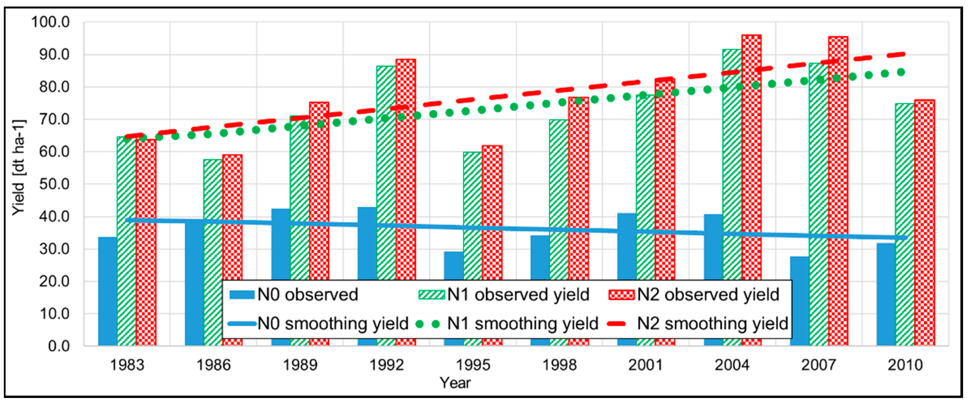
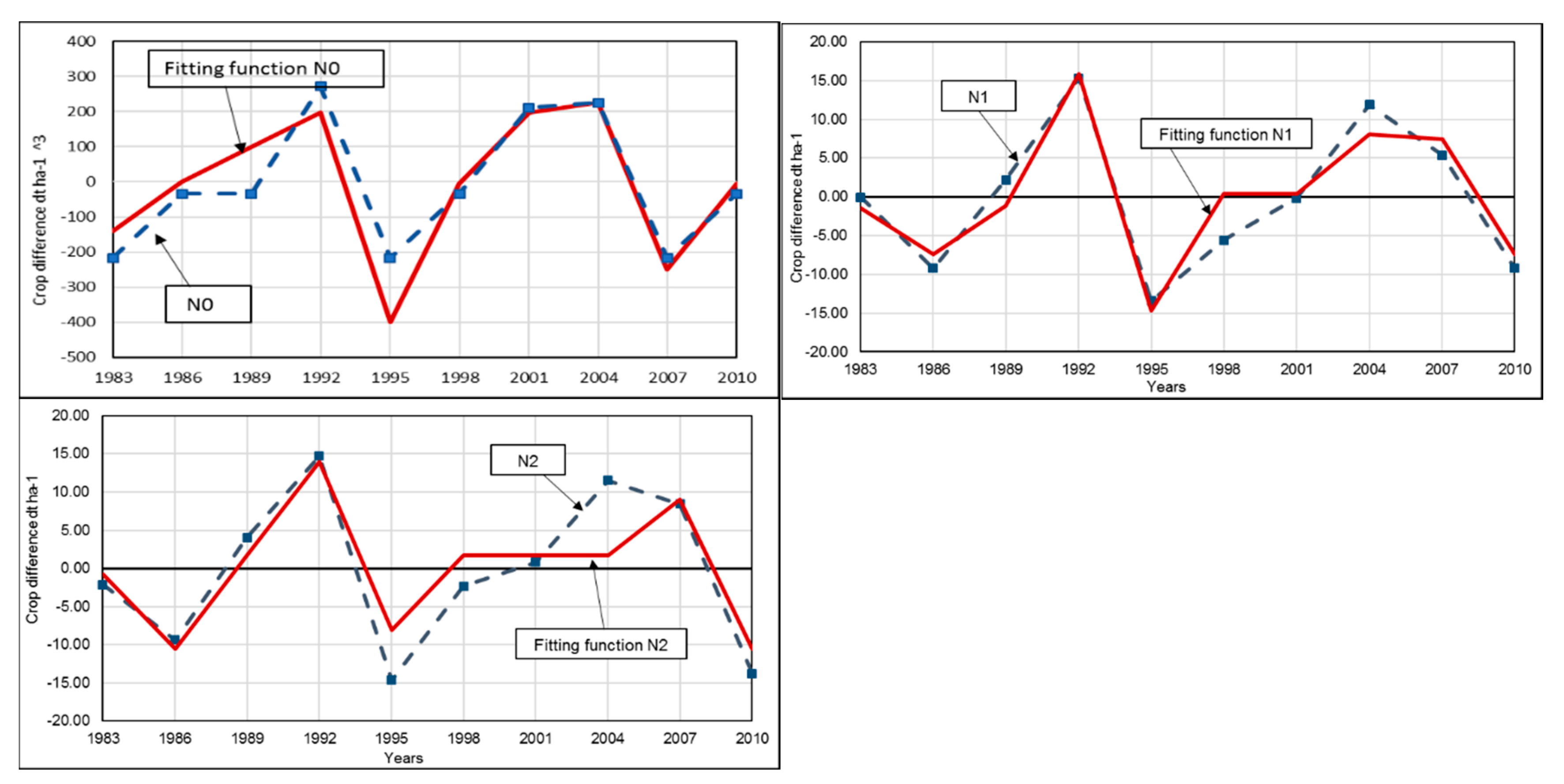
3.1. Temporal Course of the Yields

From 1983 to 2010, the fertilized treatments produced yield values of about 74 and 77 dt ha⁻¹ for the low and high fertilized experimental plots with a range of 57 to 91 and 59 to 96 dt ha⁻¹, respectively. The higher level of N fertilization produced less than 5% higher yields in comparison to the low fertilized plots, which however was statistically not significant. The mean yield of non-fertilized plots was 35.2 dt ha⁻¹, which was approximately half of the yield of the fertilized treatments.

The smoothing lines in Figure 2 indicate an opposite trend between the fertilized variants and the control plots. For the latter, yields reduced by an average of approximately 6%. For the fertilized variants, yields increased by approximately 25% (23% low fertilized, 28% high fertilized).

Progress in breeding and thus biological, chemical, mechanical, and management advancement was also applied to the control plots, but the lack of fertilization was the main factor influencing yield.

3.2. Derivation of Yields with Monthly Predictors

Table 6. Formulas depicting multiple linear regressions derivation of residuals and yields for different levels of fertilization with monthly climate parameters.

	Regression Coefficient	Unit Predictor	Sig.	β Coefficient Standardized	RMSE (dt ha−1)	R2 Adj.
Residuals unfertilized control^3	271.42		**		4.27	0.775
	−61.007 × temperature threshold 2 (TT2) April	number of days	**	−0.822
	319.656 × TT2 February	number of days	*	0.492
Residuals low fertilization level	−22,035		*		2.90	0.862
	1.859 × N0 June	number of days	**	0.651
	−1.532 × temperature threshold 1 (TT1) December	number of days	**	−0.446
Residuals high fertilization level	−46.209		***		4.04	0.804
	2.835 × rain-free days (P0) June	number of days	***	0.909
Yield unfertilized control	43.902		**		3.60	0.487
	−1.499 × temperature threshold 2 (TT2) April	number of days	*	−0.738
Yield low fertilization level	90.973		**		7.63	0.471
	−3.142 × temperature threshold 1 (TT1) December	number of days	*	−0.728
Yield high fertilization level	29.120		n.s.		8.65	0.472
	2.968 × rain-free days (P0) June	number of days	*	0.729

Note: N0, N1, and N2 indicate fertilization control, and low and high fertilized treatments, respectively; *, ** and *** indicate 5%, 1% and 0.01 levels of significance, respectively; n.s., not significant.

indicates the results of the regressions with monthly independent variables, divided into derivations of the yields, expressed as residuals and as unchanged values. We found that temperature and precipitation were significant predictors in all variants, but not as mean values or sums, but in the form of special indices (Table 6). The unit of the indices were exclusive to the temporal duration of a climate situation. The dominating predictors were temperature threshold (TT) and rain-free days (P0), but both had an opposing importance between the calculations. The standardized β coefficient indicates the importance of these indices. The TT decreased from the unfertilized derivation to the high fertilized variant. In contrast, the importance of the number of days without precipitation increased with higher fertilization. The same was found for the calculations of the yields. Whereas the regressions of the residuals had an adjusted determination coefficient (R²) higher than 0.77, the derivation quality of the yields was distinctly weaker. In the latter, the same plant cultivar combined with the same treatment produced different yield-influencing effects. Soil differences between plots were also conceivable.

The gradation described above is also reflected in the calculations of the root mean squared error (RMSE): With increasing yields, RMSE values increased. Deviations until about 2.8−4.3 dt ha⁻¹, in combination with an R² of higher than 0.77, indicated sufficient accuracy.

The quality of the derivations is indicated in Figure 3 and Figure 4. Whereas the fitting line of the residuals on the N0 plot follows the observed values, we found differences in the N1 treatment and particularly for the N2 treatment. In both cases, the worst derivation occurred in 2004, which may be due to the higher yields in this year. Of all investigated years, 2004 showed the highest yields of the fertilized cultivars. The real cause of this finding remains unclear. The divergence between observation and regression of the yields (N2) was distinctly lager, especially in 1995 and 2004 in all treatments.

3.3. Derivation of Yields with Annual Predictors

The application of annual climate variables (

Table 7. Formulas depicting multiple linear regressions derivation of residuals and yields for different levels of fertilization with yearly climate parameters.

	Regression Coefficient	Unit Predictor	Sig.	β Coefficient, Standardized	RMSE (dt ha−1)	R2 Adj.
Residuals unfertilized control	19.697		**		4.41	0.403
	−1.056 × aridity index (AI)	number of days	**	−6.85
Residuals low fertilization	−5.752		n.s.		6.35	0.439
	3.595 × early frost index (EFI)	number of days	*	0.708
Residuals high fertilization	−11.914		*		5.03	0.648
	3.526 × early frost index (EFI)	number of days	*	0.636
	1.960 × winter index (WI)	number of days	*	0.486
Crop unfertilized control	58.083		**		3.73	0.45
	−1.171 × aridity index (AI)	number of days	*	−0.715
Crop low fertilization	72.608		**		5.07	0.733
	−1.830 × summer cold per Liu (SC_Liu)	number of days	**	−0.686
	3.990 × early frost index (EFI)	number of days	**	0.625
Crop high fertilization	−173.24		*		5.90	0.719
	−0.00021 × global radiation (GR)	watt-hour m2	**	0.692
	4.194 × early frost index (EFI)	number of days	*	0.579

Note: N0, N1, and N2 indicate control, and low and high fertilization levels, respectively; *, ** and *** indicate 5%, 1% and 0.01 levels of significance, respectively; n.s., not significant.

, Figure 4) as predictors did not provide as clear a picture as the monthly values and were less accurate, as indicated by higher R² and lower RMSE (Table 6). The R² of the unfertilized plots was weak with the single predictor aridity index (AI). The derivation of the residuals of the fertilized plots with the independent variables early frost index (EFI) and winter index (WI) had a lower R². The accuracy of the regression improved the more predictors were included. However, the quality of the yearly predictors was poor. In all cases, the temporal duration was expressed as number of days.

The application of the observed yields when independent variables—early frost index (SC_Liu) and global radiation (GR)—beside early frost index (EFI) were included, formed a more complex picture. Yield from high fertilization was highly influenced by global radiation.

In most regressions, we noted the frequent occurrence of indices that demonstrate the influence of winter (EFI, WI, TT) and summer (SC_Liu) coldness. The index days without precipitation (P0 in June) also occurred frequently. More common indices, like global radiation (GR) and aridity index (AI), were only detectable when using annual values as predictors.

4. Discussion

The occurrence of winter indicators was noticeable in the monthly and annual values, especially on the unfertilized variants and, to a lesser extent, in the calculations of fertilized yields. One reason for this is the soil conditions. The available field capacity of this site is around 241 mm up to 100 cm of soil depth (according to [38]), this is classified as high) and 325 mm up to 140 cm soil depth. At the beginning of the main vegetation season in March/April, the maximum amount of available field water capacity is reached, so a wheat stand can grow almost completely without irrigation. The soil water content is also temporarily improved by the addition of slope water. The precipitation therefore does not play a direct role in the calculation. In the low and high fertilization levels, however, the climate variable of precipitation-free days in June was significant. The standardized β coefficients showed that the importance of the precipitation-free days in June increased with increasing fertilization, likely due to the higher biomass yield and the associated increase in water consumption of the crop. A further important factor is the relief in the areas. The experimental field is located in a small valley, which allows cold air to accumulate temporarily. The outflow of cold air is delayed by the downhill forest stand. Overall, the predictors of the monthly values led to adjusted R² values of at least 0.7.

The annual figures (Figure 4) showed a weaker relationship. The adjusted R² values were 0.4 for the unfertilized control and low fertilization, and 0.65 for the highly fertilized plots. Winter values were also significant here (EFI and WI). In the following, the significant climate variables are presented.

In 1985, the first days with frost occurred in October. The wheat was sown at the beginning of October, so the phase of emergence was influenced by frost. In the regression analysis, the early frost index proved to be significant. However, we were unable to determine whether early frost was a restriction in all growing years, as the sowing rate fluctuates between early October and early November. If the emergence of wheat is not finished before the first days of frost, wintering damage may occur as the wheat grain is very sensitive to frost [45] (p. 318). Additionally, the winter index, temperature threshold in December and February also proved to be significant in the regression analysis.

For the transition from the vegetative to the generative phase, temperatures around the 3–4 °C are necessary for a longer period of time. Vernalization removes shooting inhibition and the plants enter the generative phase and begin to grow in length. If this cold stimulation does not occur, the plants remain in the vegetative phase [45]. In the same phase, however, most frost damage occurs at low temperatures as the plants are very sensitive in this phase and the vegetation cone is no longer protected by the leaf sheath close to the soil surface [11]. In 1983 and 1986, which experienced constant frost in February, the wheat was affected by the frost.

Here, the winter hardiness of the plants was found to be responsible for the yield losses. The extent to which a plant is damaged by frost depends on the temperatures, the duration of frost events, the insulating effect of a layer of snow, the stage of development, and the variety [10].

Infection with pathogens of individual wheat diseases usually occurs in the months of May and June in appropriate weather conditions. In 1983, 1995, 1998, 2007, and 2010, infections with Puccinia striiformis, Blumeria graminis f. sp. tritici, Septoria tritici, and Fusarium graminearum were possible due to the wetness. Late sowing of winter wheat is a strategy to prevent the occurrence of these diseases. Other strategies include the avoidance of excess nitrogen, the cultivation of resistant or tolerant varieties, clean soil treatment to combat volunteer grain, and fungicide treatment. [46] investigated yield losses of winter wheat from 2003 to 2008 in trials of 12 German federal states. Here, the highest yield losses were caused by Septoria leaf blotch (Mycosphaerella graminicola) with yield reductions of about 7 dt ha⁻¹. Brown rust (Puccinia triticina) also occurred in all German federal states and were second most important in both occurrence and yield loss [47]. No surveys of this kind were conducted on the trial site investigated here. However, losses cannot be ruled out.

A drought in June also negatively influenced the yield. In the regression analysis, the rain-free days in June proved to be significant. Based on long-term records, during this period wheat is in the phase of flowering or grain filling. The optimum temperature for these development stages is 21 °C [37]. To avoid heat stress, different plant responses are known (shortened life cycle, a higher rate of phenological development, and a more efficient use of reserves [14,35]). However, a shortened life cycle means that the thousand-grain weight is reduced, since fewer assimilates can be stored in the grain, which leads to a reduction in yield.

The plant can also try to minimize water loss and maximize water uptake through improved root growth or premature senescence of older leaves [12,14]. Due to the premature senescence of the older leaves, not all assimilates can be stored in the grain, which leads to a lower thousand grain weight and thus to a lower yield.

Whether the plant has really been affected by the drought is difficult to judge. As already mentioned, the soil at the experimental station has a high usable field capacity due to the high silt and soil carbon content. If the soil water supply is well-filled during the winter months, the plant can also produce good yields with less rainfall. However, no conclusion can be drawn about the soil water supply in June, as the necessary information was not considered. Excessive precipitation during this period can also negatively impact yield. If the precipitation is too high, the water can no longer flow off unhindered, so it accumulates. This waterlogging causes abiotic stress in the plants. Stagnant moisture can lead to premature ripening of the wheat in the phases of grain shifting (initiation of individual flowers) and flowering, which results in a shortened grain filling phase and thus to a yield reduction due to lower thousand grain weights [9].

Due to the high silt content, the soil at the experimental station also tends to silt. Due to the silting, the rainwater can no longer infiltrate and flows off. Erosion occurs [48].

In summary, the modelling showed a balanced relationship between complexity and robustness, which minimizes both structural- and parameter-related errors. If the concept of location is assumed, these calculations can also be improved. In addition to weather conditions, relief and soil can be included.

In addition to the chosen statistical method, there is also the possibility of using artificial intelligence methods. Here, possible non-linearities contained in the relationships between climate and yields can also be taken into account.

Earlier studies showed that wheat yields can be well represented by topographic parameters and soil conductivity. However, the annual range was variable (unfertilized: R² of 0.76–0.95, in 1980, 1983, 1989, 1995, 1998, 2001, 2004, 2007, and 2012 and R² of 0.46–0.66 in 1986, 1992, and 2010) [39].

For farming, the results can be used to make appropriate management decisions about seeding, fertilization, and irrigation [49]. During the actual growing season, climate data are available the day prior. The knowledge of the growing stage, the current climate, and the results of the regressions above provide the opportunity to react, for example, with the fertilization. For example, if temperature threshold days during late emergence or in April are met, N fertilization should be reduced.

5. Conclusions

The aim of this work was to determine the influence of climate parameters on the wheat yield grown in one of the more fertile areas in Germany. Not all aspects of climate that account for yield differences can be assayed with monthly or annual indices as used in this study. In this study, the short-term influencing factors were derived by subtraction of the smoothing yield development from the measured yield. The remaining residuals indicated the short-term inter-annual variation, which were determined by the meteorological factors.

However, these approaches provide an extended comprehensive analysis of dedicated yield assessments as done on this site. For the monthly values, the rain-free days in June and the temperature thresholds in April, February, and December were significant. For the annual values, the climate humidity, the early frost index, and the winter index were significant.

The use of such climate parameters in the calculations differed from other analyses where only directly measured parameters were used, like temperature, precipitation, and global radiation [43,44,50].

The results indicate a changed picture of the yield development of this fertile location. The findings that frost and temperature fluctuations are relevant to yields, especially in the transition period from winter to warmer seasons and vice versa, had not been previously described.

A further interesting observation could be made on this site. Different levels of nitrogen fertilization modified the sensitivity to drought and temperature in the case of monthly calculations. The contrary effect of temperature threshold and days without precipitation indicated that higher fertilized crops reacted more sensitively to the impact of drought and less to the temperature threshold. This finding is remarkable, since the difference in yield between high and low fertilized, was only 2–3 dt ha⁻¹ on a multi-annual average due to a reduction of fertilizing by 20–30%. In other words, 20–30% less fertilization reduced the sensitivity to a lack of precipitation on this site. However, this hypothesis needs further verification.

However limitation of this regression should be further considered. The current calculation is only valid for the respective site with its unique climate situation, soil data and applied farming practice. The climate data represent only by a nearby weather station, which can only provide selective information. However, it may be prudently concluded that the same conclusions probably apply on a regional level.

This regression was not constructed for the testing of the effects of climate change. The listed calculations are black box models, which imitate reactions without knowing the effect of the individual influencing parameters. Here, it is sufficient that the model shows the same behavior as the original. The black box modelling is empirical, meaning it is based on observations of behavior (input and output data). The advantage of this type of modelling is that complex (sometimes even impossible) causal analyses can be inferred and powerful and computer-intensive methods are available for this purpose. The application of such analyses have become increasingly accepted. Accurate climate data are essential for input data. These measurements should be recorded where agricultural production is an economic source of income [49].

References

1. Hatfield, J.L.; Boote, K.J.; Fay, P.; Hahn, L.; Izaurralde, R.C.; Kimball, B.A.; Mader, T.; Morgan, J.; Ort, D.; Polley, W.; et al. Agriculture. In The Effects of Climate Change on Agriculture, Land Resources, water Resources, and Biodiversity in the United States; Backlund, P., Janetos, A., Schimel, D., Eds.; U.S. Climate Change Science Program and the Subcommittee on Global Change Research: Washington, DC, USA, 2008; p. 362. Available online: https://www.fs.fed.us/rm/pubs_other/rmrs_2008_backlund_p003.pdf (accessed on 1 November 2019).
2. Hatfield, J.L.; Prueger, J.H. Agroecology: Implications for plant response to climate change. In Crop Adaptation to Climate Change; Yadav, S.S., Redden, R.J., Hatfield, J.L., Lotze-Campen, H., Hall, A.E., Eds.; Wiley-Blackwell: West Sussex, UK, 2001; pp. 27–43. [Google Scholar]
3. Wittwer, S. Food, Climate, and Carbon Dioxide: The Global Environment and World Food Production; CRC Press: Boca Raton, FL, USA, 1995; 236p, ISBN 0-87371-796-1. [Google Scholar]
4. Brassard, J.P.; Singh, B. Effects of climate change and CO2 increase on potential agricultural production in Southern Québec, Canada. Clim. Res. 2007, 34, 105–117. [Google Scholar] [CrossRef] [Green Version]
5. Trinka, M.; Olesen, J.E.; Kersebaum, K.C.; Rötter, R.P.; Brázdil, R.; Eitzinger, J. Changing regional weather-crop yield relationships across Europe between 1901 and 2012. Clim. Res. 2016, 70, 195–214. [Google Scholar] [CrossRef] [Green Version]
6. Peltonen-Sainio, P.; Jauhiainen, L.; Trnka, M.; Olesen, J.E.; Calanca, P.; Eckersten, H.; Eitzinger, J.; Gobin, A.; Kersebaum, K.C.; Kozyrai, J.; et al. Coincidence of variation in yield and climate in Europe. Agric. Ecosyst. Environ. 2010, 139, 483–489. [Google Scholar] [CrossRef]
7. Kristensen, K.; Schelde, K.; Olesen, J.E. Winter wheat yield response to cli-mate variability in Denmark. J. Agric. Sci. 2011, 149, 33–47. [Google Scholar] [CrossRef]
8. Deutschländer, T.; Dalelane, C. Auswertung Regionaler Klimaprojektionen für Deutschland Hinsichtliche der Änderung des Extremverhaltens von Temperatur, Niederschlag und Windgeschwindigkeit; Abschlussbericht, Offenbach am Main, DWD: Offenbach, Hesse, Germany, 2012. [Google Scholar]
9. Wollmer, A.-C.; Pitmann, K.; Mühling, K.-H. Einfluss von temporärer Überstauung auf Wachstum, Nährstoffkonzentration und Ertrag von Weizen. In Thomas Ebertseder (Hg.): Kongressband 2016 Rostock. Vorträge zum Generalthema: Anforderungen an die Verwertung von Reststoffen in der Landwirtschaft. Darmstadt; VDLUFA-Verlag VDLUFA-Schriftenreihe: Darmstadt, Germany, 2016; Volume 73, pp. 138–142. [Google Scholar]
10. Oberforster, M. Resistenz Gegen Biotischen Stress in der Pflanzenzüchtung. Resistenz Gegen Abiotischen Stress in der Pflanzenzüchtung; 63. Tagung, 19–21 November 2012; Lehr- und Forschungsanstalt für Landwirtschaft Raumberg-Gumpenstein: Raumberg-Gumpenstein, Irdning, Austria, 2012. [Google Scholar]
11. Wu, Y.F.; Zhong, X.L.; Hu, X.; Ren, D.C.; Lv, G.H.; Wei, C.Y.; Song, J.Q. Frost affects grain yield components in winter wheat. N. Z. J. Crop. Hortic. Sci. 2014, 42, 194–204. [Google Scholar] [CrossRef]
12. Barlow, K.M.; Christy, B.P.; O’leary, G.J.; Riffkin, P.A.; Nuttall, J.G. Simulating the impact of extreme heat and frost events on wheat crop production: A review. Field Crop. Res. 2015, 171, 109–119. [Google Scholar] [CrossRef] [Green Version]
13. Lüttger, A.B.; Feike, T. Development of heat and drought related extreme weather events and their effect on winter wheat yields in Germany. Theor. Appl. Clim. 2018, 132, 15–29. [Google Scholar] [CrossRef]
14. Barnabás, B.; Jäger, K.; Fehér, A. The effect of drought and heat stress on re-productive processes in cereals. Plant Cell Environ. 2008, 31, 11–38. [Google Scholar] [CrossRef]
15. Asseng, S.; Forster, I.; Turner, N.C. The impact of temperature variability on wheat yields. Glob. Chang. Biol. 2011, 17, 997–1012. [Google Scholar] [CrossRef]
16. Bayerische Landesanstalt für Landwirtschaft Freising (LfL). Weizenkrankheiten—LfL-Merblatt; Bayerische Landesanstalt für Landwirtschaft: Freising, Germany, 2018. [Google Scholar]
17. Hooker, R.H. The weather and the crops in eastern England, 1885–1921. Q. J. R. Meteorol. Soc. 1922, 48, 115–138. [Google Scholar] [CrossRef]
18. Baumann, H.; Weber, E. Attempt of a statistical analysis of the relation between weather and yield by multiple regression. Notes Ger. Natl. Meteorol. Serv. 1966, 37–41. [Google Scholar]
19. Swanson, E.R.; Nyankori, J. Influence of weather and technology on corn and soy bean yield trends. Agric. Meteorol. 1979, 20, 327–342. [Google Scholar] [CrossRef]
20. Chmielewski, F.-M.; Potts, J.M. The relationship between crop yields from an experiment in southern England and long-term climate variations. Agric. For. Meteorol. 1995, 73, 43–66. [Google Scholar] [CrossRef]
21. Alexandrov, V.A.; Hoogenboom, G. Climate variation and crop production in Georgia, USA, during the twentieth century. Clim. Res. 2001, 17, 33–43. [Google Scholar] [CrossRef] [Green Version]
22. Soja, A.-M.; Soja, G. Dokumentation von Auswirkungen extremer Wetterereignisse auf die Landwirtschaftliche Produktion. In Startprojekt Klimaschutz: StartClim.3b—Erste Analysen Extremer Wetterereignisse und ihrer Auswirkungen in Österreich; ARC Seibersdorf Reserach: Seibersdorf, Austria; 106p, Available online: http://141.244.189.116/fileadmin/user_upload/StartClim2003_reports/StCl03b.pdf (accessed on 8 December 2019).
23. Bernhofer, C.; Hänsl, S.; Schaller, A.; Pluntke, T. Charakterisierung von Meteorologischer Trockenheit; Landesamt, F.U., Landwirtschaft, U.G., Eds.; Sächsisches Landesamt für Umwelt, Landwirtschaft und Geologie Dresden, Schriftenreihe: Schriftenreihe, Germany, 2015. [Google Scholar]
24. Beitz, R. Witterung und Klima. Available online: http://www.forstliche-umweltkontrolle-bb.de/r3_klima.php (accessed on 1 January 2020).
25. Riek, W.; Kallweit, R.; Russ, A. Analyse der Hauptkomponenten des Wärmehaushalts brandenburgischer Wälder auf der Grundlage regionaler Klimaszenarien—Abgrenzung von Risikogebieten und Schlussfolgerung für ein Klima-Monitoring. Wald. Landsch. Nat. 2012, 13, 17–32. [Google Scholar]
26. Dendl, M. Ertragsschwankungen von Weizen und Gerste und deren Ursachen in Ausgewählten Bundesländern Deutschlands. Diploma Thesis, Technische Universität München, Lehrstuhl für Pflanzenernährung, Freising, Germany, 2008; p. 50, submitted. [Google Scholar]
27. Olszynski, A. Der Einfluss von Niederschlag und Temperatur auf die Ertragsentwicklung von Weizen, Gerste und Mais in ausgewählten Landkreisen Bayerns unter besonderer Berücksichtigung der Entwicklungsstadien. Bachelor’s Thesis, Technische Universität München Lehrstuhl für Pflanzenernährung, Freising, Germay, 2013; 85p. submitted. [Google Scholar]
28. Lobell, D.; Field, C. Global scale climate-crop yield relationships and the impacts of recent warming. Environ. Res. Lett. 2007, 2. [Google Scholar] [CrossRef]
29. Lobell, D.B.; Ortiz-Monasterio, J.I.; Anser, P.; Matson, P.A.; Naylor, R.L.; Falcon, W.P. Analysis of wheat yield and climatic trends in Mexico. Field Crop. Res. 2005, 94, 250–256. [Google Scholar]
30. McMaster, G.S.; White, J.W.; Hunt, L.A.; Jamieson, P.D.; Dhillon, S.S.; Ortiz-Monasteriop, J.I. Simulating the Influence of Vernalization, Photoperiod and Optimum Temperature on Wheat Developmental Rates. Ann. Bot. 2008, 102, 561–569. [Google Scholar] [CrossRef]
31. Wheeler, T.R.; Craufurd, P.Q.; Ellis, R.H.; Porter, J.R.; Vara Prasad, P.V. Temperature variability and the yield of annual crops. Agric. Ecosyst. Environ. 2000, 82, 159–167. [Google Scholar]
32. Mäkinen, H.; Kaseva, J.; Trnka, M.; Balek, J.; Kersebaum, K.C.; Nendel, C. Sensitivity of European wheat to extreme weather. Field Crop. Res. 2018, 222, 209–217. [Google Scholar] [CrossRef]
33. Gupta, N.K.; Gupta, S.; Kumar, A. Effect of Water Stress on Physiological Attributes and their Relationship with Growth and Yield of Wheat Cultivars at Different Stages. J. Agron. Crop. Sci. 2001, 186, 55–62. [Google Scholar] [CrossRef]
34. Stone, P.J.; Nicolas, M.E. Wheat cultivars vary widely in their responses of grain yield and quality to short periods of post-anthesis heat stress. Aust. J. Plant Physiol. 1994, 21, 887–900. [Google Scholar] [CrossRef]
35. Wang, X.; Hou, L.; Lu, Y.; Wu, B.; Gong, X.; Liu, M. Metabolic adaptation of wheat grain contributes to a stable filling rate under heat stress. J. Exp. Bot. 2018, 69, 5531–5545. [Google Scholar] [CrossRef] [PubMed] [Green Version]
36. Porter, J.R.; Gawith, M. Temperatures and the growth and development of wheat: A review. Eur. J. Agron. 1999, 10, 23–36. [Google Scholar] [CrossRef]
37. Ghobadi, M.E.; Ghobadi, M.; Zebarjadi, A. Effect of waterlogging at different growth stages on some morphological traits of wheat varieties. Int. J. Biometeorol. 2017, 61, 635–645. [Google Scholar] [CrossRef]
38. Arbeitsgruppe, B. Bodenkundliche Kartieranleitung. 5. Verbesserte und erweiterte Auflage (Herausgegeben von der Bundesanstalt für Geowissenschaften und Rohstoffe in Zusammenarbeit mit den Staatlichen Geologischen Diensten der Bundesrepublik Deutschland; Schweizerbart’sche Verlagsbuchhandlung: Hannover, Germany, 2005. [Google Scholar]
39. Heil, K.; Schmidhalter, U. Improved evaluation of field experiments by ac-counting for inherent soil variability. Eur. J. Agron. 2017, 89, 1–15. [Google Scholar] [CrossRef]
40. Bundesministeriums der Justiz und für Verbraucherschutz. Gesetz zur Schätzung des landwirtschaftlichen Kulturbodens (Bodenschätzungsgesetz—BodSchätzG). Available online: https://www.gesetze-im-internet.de/bodsch_tzg_2008/BodSch%C3%A4tzG.pdf (accessed on 10 October 2019).
41. Bundessortenamt. Beschreibende Sortenliste Getreide, Mais, Ölfrüchte, Leguminosen (großkörnig), Hackfrüchte (außer Kartoffeln). In Bundessortenamt (Beschreibende Sortenliste Getreide, Mais, Ölfrüchte, Leguminosen (großkörnig), Hackfrüchte (außer Kartoffeln)); Bundessortenamt: Hannover, Germany, 2017; ISBN 2190-6130. [Google Scholar]
42. IBM. IBM SPSS Forecasting 20; IBM Corporation: Hannover, Germany, 2011. [Google Scholar]
43. Sterzel, T. Correlation Analysis of Climate Variables and Wheat Yield Data on Various Aggregation Levels in Germany and the EU-15 Using GIS and Statistical Methods, with a Focus on Wave Years; PIK Report PIK-108; Potsdam-Institut fuer Klimafolgenforschung e.V.: Potsdam, Germany, 2007; 122p. [Google Scholar]
44. Gröbmaier, J. Ökonomische Auswirkungen des Klimawandels auf den Marktfruchtbau und Bewertung von Anpassungsoptionen am Beispiel von Ernteversicherung. Ph.D. Thesis, Fakultät Wissenschaftszentrum Freising, Freising, Germany, 2012. [Google Scholar]
45. Lütke Entrup, N.; Schäfer, B.C. Lehrbuch des Pflanzenbaues, 3rd ed.; Agroconcept: Bonn, Germany, 2011. [Google Scholar]
46. Jahn, M.; Wagner, C.; Sellmann, J. Ertragsverluste durch wichtige Pilzkrankheiten in Winterweizen im Zeitraum 2003 bis 2008. Versuchsergebnisse aus 12 deutschen Bundesländern. J. Für Kult. 2012, 64, 273–285. [Google Scholar]
47. Börner, H.; Aumann, J.; Schlüter, K. Pflanzenkrankheiten und Pflanzenschutz, 8th ed.; Springer-Lehrbuch: Berlin/Heidelberg, Germany, 2009. [Google Scholar]
48. Dietz, T.; Weigelt, H. Böden unter landwirtschaftlicher Nutzung: 48 Bodenprofile in Farbe; BLV-Verl.-Ges: München, Germany, 1991; 108p. [Google Scholar]
49. Hoogenboom, G. Contribution of agrometeorology to the simulation of crop production and its applications. Agric. For. Meteorol. 2000, 103, 137–157. [Google Scholar] [CrossRef]
50. White, J.W.; Hoogenboom, G.; Kimball, B.A.; Wall, G.W. Methodologies for simulating impacts of climate change on crop production. Field Crop. Res. 2011, 124, 357–368. [Google Scholar] [CrossRef] [Green Version]
Figure 1. Location of experimental plots (4 × 8 m), fertilized with calcium ammonium nitrate throughout the whole long-term field experiment.
Climate 08 00100 g001
Figure 2. Annual yields of winter wheat between 1983 and 2010 with the smoothing lines for the fertilized and control plots (N0 unfertilized plots, low fertilized plots N1, high fertilized plots N2).
Climate 08 00100 g002
Figure 3. Measured and predicted (see Table 3) residuals with monthly predictors for the different fertilization levels (N0 unfertilized plots, low fertilized plots N1, high fertilized plots N2, N0 expressed as transformed variable).
Climate 08 00100 g003
Figure 4. Measured and predicted (Table 3) residuals with yearly predictors for the different fertilization levels. N0, unfertilized plots; N1, low fertilized plots; N2, high fertilized plots.
Climate 08 00100 g004