Abstract
Water availability in semiarid regions is endangered, which is not only due to changing climate conditions, but also to anthropogenic land use changes. The present study analyzed the annual and monthly water balance (WBc) and the soil moisture deficit (Ds) for different vegetation units under semiarid conditions in the Andes of southern Ecuador, based on limited meteorological station data and field measurements (soil samples). To calculate crop evapotranspiration (ETc) the Blaney–Criddle method was applied, and the specific crop factor (Kc) included, because only temperature (T) and precipitation (P) data were available. By means of the soil samples the water retention capacity (RC) of the different soil types present in the study area were estimated, which, in combination with WBc, provided reliable results respective to water surpluses or deficits for the different vegetation units. The results indicated highest Ds for cultivated areas, particularly for corn and sugarcane plantations, where annual deficits up to −1377.5 mm ha−1 and monthly deficits up to −181.1 mm ha−1 were calculated. Natural vegetation cover (scrubland, forest and paramo), especially at higher elevations, did not show any deficit throughout the year (annual surpluses up to 1279.6 mm ha−1; monthly surpluses up to 280.1 mm ha−1). Hence, it could be concluded that the prevailing climate conditions in semiarid regions cannot provide the necessary water for agricultural practices, for which reason irrigation is required. The necessary water can be supplied by areas coved by natural vegetation, but these areas are endangered due to population growth and the associated land use changes.
1. Introduction
Water and fertile soils are fundamental for agricultural development [1]. However, these resources suffer natural degradation due to erosion processes, floods and droughts as well as from anthropogenic impacts such as deforestation and other land use changes [2,3]. Additionally, population growth and observed climate changes affect water availability in a significant and serious way [4], because higher global mean temperatures result in higher evaporation rates, increased water retention capacity throughout the atmosphere, and changes in atmospheric circulations, which alter the hydrological cycle [5,6]. As the Fifth Assessment Report of the Intergovernmental Panel on Climate Change indicates [7,8], quantity and quality of water will change in many parts of the world, especially in semiarid regions where the water supply is particularly sensitive to precipitation amounts and evaporation rates, which restrict local water availability. Furthermore, soils in these regions generally have low natural productivity and low fertility due to the pronounced precipitation cycle [9], which, in combination with the frequent occurrence of droughts, complicates agricultural development [10,11].
Nonetheless, in semiarid regions, the economic development of the local population depends principally on agriculture, and therefore, on local water availability [12,13], for which reason the observed altered climate conditions and population growth, as well as unsustainable water management practices endanger the availability of this hydrological resource [14]. The agriculture in these regions is generally executed by means of irrigation systems to guarantee food production [15,16], in which water is transported and applied mainly by means of irrigation canals [17], which is why a large amount of water is lost through evaporation, drainage, deep percolation and subsurface runoff, leading to higher production costs and lower plant productivity [2]. In summary, the limited water availability in semiarid regions, together with the predicted changes in climate conditions, combined with unsustainable water management and land use changes (population growth), complicates agricultural development, which is confirmed by the observed decrease in food production (e.g., [18,19]).
For sustainable water management in semiarid regions, the quantities of water for optimal crop productivity must be known, which can be derived from the annual and monthly water balance in combination with the soil moisture content (e.g., [20,21]). These parameters do not only provide information about water availability, but also about the watershed dynamics, including environmental changes (e.g., [4,10]). This information allows for the adoption of strategies for ecosystem protection, as well as for a sustainable use of hydrological resources for agricultural proposes and a continual drinking water supply for the local and regional population (e.g., [16,22]). Nonetheless, the determination of water balance and soil moisture content is still challenging because the stored water quantities and their variation during the year needs adequate climate and specific soil data, which is often unavailable in developing countries (e.g., [23,24]). Furthermore, the variations in soil moisture content, especially in agricultural zones, are difficult to quantify due to uncontrolled water use (irrigation), which also alters land–atmosphere interactions and local hydrological processes (e.g., [25,26,27]).
In Ecuador, semiarid regions are mainly located in the south and along the coast, where concurrently agriculture is the principal economic activity for the population [13,28]. These regions are mostly situated near the transition zone of the northern Peruvian desert, which makes these regions vulnerable to desertification and soil erosion processes, caused by changing climate conditions and anthropogenic activities (land use change) [16,29]. Unfortunately, information about climate and soil characteristics are limited (e.g., [30,31]), which complicates water balance analysis and soil moisture content determination. Nonetheless, these data are necessary to create sustainable water management plans, but to date information about water balance and soil moisture deficits is mostly unavailable.
This also applies to the southernmost province of Ecuador, namely the province of Loja, where the agricultural sector depends on variable climate conditions and local water availability. Therefore, irrigation systems are widely implemented to guarantee crop productivity (e.g., [32,33]). As the National Water Ministry of Ecuador (Secretaría Nacional del Agua, SENAGUA) [33] confirms, existent irrigation systems in this region are mostly irrigation canals, which are poorly managed, for which reason enhanced water consumption, and consequently, a reduction in water availability is observed [34,35]. The inadequate use of irrigation water produces not only a limitation of this resource, but also an alteration in the water–air ratio within the soils, generating low yields and higher production costs, besides the acceleration of salinization processes [36,37].
To offer a solution, the present study calculates water balance and soil moisture deficits during the year for the communities of Malacatos and Vilcabamba, located in the Andes of southern Ecuador, using limited long-term meteorological station data (10 years) in combination with field measurements (soil samples). From these data the retention capacity (RC) of the different soil types is estimated, the mean annual and monthly water balance of the different vegetation units (WBc) calculated, as well as the monthly soil moisture deficit (Ds) determined. The findings should support governmental decision makers and promote the implementation of sustainable water management projects to guarantee water availability and food production for local and regional populations.
2. Study Area and Data
2.1. Study Area
The communities of Malacatos and Vilcabamba are located in the southern Ecuadorian Andes (Province of Loja) between the coordinates UTM 17S 685000–710000 and 9518000–9545500. The communities form part of the headwaters of the Catamayo–Chira catchment, which drains into the Pacific Ocean in northern Peru. This region is characterized by a complex topography, due to ongoing orogenic processes, which created abrupt changes between valleys and ridges [38,39]. The geology in the study area is characterized by sedimentary deposits in the valleys, and metamorphic rocks (Chiguinda Unit) and conglomerates (Cerro Mandango) at the ridges [40]. The elevation ranges between 1100 m asl at the valley bottom and 3800 m asl at the highest mountain tops (Figure 1).
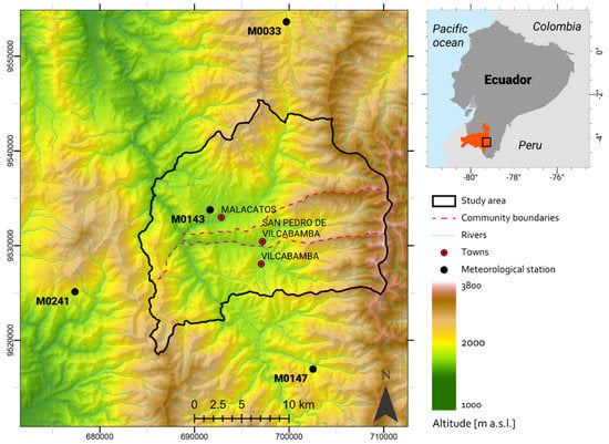
Figure 1.
Digital elevation model (DEM) and limits of the communities Malacatos and Vilcabamba, including the meteorological station locations.
The climate in the study area is semiarid (Figure 2), with a mean annual precipitation of 808.3 mm [31]. The precipitation shows a clear annual cycle with one main rainy season from October to April (austral summer), when over 88% of the total annual rainfall amounts are recorded, and a dry season from May to September (austral winter; [30,39]). The mean annual temperature at lower elevations is 20.1 °C, decreasing with height [16,41].
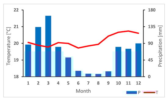
Figure 2.
Climograph of the station Malacatos (M0143), province Loja - Ecuador (period: 2006–2015).
The economy of the local population is principally based on agriculture, in which low-yield products for subsistence dominate [24]. However, in some parts, irrigation systems and intensive agricultural production techniques are implemented to produce principally corn and sugarcane, but also coffee and fruits for the local and regional market [42].
2.2. Data and Materials
Daily precipitation (P) and temperature (T) data for the period 2006–2015 were obtained from the Ecuadorian weather service (Instituto Nacional de Meteorología e Hidrología, INAMHI), which operates four meteorological stations in or next to the study area (see Figure 1; M0033: 4°2′11″ S, 79°12′4″ W; M0143: 4°12′58″ S, 79°16′24″ W; M0241: 4°17′40.6″ S,79°24′6.1″ W; M0147: 4°22′4.5″ S, 79°10′30.2″ W). The digital elevation model (DEM, Figure 1) with a spatial resolution of 30 m was obtained from ASTER (Advanced Spaceborne Thermal Emission and Reflection Radiometer) satellite images from 2011, which can be downloaded from the USGS’s Earth Explorer platform (https://earthexplorer.usgs.gov/). The DEM was re-sampled to a resolution of 100 m [30], due to limited meteorological information and to provide water balance and soil moisture deficit values per hectare (ha). The upscaling was done by means of the software ArcGIS 10.4, which was also used to interpolate the meteorological station data.
The vegetation cover map of the study area in a 1:25000 scale was obtained from the Ecuadorian Ministry of the Environment (Ministerio del Ambiente, MAE), which was generated by means of a supervised classification from orthophotos [43]. The original vector map was converted into a raster format with a resolution of 100 m, which afterwards was reclassified into 11 main categories (Figure 3), particularly corn, sugarcane, coffee, fruits, pastures, scrubland, forest, paramo, eroded areas, urban areas and water surface using the software ArcGIS 10.4.
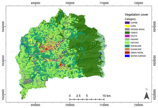
Figure 3.
Vegetation map of the communities Malacatos and Vilcabamba (reclassified; based on [43]).
The remaining natural vegetation in the study area is scrubland at mid and lower elevations, tropical mountain forest at higher elevations and paramo at the upper eastern ridge. The mountain forest ecosystem is characterized by extraordinarily high biodiversity, and, together with the paramo area, provides important services for the local population (e.g., water supply; [44,45,46]. However, the natural ecosystems are endangered, due to population growth and the associated land use changes [47,48]. The anthropogenic impact upon the study area is clearly visible, particularly near the valley bottom and inside the side valleys where agriculture dominates, due to the lower slope gradients. Also, pasture is widely spread, especially at the western ridge, but also at mid and lower elevations at the eastern and northern ridges. Furthermore, eroded areas exist, because former farmland produced enhanced erosion processes at steeper slopes, which degraded the soils [16]. Urban areas are present, too, which comprise of small villages, isolated houses and other human structures, besides water surfaces, particularly rivers and creeks, as well as small lagoons in the paramo area at the upper eastern ridge (Figure 3).
The soil map in the study area was provided by SENAGUA [33] and includes seven specific soil types, namely Fluvent, Hemist (Aquept), Orthent, Torrent, Tropept, Tropept + Orthent and Udalf (Figure 4). A detailed taxonomy of these soil types can be found in the world reference base for soil resources [49]. The necessary soil characteristics to determine the water retention capacity (RC), specifically bulk density (BD) and soil texture parameters, were obtained by means of soil samples (Figure 4). Therefore, Kopecky steel rings with a volume of 113.10 cm³ were used (BD), and additionally at each sampling point 2 kg of soil extracted for further granulometric analysis (soil texture). The samples were analyzed in the soil laboratory of the Technical University of Loja (Universidad Técnica Particular de Loja, UTPL).
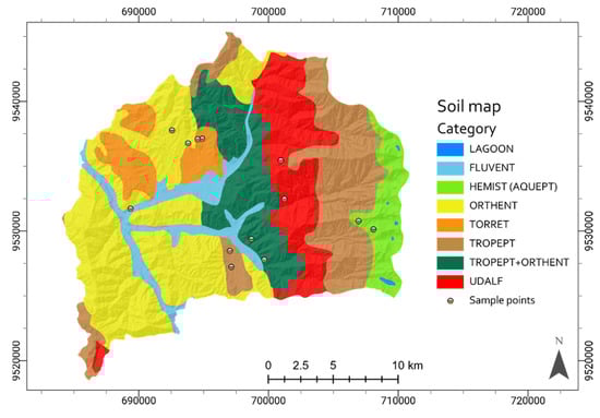
Figure 4.
Soil map of the communities Malacatos and Vilcabamba (adopted from [33]), including sampling points.
3. Methods
3.1. Soil Sampling and Granulometric Analysis
By means of the provided soil map (Figure 4; [33]), two sample points were established for each soil type. At each sample point, a bulk density test was executed to determine the physical properties of the soils [50]. This analysis is especially important for areas of agricultural use and livestock breeding (pasture), because compact soils can reduce productivity and encourage soil erosion processes [47,51,52]. Before executing the test, topsoil was removed and then two Kopecky rings inserted in the subsoil at a depth of 30 cm [28,53]. After sample extraction, the steel rings were immediately covered to avoid moisture loss [54]. Additionally, 2 kg of soil were extracted at each sampling point for further granulometric analysis [55]. All samples were transported in separated closed plastic bags to the soil laboratory of the UTPL, where the soil characteristics were determined.
In the laboratory, first, the weight of the wet soil samples taken by the Kopecky steel rings were determined, which afterwards were oven-dried at a temperature of 110 °C for a period of 24 h. Removed from the oven, the samples were weighed again to obtain their dry weight (Wd). By means of the sample volume (Vs) and its Wd, the bulk density (BD) of the soils was calculated, applying the following equation [56]:
where BD is the bulk density [g/cm³], Wd is the dry weight of the sample [g] and Vs is the volume of the sample [cm³].
To determine the soil texture, the additionally taken 2 kg soil samples were mixed, considering the specific soil type (2 sampling points for each soil type = 4 kg), and afterwards a granulometry analysis executed, applying the hydrometer method [57], which is also established in the Ecuadorian Norm INV E-124. For the hydrometer method, only 50 g of soil is needed, but the mixture of two bigger samples guarantees a representative particle size distribution for each specific soil type [55]. The mixed samples were oven-dried, weighed, and afterwards individually placed in flasks filled with distilled water. Then, a dispersing agent was added, specifically 125 mL of sodium hexametaphosphate, and the samples left to soak overnight to disintegrate the clods. The next day, the samples were transferred to another flask (dispersion glass), distilled water added, and then the assays centrifuged for one minute. After centrifugation, a hydrometer was slowly introduced to avoid disturbing the suspension, as well as a thermometer with a precision of 0.1 °C. Hydrometer and temperature readings were taken after one minute and again after two minutes. Then, both measurement devices were removed and cleaned with distilled water to repeat the procedure an additional two times. All readings were made on the upper part of the meniscus formed around the hydrometer stem. Finally, all readings of a specific soil type were averaged to obtain the percentage of each texture class (sand, loam and clay), which are the necessary input parameters to determine field capacity (FC) and permanent wilting point (PWP) of the different soil types.
3.2. Soil Water Retention Capacity (RC)
The soil water retention capacity (RC) of the soils was determined by means of the texture parameters, particularly the percentage of each particle size fraction, and the calculated BD of each specific soil type. By means of the texture parameters, field capacity (FC) and permanent wilting point (PWP) was calculated, applying the equations proposed by [58] (Equations (2) and (3)). FC is defined as the optimum water level for plants within the soil when all pores are filled with water, whereas PWP is reached when almost all soil moisture is lost due to percolation and evapotranspiration processes, and the remaining water fixed by soil particles unavailable for plants [58]. With this information RC could be calculated for each specific soil type, applying the equation proposed by [59,60] (Equation (4)). Finally, the specific RC values were assigned to each soil type based on the provided soil map (Figure 4), which was also converted into a raster format with a 100 m spatial resolution to obtain values per hectare (ha), using the software ArcGIS 10.4.
where: RC is the soil water retention capacity [mm]; FC is the field capacity [%], PWP is the permanent wilting point [%], BD is the bulk density [g/cm³], DH2O is the water density at 20 °C [0.9982 g/cm³], and Soildepth is depth of the evaluated soil horizon [mm] (here: 300 mm).
3.3. Water Balance (WB)
Mean monthly and annual water balance (WB) for the study area was calculated using the 10-year data set (2006–2015) from the four meteorological stations located in and next to the study area (M0033, M0143, M0241 and M0147, Figure 1). Due to limited station information, only temperature (T) and precipitation (P) data could be included. The WB was calculated for each grid cell (x,y), applying the following equation [61] (Equation (5)):
where: WB(x,y) is the water balance [mm] (positive or negative) at grid cell (x,y), P(x,y) the precipitation [mm] at grid cell (x,y) and ET0(x,y) the reference evapotranspiration [mm] at grid cell (x,y)
In general, if reference evapotranspiration (ET0) is higher than precipitation (P) in a specific month, the month is classified as arid or dry (deficit or negative WB), whereas if precipitation (P) is greater than reference evapotranspiration (ET0) the month is humid or wet (surplus or positive WB) [62]. To calculate WB, first, the monthly and annual P and ET0 maps had to be generated, whose creation is described in the following sections.
3.3.1. Precipitation (P) Maps
To generate the monthly and annual precipitation maps, first, the daily P data of each station was quality checked, controlling for the reliable range of the provided information, which was established by INAMHI Loja (personal comment Ing. Augusto Araque, Regional Coordinator of INMAHI Loja). Negative values and values out of range were eliminated without refill [63], and afterwards, the remaining daily data summed for each individual month, if at least 90% of the daily information was existent (minimum 27 days). Then, the monthly 10-year data set was averaged for each specific month to obtain mean monthly values, which subsequently were used to calculate mean annual values for each station. Finally, the mean monthly and annual P data of all stations were interpolated, applying Ordinary Kriging to generate raster maps in a 100 m resolution for the whole study area [30,39]. This interpolation method was selected because P is highly variable in space and time, and therefore generally no correlations between P and geographic (e.g., latitude) or topographic (e.g., altitude) parameters can be determined [38,64].
3.3.2. Reference Evapotranspiration (ET0) Maps
To calculate reference evapotranspiration (ET0), the SCS modified Blaney–Criddle equation was applied [65,66], because it only needs mean monthly T data as input to predict evapotranspiration reasonably for larger time periods [67]. The ET0 equations can be written as follows [68]:
where: ET0(x,y) is the reference evapotranspiration [mm] at grid cell (x,y), f(x,y) is the percent of total monthly daylight hours at grid cell (x,y), Kt(x,y) is monthly consumptive use coefficient at grid cell (x,y), T(x,y) is the average monthly mean temperature [°C] at grid cell (x,y), and Lp are the hours of daylight during a specific month in relation to the annual hours of daylight [%].
To generate the mean monthly and annual ET0 maps, first, the respective T maps had to be produced. Therefore, the daily T data from each station was quality checked and reliable ranges established [63]. All values out of range were eliminated without refill, and afterwards averaged for each month, if at least 80% of the daily information existed (minimum 24 days). Then, the 10-year data set was averaged for each specific month to obtain mean monthly T values, which subsequently were used to calculate mean annual values.
The lower threshold for T (80%) compared to P (90%) was set, because T does not show high spatiotemporal variability and can be correlated with geographic (e.g., latitude) or topographic (e.g., altitude) parameters [69,70]. Therefore, to interpolate the T data, Kriging with detrended raw data was applied [41], for which, first, specific mean monthly and annual altitudinal gradients for the study area were deviated. The obtained monthly and annual altitudinal gradients were used to “detrend” the station data to a uniform altitude (here: 1000 m asl). Then, the detrended station data were interpolated by Ordinary Kriging to generate an areawide T map at the detrending altitude. Finally, the real vertical distribution of T was re-established for every grid cell (x,y) by means of the calculated mean monthly and annual altitudinal gradients and the DEM (Figure 1). For more information about the detrending technique, please refer to [71].
3.4. Specific Crop Evapotranspiration (ETc) and Water Balance (WBc)
To estimate the evapotranspiration for the different vegetation units (ETc), the specific crop coefficients (Kc) were included in the ET0 calculation (e.g., [72,73]). The specific mean Kc values were taken from [74] for cultivated areas or estimated for natural vegetation units by means of air humidity and evapotranspiration studies realized in tropical forests and at paramo areas in South America [71,75,76,77] (Table 1). The respective Kc values were assigned to every grid cell (x,y) based on the reclassified vegetation map (Figure 2). Finally, the generated monthly ET0 maps were multiplied by the Kc map to obtain the ETc at every grid cell (x,y; Equation (9)).
where: ETc(x,y) is the specific crop evapotranspiration [mm] at grid cell (x,y), ET0(x,y) is the reference evapotranspiration [mm] at grid cell (x,y), and Kc(x,y) is the cultivation coefficient at grid cell (x,y).

Table 1.
Specific crop coefficient (Kc) used for the present study.
By means of the generated monthly Pi and ETci maps the monthly water balance (WBci), specific for each vegetation unit or category, could be calculated, applying the following equation (Equation (10)):
where: WBci(x,y) is the monthly water balance for each vegetation unit [mm] (positive or negative) at grid cell (x,y), Pi(x,y) the monthly precipitation [mm] at grid cell (x,y) and ETci(x,y) the specific monthly crop evapotranspiration [mm] at grid cell (x,y).
3.5. Soil Water Reserve (R) and Soil Moisture Deficit (Ds)
By means of the specific RC for each soil type and monthly WBci maps, the soil water reserve (R) could be estimated. In general, R is the total soil water content available for plants [78], which is refilled during wet months until the RC of a specific soil type is reached. If more water is received, the additional supply is drained superficially or infiltrates to deeper horizons. During dry months, R is reduced by evapotranspiration processes until the wilting point (PWP) is reached, which means that no more water is accessible for plants [79,80].
For this study, monthly R were calculated up to a subsoil depth of 30 cm, because crop roots generally do not reach deeper horizons and evapotranspiration processes are linked to the root system and the upper soil horizons [53,81]. To calculate R for a specific month (i) at grid cell (x,y), R from the previous month (Ri-1) must be considered and added to the actual monthly WBci (Equation (11)). As mentioned before, the limits for R range between RC and PWP (or zero), which leads to two additional conditions (Equations (12) and (13); [82]).
where: Ri(x,y) is the soil water reserve for a specific month [mm] at grid cell (x,y), Ri-1(x,y) is the soil reserve or storage of the previous month [mm] at grid cell (x,y), Pi(x,y) is the monthly precipitation [mm] at grid cell (x,y), ETci(x,y) the monthly specific crop evapotranspiration [mm] at grid cell (x,y), and RC(x,y) is the retention capacity [mm] at the grid cell (x,y).
As [83] indicated, R generally varies between 0 mm and 100 mm, for which reason the monthly R calculations were initiated with the wettest month, assuming a previous monthly reserve (Ri-1) of zero. If water remained in the soil at the end of the year (R > 0), a new monthly R calculation was executed to adjust the initial R value, in which the remaining Ri from the previous calculation was included to close the annual cycle.
To determine the monthly soil water deficit or surplus (Ds) for each grid cell (x,y), first, the monthly reserve variation (VRi; Equation (14)) must be calculated, taking into consideration the actual reserve (Ri) and the reserve of the previous month (Ri-1). By means of the WBci and VRi maps for a specific month (i), the monthly Ds could be calculated for each grid cell (x,y; Equation (15)), which indicates the surplus or deficit of water (mm) for plants to conduct their natural processes. If Ds are negative irrigation is necessary; whereas no additional water is required if Ds are positive [83].
where: VRi(x,y) is the reserve variation for a specific month [mm] at grid cell (x,y), Ri(x,y) is the soil water reserve for a specific month [mm] at grid cell (x,y), and Ri-1(x,y) is the soil reserve or storage of the previous month [mm] at grid cell (x,y).
where: Dsi(x,y) is the monthly soil water deficit or excess [mm] at grid cell (x,y), WBci(x,y) is the monthly water balance [mm] at grid cell (x,y), and VRi(x,y) is the monthly reserve variation [mm] at grid cell (x,y).
4. Results
The hydrometer method determined the percentages of sand, loam and clay of the seven soil types present in the communities of Malacatos and Vilcabamba. Fluvent, Orthent and Hemist soils had a sandy loam texture, Udalf and Tropept a loamy clay texture, Tropept and Orthent a clay texture, and Torret a loamy sandy clay texture. By utilizing this information BD, CC, PWP and RC could be calculated for each specific soil type (Table 2). As mentioned before, RC was calculated for the first 30 cm of subsoil, which is the available soil water for crops (corn and sugarcane), because their roots generally do not reach deeper soil horizons [53].
Table 2.
Soil sample analysis, including mean values for soil texture, bulk density (BD), field capacity (CC), permanent wilting point (PWP) and water recitation capacity (RC).
In general, soil texture determines the RC of a specific soil type, in which sandy soils store less water than clay soils, because the pores between the soil particles are larger, which increase infiltration capacities but reduces RC [84]. Therefore, the highest RC was calculated for clay soils, particularly for Tropept + Orthents (55.09 mm) and Tropept (47.94 mm), which are located at mid and higher elevations in the study area (Figure 4), whereas the lowest RC was obtained for sandy soils, namely Orthents (26.87 mm) and Fluvents (32.65 mm), which are located near the river courses or at flooded land (sedimentation). The clay content of all soil types in the study area was moderate to high (16–77%; Table 2), which makes the soils partially expansive, plastic and impermeable [24]. Nonetheless, the soils are mostly appropriate for agricultural practices, because this requires a clay content between 10% and 30% [85]. A higher clay content leads to reduced infiltration and increased surface runoff during a precipitation event [47,51], which is why less water is available for plants.
Annual and monthly water balance for the specific land covers (WBc and WBci) were calculated by means of the available meteorological station data (P and T). The generated T maps were the basis for the determination of ET0, applying the modified SCS equation [65,72]. Then, the specific crop coefficient (Kc) was integrated to obtain ETc, established by [86]. The mean annual distribution and amounts of P, ETc and WBc for the study area are shown in Figure 5.
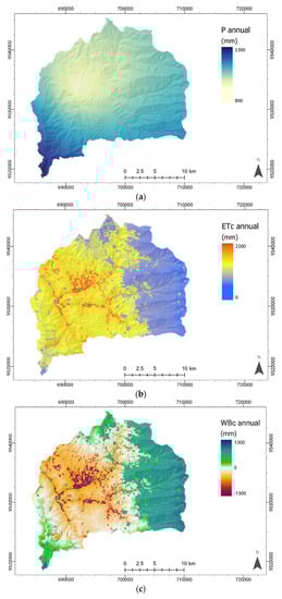
Figure 5.
(a) Annual precipitation (P) of the communities Malacatos and Vilcabamba. (b) Annual crop evapotranspiration (ETc) of the communities Malacatos and Vilcabamba. (c) Annual specific crop water balance (WBc) of the communities Malacatos and Vilcabamba.
Figure 5a illustrates that highest P amounts are observed at the ridges to the east and the west of the communities of Malacatos and Vilcabamba, reaching annual values up to 1312.2 mm at the western ridge. The lowest values were calculated for the valley bottom (809.9 mm), because the mountain chains impede the humidity transport from the east and west, forming climatic barriers, which leads to a reduction of P inside the valleys [30,39]. ETc (Figure 5b) is related to T and the specific Kc for each land cover unit (Table 1), which is why the generated annual ETc map displays the highest evapotranspiration amounts near the valley bottom (highest T) and over-cultivated areas (Kc, up to 2268.1 mm) as well as over-eroded areas (up to 1917.6 mm; see Figure 3 and Table 1). Also, over pastures sites and scrubland ETc is increased compared to the forest stands at the same altitude, because dense canopy layers shield the air inside the forest from the free atmosphere (canopy shelter effect), keeping air and soils inside the forest close to saturation [71,75], and consequently ETc is low (up to 471.7 mm). The same is valid for the paramo area at the eastern ridge, where lowest annual ETc was calculated (up to 174.3 mm), which is due to the frequent cloud cover, leading to saturated air conditions [48,87], besides the lower temperatures at a higher elevation [41].
Annual WBc (Figure 5c) is linked to P and ETc, which is why the highest annual deficits were obtained for lower elevations (DsMin, Table 3), especially for anthropogenic intervened areas (cultivated areas, pastures and eroded areas; annual WBc deficit up to −1377.6 mm ha−1), whereas highest annual surpluses were determined for the ridges and higher elevations (DsMax, Table 3), where tropical mountain forest and paramo dominate (see Figure 3; annual WBc surplus up to 1279.6 mm ha−1). The cooler and humid climate conditions at higher elevations provoke annual water surpluses, even for scrubland, pasture and eroded areas (DsMax: up to 677.0 mm ha−1), which showed notable annual WBc deficits at lower elevations, due to the warmer and drier climate conditions (DsMin: up to −998.1 mm ha−1). For cultivated areas (corn, sugarcane, coffee and fruits), which are mainly located near the valley bottom and within the side valleys, an overall negative annual WBc was obtained, even for more elevated sections (DsMax), in which highest deficits were calculated for sugarcane and lowest deficits for fruits (Figure 5c and Table 3).
Table 3.
Monthly and annual Ds [mm] for the different vegetation unit in the communities Malacatos and Vilcabamba.
The generated maps of WBci and VRi determined the monthly water surplus or deficit (Ds) for each vegetation unit (Table 3; Figure 6 and Supplementary Materials). As expected, due to the pronounced annual precipitation cycle in the study area (see Figure 2), in which up to 88% of the rainfall amounts are received during austral summer (October to April), highest monthly deficits were estimated for the dry season in austral winter (May to September; Figure 6). Nonetheless, the natural vegetation at higher elevation (forest and paramo) preserve water throughout the year, due to their storage capacity [88], the canopy shelter effect, the frequent cloud cover and the clammy climate conditions [71]. Only during the extreme months in austral winter (June to September) a slight deficit was calculated for the lower parts of the forest stands (up to −29.0 mm/ha/month; Table 3: DsMin; Figure 6a). The same is valid for natural scrubland at higher elevations, which preserve water throughout the year (Table 3: DsMax, Figure 6b), only with slight deficits in August and September (up to −15.1 mm/ha/month). Also pasture sites at higher elevations count on water during most of the year, but between July and September water deficits of up to −26.5 mm/ha/month were calculated. This might be due to the small or patchy vegetation cover of these vegetation units, which protects the soils from extensive water loss by means of evaporation. Eroded areas lost all of this natural protection, and therefore notable deficits were obtained at higher elevations during austral winter (Table 3: DsMax up to −45.2 mm/ha/month).

Figure 6.
Monthly Ds [mm] for the different vegetation units present in the communities of Malacatos and Vilcabamba; (a) for lower elevation (DsMin) and (b) for higher elevation (DsMax).
At lower elevations (DsMin, Table 3) eroded areas showed a notable deficit (up to −150.1 mm/ha/month); only during the wettest months in austral summer water surpluses were calculated (February and March; up to 179.6 mm/ha/month). However, this reserve is rapidly depleted though infiltration and evaporation processes. The same is valid for pasture and scrubland at lower elevations, where pronounced monthly water deficits were determined during most of the year (up to −108.6 mm/ha/month); only during the wettest months (February and March) small surpluses were calculated (up to 48.0 mm/ha/month). For cultivated areas (corn, sugarcane, coffee and fruits), the estimated deficit was even higher (up to −181.1 mm/ha/month), due to the higher ETc and lower P near the valley bottom [89]. Only at higher elevations (DsMax, Table 3), i.e., inside the side valleys, small surpluses were determined during the rainy season, in which highest surpluses were calculated for fruits, because the canopies of the trees reduce the evaporation loss of soils. However, the trees are generally scattered, for which reason the canopy shelter effect is reduced.
The highest monthly deficits WBci are mainly caused by the pronounced precipitation cycle (see Figure 2), but also by the anthropogenic land use changes in the study area. Near the valley bottom and inside the side valleys agriculture predominates, where additionally, soils such as Fluvents, Orthents and Torrents prevail (see Figure 4 and Table 2). These soil types have lower RC, due to their higher sand content [84,90]. However, close to the river course ground water constitution is higher, which reduces the soil water deficit. Nevertheless, the low RC of these soils, together with the high ETc of cultivated land, cause a fast depletion of the soil moisture content. Therefore, the situation deteriorates until August/ September, when lowest precipitation amounts are registered (INMAHI, 2006–2015) and water deficiency peaks (up to −181.1 mm/ha/month). In October water deficiency starts to decrease, due to the increasing P; however, cultivated areas need until February/March at least, to adjust their monthly WBci (Table 3). In contrast, areas covered by forest and paramo did not show any water deficit throughout the year, because of the higher P, lower ETc and the prevailing soil types (Hemist, Tropept and Udalf), which have higher RC. Furthermore, the frequent cloud cover at higher elevations and the canopy shelter effect, reduce the ETc for these vegetation units [48,71,87].
In summary, for cultivated areas in the communities of Malacatos and Vilcabamba irrigation is required during the whole year, due to high ETc and low P, especially for crop production (corn and sugarcane). The necessary water for these agricultural practices, besides the drinking water supply for the local and regional population, must be provided by areas covered with natural vegetation (forest and paramo), where water surpluses were calculated throughout the year. Pasture and scrubland can only contribute water during the rainy season, because notably, water deficits were calculated during the extreme months in austral winter (Figure 6).
5. Discussion
The ET0 calculation was based on the modified Blaney–Criddle equation [72], which only needs T data as input. However, to date, the Penman–Monteith method [86] is generally applied, due to its precise estimation of ET0 amounts because additional meteorological information, such as wind speed, relative humidity and solar radiation, is considered. These additional parameters were not available for the study area, as in many semiarid regions in the world, particularly in developing countries, where historical data is also scarce (e.g., [31,38,51]). Nevertheless, the applied method provides reliable results for decision makers respective to water management, because the specific crop factor Kc was included to calculate ETc (e.g., [89]), even though over- and underestimation between 10% and 25% must be considered [73]. Furthermore, the WBc and WBci calculations were based on a 10-year data set (2006–2015), which depict the actual climatic conditions in the communities of Malacatos and Vilcabamba. Additionally, actual soil data from 2019 were included to determine RC for each specific soil type present in the study area, which improved the results [64].
The findings of this study are comparable to values published by [91], who estimated the changes in water resources at the Ecuadorian coast until the end of the century, applying two different General Circulation Models (GCMs) and two representative concentration pathways scenarios (RCP 4.5 and 8.5; [8]). They determined an actual mean monthly ET0 between 130.0 mm and 141.8 mm by means of the Penman–Monteith method [86], and the Modified Thornthwaite method [92] respectively, which might increase up to 210.7 mm by the end of the century (RCP 8.5). Their actual mean monthly gross water demand for crops was 109.8 mm, which lies in the same range as calculated in this study (mean monthly Ds: corn = −106.4 mm, sugarcane = −114.8 mm).
However, the relationships between P, ET, soil water storage and surface-runoff are not simple, because several processes such as infiltration rates, ground water contribution, vegetation cover and its changes over time, as well as other human impacts, such as water extraction (irrigation), are often not considered because these data are unavailable [93,94,95]. Specifically, the latter applies for the study area, because no information respective to water extraction for agricultural proposes is registered [96]. Although irrigated agriculture is the sector that consumes the highest amounts of the local hydrological resources in semiarid regions [97,98], a quantification is complex, due to the poorly managed irrigation canals and the uncontrolled irrigation practices in the study area.
Another challenge, not only in the communities of Malacatos and Vilcabamba, but also in other semiarid regions, is population growth, which is associated with pronounced land use changes and, consequently, to high deforestation rates [48,99,100]. As shown in this study, soil water storage and water availability depend on vegetation cover and the specific soil type, besides local climate conditions. The necessary water for agriculture in the study area might be provided by areas covered by natural vegetation, which showed notable surpluses, especially during the wet season and at higher elevations (Figure 6 and Table 3). These generated water surpluses must be saved for later use [50], for which reservoirs might be constructed or traditionally used storage basins, called “albarradas” in Ecuador [101], rehabilitated. Nonetheless, the agricultural frontier still invades the remaining areas of natural vegetation, because agriculture is the principal economic activity for the local population [13,28,42], which, together with uncontrolled water extractions and high deforestation rates, endanger the availability of hydrological resources, as it is observed in many semiarid regions of the world [8,102].
Therefore, conservation and afforestation programs are required, especially at abandoned sites, to safeguard the water supply for the local and regional population in the future [16,61,100]. Afforestation programs do not only benefit the local population, providing vital ecosystem services, conserving biodiversity, and preventing soil erosion and desertification processes, but also act as a carbon sequestration strategy, considering ongoing climate change [11,103]. In the semiarid regions of Ecuador, particularly, a reduction in biodiversity [10,100], but also enhanced desertification and soil erosion processes are observed, due to the high deforestation rates and other land use changes [29,47]. Land use changes, in combination with predicted climate change [8,104], must be studied in future investigations, when enough historical data is available, to help illustrate the actual state of water availability and its possible reduction into the future, while also considering local and regional requirements. Therefore, continuous monitoring and sustainable water management are necessary to guarantee water supply and food production.
6. Conclusions
The study showed that water availability in semiarid regions is linked to the prevailing climate conditions, the vegetation cover and the specific soil types, where the highest water retention capacity (RC) was calculated for soils with a high clay content. Sandy soils, which are mostly located near river courses showed notably lower RC. Nonetheless, water deficiency (Ds) could not be reduced to the different soil types, due to the ground water constitution, which could not be determined for the present study; more important are the local climate conditions and the existing vegetation cover. Natural vegetation, especially forest and paramo areas, did not show water deficiency throughout the year, especially at higher elevations, due to the canopy shelter effect, which generates moist climate conditions inside the forest stands, along with frequent cloud cover at the ridges. Pasture and eroded areas at the same altitude lost much/all of their natural water retention capacity, which is why water deficits were calculated, particularly during the dry season. The calculated water deficits at cultivated areas were even higher, where deficits nearly throughout the year were determined. This is not only due to the applied Kc for crops, but also to their location near the valley bottom and inside the side valley (flat zones), where T, and therefore ET0 is higher, but P lower. These climate conditions cannot provide the necessary water for agricultural practices, which is why irrigation is required. The necessary water can be supplied by areas coved by natural vegetation at higher elevation; however, these areas are endangered due to population growth, which leads to pronounced land use changes and high deforestation rates.
To assure water availability, as well as a secure water supply for the local and regional population in the future, sustainable water management must be implemented, which also includes the rehabilitation of existing reservoirs (historically built “albarradas”). The governmental decision-makers should focus on landscape planning to implement adequate land use practices, considering not only the actual climate conditions and the predicted changes in the future, but also soil characteristics and benefits of natural vegetation units.
Supplementary Materials
The following are available online at https://www.mdpi.com/2225-1154/8/2/30/s1, Figure S1: Monthly Ds [mm] respective to vegetation units in the communities Malacatos and Vilcabamba.
Author Contributions
Conceptualization, A.F., P.O.-C. and F.O.-V.; Data curation, K.S., F.P.-C. and A.F.; Investigation, A.F. and K.S.; Methodology, A.F., K.S., F.P.-C., P.O.-C. and F.O.-V.; project administration: A.F. and K.S.; Supervision, A.F.; Writing—original draft, A.F. and K.S.; Writing—review & editing A.F., F.P.-C. and P.O.-C. All authors have read and agreed to the published version of the manuscript.
Funding
The APC was funded by the Climate Observatory of the Universidad Técnica Particular de Loja-Ecuador (OBS2; https://investigacion.utpl.edu.ec/es/observatorios/clima).
Acknowledgments
The authors like to thank the “Instituto Nacional de Meteorología e Hidrología del Ecuador” (INAMHI) for facilitating the of climate data. Special thanks to all professors of the master’s degree in “Hydrological Recourses” from the Technical University of Loja (UTPL) for their support. Finally, we would like to thank Gregory Gedeon for text revision.
Conflicts of Interest
The authors declare no conflict of interest.
References
- Kibblewhite, M.G.; Ritz, K.; Swift, M.J. Soil health in agricultural systems. Philos. Trans. R. Soc. B Biol. Sci. 2007, 363, 685–701. [Google Scholar] [CrossRef] [PubMed]
- Gorrab, A.; Simonneaux, V.; Zribi, M.; Saadi, S.; Baghdadi, N.; Chabaane, Z.L.; Fanise, P. Bare soil hydrological balance model “MHYSAN”: Calibration and validation using SAR moisture products and continuous thetaprobe network measurements over bare agricultural soils (Tunisia). J. Arid. Env. 2017, 139, 11–25. [Google Scholar] [CrossRef]
- Berendse, F.; van Ruijven, J.; Jongejans, E.; Keesstra, S. Loss of plant species diversity reduces soil erosion resistance. Ecosystems 2015, 18, 881–888. [Google Scholar] [CrossRef]
- Du, J.; Shu, J.; Liu, C.; Guo, Y.; Zhang, L. Variation characteristics of reference crop evapotranspiration and its responses to climate change in upstream areas of Yellow River basin. Trans. Chin. Soc. Agric. Eng. 2012, 28, 92–100. [Google Scholar]
- Milliman, J.D.; Farnsworth, K.L.; Jones, P.D.; Xu, K.H.; Smith, L.C. Climatic and anthropogenic factors affecting river discharge to the global ocean, 1951-2000. Glob. Planet. Chang. 2008, 62, 187–194. [Google Scholar] [CrossRef]
- Ochoa-Sánchez, A.; Crespo, P.; Carrillo-Rojas, G.; Sucozhañay, A.; Célleri, R. Actual Evapotranspiration in the High Andean Grasslands: A Comparison of Measurement and Estimation Methods. Front. Earth Sci. 2019, 7, 55. [Google Scholar]
- Rodríguez Camino, E.; Ruggeroni, J.R.P.; Hernández, F.H. Quinto informe de evaluación del IPCC: Bases físicas. Revista Tiempo y Clima 2014, 5, 36–40. [Google Scholar]
- Stocker, T.F.; Qin, D.; Plattner, G.K.; Tignor, M.; Allen, S.K.; Boschung, J.; Nauels, A.; Xia, Y.; Bex, V.; Midgley, P.M. Climate Change 2013: The Physical Science Basis; Cambridge University Press: Cambridge, UK, 2013. [Google Scholar]
- Sahrawat, K.L. How fertile are semi-arid tropical soils? Curr. Sci. 2016, 110, 1671–1674. [Google Scholar] [CrossRef]
- Zhao, G.; Mu, X.; Tian, P.; Wang, F.; Gao, P. Climate changes and their impacts on water resources in semiarid regions: A case study of the Wei River basin, China. Hydrol. Process. 2013, 27, 3852–3863. [Google Scholar] [CrossRef]
- Seckler, D.; Barker, R.; Amarasinghe, U. Water scarcity in the twenty-first century. Int. J. Water Resour. Dev. 1999, 15, 29–42. [Google Scholar] [CrossRef]
- Montgomery, D.R. Soil erosion and agricultural sustainability. PNAS 2007, 104, 13268–13272. [Google Scholar] [CrossRef] [PubMed]
- Castro, L.M.; Calvas, B.; Hildebrandt, P.; Knoke, T. Avoiding the loss of shade coffee plantations: How to derive conservation payments for risk-averse land-users. Agrofor. Syst. 2013, 87, 331–347. [Google Scholar] [CrossRef]
- Kumar Misra, A. Climate change and challenges of water and food security. Int. J. Sustain. Built Env. 2014, 3, 153–165. [Google Scholar] [CrossRef]
- Kijne, J.W.; Barker, R.; Molden, D.J. Water Productivity in Agriculture: Limits and Opportunities for Improvement; Cabi: Oxfordshire, UK, 2003; Volume 1, p. 332. [Google Scholar]
- Ochoa, P.A.; Fries, A.; Mejía, D.; Burneo, J.I.; Ruíz-Sinoga, J.D.; Cerdà, A. Effects of climate, land cover and topography on soil erosion risk in a semiarid basin of the Andes. Catena 2016, 140, 31–42. [Google Scholar] [CrossRef]
- Fereres, E.; Soriano, M.A. Deficit irrigation for reducing agricultural water use. J. Exp. Bot. 2006, 58, 147–159. [Google Scholar] [CrossRef]
- Douglas-Mankin, K.R. Current research in land, water, and agroecosystems: ASABE journals 2017 year in review. Trans. Asabe 2018, 61, 1639–1651. [Google Scholar] [CrossRef]
- Rafiee, V.; Shourian, M. Optimum multicrop-pattern planning by coupling SWAT and the harmony search algorithm. J. Irrig. Drain. Eng. 2016, 142, 04016063. [Google Scholar] [CrossRef]
- Small, E.E.; Kurc, S.A. Tight coupling between soil moisture and the surface radiation budget in semiarid environments: Implications for land-atmosphere interactions. Water Resour. Res. 2003, 39. [Google Scholar] [CrossRef]
- Esquivel-Hernández, G.; Sánchez-Murillo, R.; Birkel, C.; Boll, J. Climate and Water Conflicts Coevolution from Tropical Development and Hydro-Climatic Perspectives: A Case Study of Costa Rica. J. Am. Water Resour. Assoc. 2018, 54, 451–470. [Google Scholar] [CrossRef]
- Tollner, E.W.; Douglas-Mankin, K.R. International watershed technology: Improving water quality and quantity at the local, basin, and regional scales. Trans. Asabe 2017, 60, 1915–1916. [Google Scholar] [CrossRef][Green Version]
- Vivoni, E.R. Spatial patterns, processes and predictions in ecohydrology: Integrating technologies to meet the challenge. Ecohydrology 2012, 5, 235–241. [Google Scholar] [CrossRef]
- Chamba, Y.M.; Capa, D.; Ochoa, P.A. Environmental characterization and potential zoning for coffee production in the Andes of southern Ecuador. In Proceedings of the 21st Century Watershed Technology Conference and Workshop 2016: Improving Quality of Water Resources at Local, Basin and Regional Scales, Quito, Ecuador, 3–9 December 2016. [Google Scholar]
- Gutiérrez Jurado, H.A.; Vivoni, E.R.; Cikoski, C.; Harrison, J.B.; Bras, R.L.; Istanbulluoglu, E. On the observed ecohydrologic dynamics of a semiarid basin with aspect-delimited ecosystems. Water Resour. Res. 2013, 49, 8263–8284. [Google Scholar] [CrossRef]
- Pierini, N.A.; Vivoni, E.R.; Robles-Morua, A.; Scott, R.L.; Nearing, M.A. Using observations and a distributed hydrologic model to explore runoff thresholds linked with mesquite encroachment in the Sonoran Desert. Water Resour. Res. 2014, 50, 8191–8215. [Google Scholar] [CrossRef]
- Schreiner-McGraw, A.P.; Vivoni, E.R.; Mascaro, G.; Franz, T.E. Closing the water balance with cosmic-ray soil moisture measurements and assessing their relation to evapotranspiration in two semiarid watersheds. Hydrol. Earth Syst. Sci. 2016, 20, 329. [Google Scholar] [CrossRef]
- Bahr, E.; Chamba-Zaragocin, D.; Makeschin, F. Soil nutrient stock dynamics and land-use management of annuals, perennials and pastures after slash-and-burn in the Southern Ecuadorian Andes. Agric. Ecosyst. Env. 2014, 188, 275–288. [Google Scholar] [CrossRef]
- De Cambio Climático, S. República del Ecuador; Subsecretaría de Cambio Climático: Quito, Ecuador, 2015. [Google Scholar]
- Fries, A.; Rollenbeck, R.; Bayer, F.; Gonzalez, V.; Valivieso, F.O.; Peters, T.; Bendix, J. Catchment precipitation processes in the San Francisco valley in southern Ecuador: Combined approach using high-resolution radar images and in situ observations. Meteorol. Atmos. Phys. 2014, 126, 13–29. [Google Scholar] [CrossRef]
- Ochoa, P.A.; Chamba, Y.M.; Arteaga, J.G.; Capa, E.D. Estimation of suitable areas for coffee growth using a GIS approach and multicriteria evaluation in regions with scarce data. Appl. Eng. Agric. 2017, 33, 841–848. [Google Scholar] [CrossRef]
- Oñate Valdivieso, F.; Naranjo, G.A. Aplicación del modelo SWAT para la estimación de caudales y sedimentos en la cuenca alta del rio Catamayo. In Proceedings of the Tercer Congreso Latinoamericano de Manejo de Cuencas Hidrográfica, AREQUIPA, PERÚ, 9–13 July 2003. [Google Scholar]
- SENAGUA. Secretaría Nacional del Agua. Caracterización conceptual y metodológica enfocado al ordenamiento territorial como parte del Plan Nacional de Recursos Hídricos; Plan Nacional de Recursos Hídricos (PNRH): Quito, Ecuador, 2011. [Google Scholar]
- Lipton, M.; Litchfield, J.; Faurès, J.M. The effects of irrigation on poverty: A framework for analysis. Water Policy Off. J. World Water Counc. 2003, 5, 413–427. [Google Scholar] [CrossRef]
- Pineda Martínez, L.F.; Chairez, F.G.E.; Wilson, J.G.B.; Almaraz, L.J.B. Análisis de la producción agrícola del DDR189 de la región semiárida en Zacatecas, México. Agrociencia 2013, 47, 181–193. [Google Scholar]
- Abbas, A.; Khan, S.; Hussain, N.; Hanjra, M.A.; Akbar, S. Characterizing soil salinity in irrigated agriculture using a remote sensing approach. Phys. Chem. EarthParts A/B/C 2013, 55, 43–52. [Google Scholar] [CrossRef]
- Reinoso Acaro, M.; Condolo, J.L.J. Determinar los requerimientos hídricos de pimiento (Capsicum Annuum), mediante el lisímetro volumétrico, en el sector San José perteneciente al sistema de riego Campana-Malacatos; Bachelor-UTPL: Loja, Ecuador, 2017. [Google Scholar]
- Bendix, J.; Fries, A.; Zárate, J.; Trachte, K.; Rollenbeck, R.; Cofrep, F.P.; Paladines, R.; Palacios, I.; Orellana, J.; Valdivieso, F.O. RadarNet-Sur first weather radar network in tropical high mountains. Bull. Am. Meteorol. Soc. 2017, 98, 1235–1254. [Google Scholar] [CrossRef]
- Oñate Valdivieso, F.; Fries, A.; Mendoza, K.; Jaramillo, V.G.; Cofrep, F.P.; Rollenbeck, R.; Bendix, J. Temporal and spatial analysis of precipitation patterns in an Andean region of southern Ecuador using LAWR weather radar. Meteorol. Atmos. Phys. 2018, 130, 473–484. [Google Scholar] [CrossRef]
- Tamay, J.; Galindo-Zaldívar, J.; Ruano, P.; Soto, J.; Lamas, F.; Azañón, J.M. New insight on the recent tectonic evolution and uplift of the southern Ecuadorian Andes from gravity and structural analysis of the Neogene-Quaternary intramontane basins. J. South Am. Earth Sci. 2016, 70, 340–352. [Google Scholar] [CrossRef]
- Fries, A.; Rollenbeck, R.; Göttlicher, D.; Nauss, T.; Homeier, J.; Peters, T.; Bendix, J. Thermal structure of a megadiverse Andean mountain ecosystem in southern Ecuador and its regionalization. Erdkunde 2009, 63, 321–335. [Google Scholar] [CrossRef]
- Correa-Quezada, R.; García-Vélez, D.F.; del Río-Rama, M.C.; Álvarez-García, J. Poverty Traps in the Municipalities of Ecuador: Empirical Evidence. Sustainability 2018, 10, 4316. [Google Scholar] [CrossRef]
- Ministerio del Ambiente del Ecuador. Sistema de clasificación de los ecosistemas del Ecuador continental; Subsecretaria de Patrimonio Natural: Quito, Ecuador, 2013. [Google Scholar]
- Flores-López, F.; Galaitsi, S.E.; Escobar, M.; Purkey, D. Modeling of Andean páramo ecosystems hydrological response to environmental change. Water 2016, 8, 94. [Google Scholar] [CrossRef]
- González-Jaramillo, V.; Fries, A.; Zeilinger, J.; Homeier, J.; Paladines-Benitez, J.; Bendix, J. Estimation of above ground biomass in a tropical mountain forest in southern Ecuador using airborne LIDAR data. Remote Sens. 2018, 10, 660. [Google Scholar] [CrossRef]
- Cabrera, O.; Fries, A.; Hildebrandt, P.; Günter, S.; Mosandl, R. Early Growth Response of Nine Timber Species to Release in a Tropical Mountain Forest of Southern Ecuador. Forests 2019, 10, 254. [Google Scholar] [CrossRef]
- Ochoa-Cueva, P.; Fries, A.; Montesinos, P.; Rodríguez-Díaz, J.A.; Boll, J. Spatial Estimation of Soil Erosion Risk by Land-cover Change in the Andes OF Southern Ecuador. Land Degrad. Dev. 2015, 26, 565–573. [Google Scholar] [CrossRef]
- González Jaramillo, V.; Fries, A.; Rollenbeck, R.; Paladines, J.; Valdivieso, F.O.; Bendix, J. Assessment of deforestation during the last decades in Ecuador using NOAA-AVHRR satellite data. Erdkunde 2016, 70, 217–235. [Google Scholar] [CrossRef]
- WRB, IUSS Working Group. World Reference Base for Soil Resources 2014, update 2015. In International soil classification system for naming soils and creating legends for soil maps; World Soil Resources Reports; FAO: Rome, Spain, 2015. [Google Scholar]
- Al-Shammary, A.A.G.; Kouzani, A.Z.; Kaynak, A.; Khoo, S.Y.; Norton, M.; Gates, W. Soil bulk density estimation methods: A Review. Pedosphere 2018, 28, 581–596. [Google Scholar] [CrossRef]
- Mejía-Veintimilla, D.; Ochoa-Cueva, P.; Samaniego-Rojas, N.; Félix, R.; Arteaga, J.G.; Crespo, P.; Oñate-Valdivieso, F.; Fries, A. River Discharge Simulation in the High Andes of Southern Ecuador Using High-Resolution Radar Observations and Meteorological Station Data. Remote Sens. 2019, 11, 2804. [Google Scholar] [CrossRef]
- Keesstra, S.; Pereira, P.; Novara, A.; Brevik, E.C.; Azorin-Molina, C.; Parras-Alcántara, L.; Jordán, A.; Cerdà, A. Effects of soil management techniques on soil water erosion in apricot orchards. Sci. Total Env. 2016, 551, 357–366. [Google Scholar] [CrossRef] [PubMed]
- Shaibu, A.; Kranjac-Berisavljevic, G.; Nyarko, G. Soil Physical and Chemical Properties and Crop Water Requirement of Some Selected Vegetable Crops at Central Experimental Field of Urban Food Plus Project in Sanarigu District, Tamale, Ghana. Ghana J. Sci. Technol. Dev. 2017, 5, 14–25. [Google Scholar]
- Lampurlanés, J.; Cantero, M. Soil bulk density and penetration resistance under different tillage and crop management systems and their relationship with barley root growth. Agron. J. 2003, 95, 526–536. [Google Scholar] [CrossRef]
- Gabriels, D.; Lobo, D. Métodos para determinar granulometría y densidad aparente del suelo. Venesuelos 2011, 14, 37–48. [Google Scholar]
- Poeplau, C.; Vos, C.; Don, A. Soil organic carbon stocks are systematically overestimated by misuse of the parameters bulk density and rock fragment content. Soil 2017, 3, 61–66. [Google Scholar] [CrossRef]
- Soil, K. Soil Survey Laboratory methods manual, Soil survey investigations report; National Soil Survey Center, Soil Conservation Service, U.S. Department of Agriculture: DepLincoln, NE, USA, 2004.
- Velasquez Valencia, H.; Menjivar, J.C.; Escobar, C.A. Identificación de suelos susceptibles a riesgos de erosión y con mayor capacidad de almacenamiento de agua. Acta Agronómica 2007, 56, 117–125. [Google Scholar]
- Amézquita, C.E. El agua y la erodabilidad de los suelos; Fundamentos para la Interpretación de Análisis de Suelos, Plantas y Aguas para riego; Sociedad Colombiana de la Ciencia del Suelo: Bogota, Colombia, 1995; Volume 128, pp. 128–136. [Google Scholar]
- Hillel, D. Environmental Soil Physics; Fundamentals, applications, and environmental considerations; Academic Press: San Diego, CA, USA, 1998. [Google Scholar]
- Jian, S.; Zhao, C.; Fang, S.; Yu, K. Effects of different vegetation restoration on soil water storage and water balance in the Chinese Loess Plateau. Agric. Meteorol. 2015, 206, 85–96. [Google Scholar] [CrossRef]
- Coral, A.C.; Tommaselli, J.T.G.; Leal, A.C. Cálculo de balance hídrico usando modelamiento de datos espaciales: Estudio aplicado a la cuenca del río Buena Vista, Ecuador. Formação 2015, 1, 119–137. [Google Scholar]
- Durre, I.; Menne, M.J.; Gleason, B.E.; Houston, T.G.; Vose, R.S. Comprehensive automated quality assurance of daily surface observations. J. Appl. Meteorol. Climatol. 2010, 49, 1615–1633. [Google Scholar] [CrossRef]
- Mmbando, G.; Kleyer, M. Mapping Precipitation, Temperature, and Evapotranspiration in the Mkomazi River Basin, Tanzania. Climate 2018, 6, 63. [Google Scholar] [CrossRef]
- Blaney, H.F.; Criddle, W.D. Determining Consumptive use and Irrigation Water Requirements; US Department of Agriculture: Washington, DC, USA, 1962.
- Subedi, A.; Chávez, J.L. Crop evapotranspiration (ET) estimation models: A review and discussion of the applicability and limitations of ET methods. J. Agric. Sci. 2015, 7, 50. [Google Scholar] [CrossRef]
- Barnett, N.; Madramootoo, C.A.; Perrone, J. Performance of some evapotranspiration. Can Agric Eng 1998, 40, 89. [Google Scholar]
- Cuenca, R.H. Irrigation system design. An engineering approach; Prentice Hall: Upper Saddle River, NJ, USA, 1989; p. 552. [Google Scholar]
- Kattel, D.B.; Yao, T. Temperature-topographic elevation relationship for high mountain terrain: An example from the southeastern Tibetan Plateau. Int. J. Clim. 2018, 38, e901–e920. [Google Scholar] [CrossRef]
- Weng, Q.; Firozjaei, M.K.; Kiavarz, M.; Alavipanah, S.K.; Hamzeh, S. Normalizing land surface temperature for environmental parameters in mountainous and urban areas of a cold semi-arid climate. Sci. Total Env. 2019, 650, 515–529. [Google Scholar] [CrossRef]
- Fries, A.; Rollenbeck, R.; Nauß, T.; Peters, T.; Bendix, J. Near surface air humidity in a megadiverse Andean mountain ecosystem of southern Ecuador and its regionalization. Agric. For. Meteorol. 2012, 152, 17–30. [Google Scholar] [CrossRef]
- Brouwer, C.; Heibloem, M. Irrigation water management: Irrigation water needs. Train. Man. 1986, 3. [Google Scholar]
- Hafeez, M.; Khan, A.A. Assessment of Hargreaves and Blaney-Criddle Methods to Estimate Reference Evapotranspiration Under Coastal Conditions. Am. J. Sci. Eng. Technol. 2019, 3, 65. [Google Scholar]
- Allen, R.G.; Pereira, L.S.; Raes, D.; Smith, M. Crop evapotranspiration-Guidelines for computing crop water requirements. Fao Irrig. Drain. 1998, 56, D05109. [Google Scholar]
- Novoa, P. Estimación de la evapotranspiración actual en bosques: Teoría. Bosque 1998, 19, 111–121. [Google Scholar] [CrossRef]
- Wang, K.; Dickinson, R.E. A review of global terrestrial evapotranspiration: Observation, modeling, climatology, and climatic variability. Rev. Geophys. 2012, 50. [Google Scholar] [CrossRef]
- Silva, B.; Núñez, P.Á.; Strobl, S.; Beck, E.; Bendix, J. Area-wide evapotranspiration monitoring at the crown level of a tropical mountain rain forest. Remote Sens. Environ. 2017, 194, 219–229. [Google Scholar] [CrossRef]
- Fernández Long, M.E.; Spescha, L.; Barnatán, I.; Murphy, G. Modelo de balance hidrológico operativo para el agro (BHOA). Rev. Fac. De Agron. Uba 2012, 32, 31–47. [Google Scholar]
- Fleischbein, K.; Wilcke, W.; Valarezo, C.; Zech, W.; Knoblich, K. Water budgets of three small catchments under montane forest in Ecuador: Experimental and modelling approach. Hydrol. Process. 2006, 20, 2491–2507. [Google Scholar] [CrossRef]
- Wohl, E.; Barros, A.; Brunsell, N.; Chappell, N.A.; Coe, M.l.; Giambelluca, T.; Goldsmith, S.; Harmon, R.; Hendrickx, J.M.H.; Juvik, J.; et al. The hydrology of the humid tropics. Nat. Clim. Chang. 2012, 2, 655. [Google Scholar] [CrossRef]
- Quintal Ortiz, W.C.; Pérez Gutiérrez, A.; Latournerie Moreno, L.; Lara, C.M.; Sánchez, E.R.; Chacón, A.J.M. Uso de agua, potencial hídrico y rendimiento de chile habanero (Capsicum chinense Jacq.). Rev. Fitotec. Mex. 2012, 32, 155–160. [Google Scholar]
- Pérez Cutillas, P.; Barberá, G.G.; García, C.C. Estimación de la humedad del suelo a niveles de capacidad de campo y punto de marchitez mediante modelos predictivos a escala regional. BAGE 2015, 68, 325–345. [Google Scholar]
- Ruiz Álvarez, O.; Ramírez, R.A.; Peña, M.A.V.; Capurata, R.E.O.; López, R.L. Balance hídrico y clasificación climática del estado de Tabasco, México. Univ. Y Cienc. 2012, 28, 1–14. [Google Scholar]
- Leung, A.K.; Garg, A.; Ng, C.W.W. Effects of plant roots on soil-water retention and induced suction in vegetated soil. Eng. Geol. 2015, 193, 183–197. [Google Scholar] [CrossRef]
- Johannes, A.; Matter, A.; Schulin, R.; Weisskopf, P.; Baveye, P.C.; Boivin, P. Optimal organic carbon values for soil structure quality of arable soils. Does clay content matter? Geoderma 2017, 302, 14–21. [Google Scholar] [CrossRef]
- Allen, R.G.; Pereira, L.S.; Smith, M.; Raes, D.; Wright, J.L. FAO-56 dual crop coefficient method for estimating evaporation from soil and application extensions. J. Irrig. Drain. Eng. 2005, 131, 2–13. [Google Scholar] [CrossRef]
- Bendix, J.; Rollenbeck, R.; Göttlicher, D.; Cermak, J. Cloud occurrence and cloud properties in Ecuador. Clim. Res. 2006, 30, 133–147. [Google Scholar] [CrossRef]
- Célleri, R.; Feyen, J. The hydrology of tropical Andean ecosystems: Importance, knowledge status, and perspectives. Mt. Res. Dev. 2009, 29, 350–356. [Google Scholar] [CrossRef]
- Vale Scarpare, F.; Hernandes, T.A.D.; Ruiz-Corrêa, S.T.; Picoli, M.C.A.; Scanlon, B.R.; Chagas, M.F.; Duft, D.G.; de Fátima Cardoso, T. Sugarcane land use and water resources assessment in the expansion area in Brazil. J. Clean. Prod. 2016, 133, 1318–1327. [Google Scholar] [CrossRef]
- Hossne García, A.J.; Jaime, Y.N.M.; Bastardo, L.D.S.; Llovera, F.A.S.; Contreras, A.M.Z. Humedad compactante y sus implicaciones agrícolas en dos suelos franco arenoso de sabana del estado Monagas, Venezuela. Revista Científic UDO Agrícola 2009, 9, 937–950. [Google Scholar]
- Rivadeneira Vera, J.F.; Mera, Y.E.Z.; Pérez-Martín, M.A. Adapting water resources systems to climate change in tropical areas: Ecuadorian coast. Sci. Total Env. 2019, 703, 135554. [Google Scholar] [CrossRef]
- Thornthwaite, C.W. An approach toward a rational classification of climate. Geogr. Rev. 1948, 38, 55–94. [Google Scholar] [CrossRef]
- Kite, G. Land Surface Parameterizations of GCMs and Macroscale Hydrological Models. J. Am. Water Resour. Assoc. 1998, 34, 1247–1254. [Google Scholar] [CrossRef]
- Gerten, D.; Schaphoff, S.; Haberlandt, U.; Lucht, W.; Sitch, S. Terrestrial vegetation and water balance—hydrological evaluation of a dynamic global vegetation model. J. Hydrol. 2004, 286, 249–270. [Google Scholar] [CrossRef]
- Chen, H.; Huo, Z.; Dai, X.; Ma, S.; Xu, X.; Huang, G. Impact of agricultural water-saving practices on regional evapotranspiration: The role of groundwater in sustainable agriculture in arid and semi-arid areas. Agric. For. Meteorol. 2018, 263, 156–168. [Google Scholar] [CrossRef]
- SENAGUA. Caracteriación conceptual y metodológica enfocado al ordenamiento territorial, como parte del Plan Nacional de Recursos Hídricos. In Bases para el análisis territorial del ciclo hidrológico; Plan Nacional de Recursos Hídricos (PNRH), Ed.; Secretaria Nacional del Agua (SENAGUA): Quito, Ecuador, 2011. [Google Scholar]
- Jalilvand, E.; Tajrishy, M.; Hashemi, S.A.G.Z.; Brocca, L. Quantification of irrigation water using remote sensing of soil moisture in a semi-arid region. Remote Sens. Env. 2019, 231, 111226. [Google Scholar] [CrossRef]
- Martínez-Paz, J.M.; Gomariz-Castillo, F.; Pellicer-Martínez, F. Appraisal of the water footprint of irrigated agriculture in a semi-arid area: The Segura River Basin. PLoS ONE 2018, 13, e0206852. [Google Scholar] [CrossRef]
- FAO. Assessment, Global Forest Resource: Main report. Available online: www.fao.org/forestry/fra/en/ (accessed on 22 April 2019).
- Manchego, C.E.; Hildebrandt, P.; Cueva, J.; Espinosa, C.I.; Stimm, B.; Günter, S. Climate change versus deforestation: Implications for tree species distribution in the dry forests of southern Ecuador. PLoS ONE 2017, 12, e0190092. [Google Scholar] [CrossRef] [PubMed]
- Valdez, F. Agricultura ancestral camellones y albarradas: contexto social, usos y retos del passado y del presente: coloquio agricultura prehispánica sistemas basados en el drenaje y en la elevación de los suelos cultivados; Instituto Francés de Estudios Andinos: Fondo Editorial Pontificia Universidad Católica del Perú: Paris, France, 2006. [Google Scholar]
- Recha, J.W.; Mati, B.M.; Nyasimi, M.; Kimeli, P.K.; Kinyangi, J.M.; Radeny, M. Changing rainfall patterns and farmers’ adaptation through soil water management practices in semi-arid eastern Kenya. Arid Land Res. Manag. 2016, 30, 229–238. [Google Scholar] [CrossRef]
- Team, C.W.; Pachauri, R.K.; Meyer, L.A. IPCC, 2014: Climate Change 2014: Synthesis Report. Contribution of Working Groups I, II and III to the Fifth Assessment Report of the intergovernmental panel on Climate Change; IPCC: Geneva, Switzerland, 2014; p. 151. [Google Scholar]
- Ministerio del Ambiente del Ecuador. Tercera Comunicación Nacional del Ecuador a la Convención Marco de las Naciones Unidas sobre el Cambio Climático; Tercera Comunicación Nacional del Ecuador sobre Cambio Climático: Quito, Ecuador, 2017; p. 603. [Google Scholar]
© 2020 by the authors. Licensee MDPI, Basel, Switzerland. This article is an open access article distributed under the terms and conditions of the Creative Commons Attribution (CC BY) license (http://creativecommons.org/licenses/by/4.0/).