1. Introduction
The declines of saline lakes were recently highlighted in research and media. The Great Salt Lake (GSL), a remnant of Lake Bonneville, existed from about 30,000 years ago to 16,000 years ago, and is now approximately 4402.98 km
2 (1700 square miles) with a length of 120.70 km (75 miles) and a width of 45.06 km (28 miles) at its average water level [
1]. It has no outlet, with dissolved salts accumulated by evaporation. Laying on a shallow playa, small changes in water surface levels typically result in large changes of the GSL area. The lake drainage basin is about 90,649.58 km
2 (35,000 square miles), where the human population is now more than 1.5 million. The GSL seems to be an ideal lake to study to understand the impacts of changes in climate on water resources.
Human water use might be an important factor driving the declines of world saline lakes. Using the GSL as an example, some researchers concluded that human water uses, specifically consumptive water uses for agricultural, salt pond mineral production, and municipal and industrial purposes determine the declines of saline lakes [
2]. Although the US freshwater withdrawals have declined since 1980, (i.e., Trends in estimated water use in the United States, 1950–2015,
https://water.usgs.gov/watuse/wutrends.html), and the current consumptive water uses in agriculture, salt pond mineral production, and industry can be much larger than that in the 1950s, in the last century the GSL had experienced a number of times of significant continuous declines, such as 1925–1936 and 1952–1963; furthermore, the current 2016 decline is much better than its situation in the 1960s. In other words, in the long term, human water use could be important, but it is questionable to only just attribute saline lakes’ decline to human/consumptive water uses (i.e., agricultural, mineral municipal aspects, and others).
The Landsat images, which are available from 1972 to current years, as shown in
Figure 1, indicate that the worst decline situation was in 1972 compared to 1987, 1999, 2011, and 2016. Human water use, including agricultural, salt pond mineral, and municipal and industrial purposes in the 1970s was much less than those in the 1980s, 1990s, and 2010s. Human water use, thus, is not the main driving force of declines in the GSL in the past 100 years.
The recent changes of GSL water levels in the last three years 2016, 2017, and 2018 (details are available at
http://greatsalt.uslakes.info/Level.asp) further reject the above conclusion that human water use resulted in the GSL water loss. The average water levels in 2017 or 2018 are 0.91 meters higher than those in 2016. Given the current lake area 4402.98 km
2, it means that about
4,006,711,800 m
3 more water was added into the GSL in 2017 or 2018 than in 2016. Given the fact that the changes of human water use in 2016, 2017, and 2018 are barely due to no significant changes in population, agriculture, industries, and other human activities, human water use, hence, is not the dominant factor for GSL water loss or water level dynamics in the short term.
Considering the water budget of the GSL, we define the GSL water level using the equation below: GSL water level = inflow (precipitation + river discharge)—outflow (human water use + evaporation). As discussed above, human water use alone cannot be thought of as the main driving force for water level dynamics or water loss. Thus, there are three remaining factors of precipitation, river discharge, and evaporation, which are all mainly related to climate factors of precipitation and temperature. Given this information, it is necessary to rethink the impacts of climate on the dynamics or declines of GSL water levels. Precipitation is the main and direct water source, and evaporation caused by the increases in temperature can be the dominant water loss of saline lakes.
2. Extremely Changing Point Analysis and Data
This short research proposes a new viewpoint of a temporal trend with an extremely changing point analysis in order to analyze and reveal the so-called declines of saline lakes. To the best of our knowledge, there is not a conception of an “extremely changing point analysis” in the literature, and hence it is proposed for applications to hydrology, climatology/meteorology, and environmental study to efficiently identify significantly changing observations in a data series.
In both climatology/meteorology and hydrology, time series are the data that are often analyzed, and extremely large or small records typically have their specific meaning in climate or hydrology. For instance, extreme weather has recently received more attention than before [
3], and in the USA it is defined as unusual or unexpected severe weather at the extremes of the historical distribution, which typically are in the most unusual ten percent [
4]. Studies have indicated that extreme weather in the future will pose an increasing threat to the world, and three times the standard deviation were used to indicate extremely hot summer outliers [
5]. Extreme values are key aspects of climate change, and changes in extremes are typically the most sensitive climate characteristics for ecosystems and societal responses [
3,
6]. Extremely increased or decreased records can be significantly large for seemingly modest mean changes in climate [
7]. Most climate impacts mainly result from extreme weather events or the climate variables that are significantly above or below some critical levels, which hence affect biological behaviors or the performance of physical systems [
3,
6,
8]. Intergovernmental Panel on Climate Change (IPCC) further stated that for important climate impacts, scientists are interested in the effects of specific extreme events or threshold magnitudes [
3]. Therefore, it is necessary to apply an extremely changing point analysis to reveal the declines of GSL.
2.1. Extremely Changing Point
Whether a record is an extremely changing point is identified by using the mean of an attribute adding or subtracting two times of its standard deviation (SD). If an observation is larger than its mean plus two SD, it is an extremely high value point, while an observation smaller than its mean minus two SD is an extremely low value point.
Here, the extremely changing point analysis is based on the common statistical concept of the Z-score (or standard score) in statistics, which is defined as
, or written as x-
that is easily explained and understood, where x is the observations of an attribute
is the mean of the population, and
is the standard deviation of the population; it describes how the observations are off the population mean. When Z-score is related to a normal distribution [
9,
10], the Z-score ranges from −3 to +3 covering almost the whole distribution by approximately 99.7%. The extremely changing point analysis proposed in this study is not limited by normal distribution, which in reality is often a special case, and for example, both mean and standard deviation require attention in order to understand extreme temperature [
11]. Both two times the standard deviation and three times the standard deviation have been used to examine extreme temperature [
5], although the gamma distribution is often used to model temperature measurements. In this study, we define Z = 2 to determine if a record is far away enough from the mean, so that it can be defined as an extremely changing point; x can be either 2
larger than the mean or 2
smaller than the mean, although this method is used in statistics to find outliers.
As we know, a temporal trend can be statistically tested by an attribute regressed against time. If a trend is statistically significant with a p-value of its slope test less than 0.05, a positive slope indicates an increasing trend, while a negative slope indicates a declining trend.
We often emphasize a general trend for an environmental phenomenon, while extremely changing points (such as extremely high or low temperatures) and their effects are often overlooked, but they play significant and increasing impacts on the environment and human society as environmental changes become more global and frequent. Extremely changing point analysis not only adds more properties characterizing an environmental phenomenon that could not be disclosed by trend analysis, or mean as well as variance analysis, but also could reveal the relationship between geographic phenomena, such as extremely high precipitation which typically results in significant flooding inundation in space and time.
2.2. The Data
Using the GSL as a case study, the lake surface level data and climate data (including temperature, precipitation, and snowfall) are processed first from 1904 to 2016, given the snowfall data are available from 1904. The mean and SD of the four variables are calculated; then, the lower bound (i.e., mean minus two SD) and upper bound (mean plus two SD) are used as thresholds to respectively determine the extremely low and the extremely high values in each time series data of lake surface level, precipitation, temperature, and snowfall. Based on the lower bound and upper bound, the extremely low points and extremely high points of these four variables are recognized and summarized in
Table 1.
Some may question, why not use 5th and 95th percentiles to identify extremely changing points? In
Table 1, the values of the 5th and 95th percentiles for surface level, precipitation, temperature, and snowfall are compared to the lower and upper bounds respectively defined by 2SD. Results show that the values of 95th percentiles are all much smaller than the upper bounds determined by mean + 2SD, as shown in
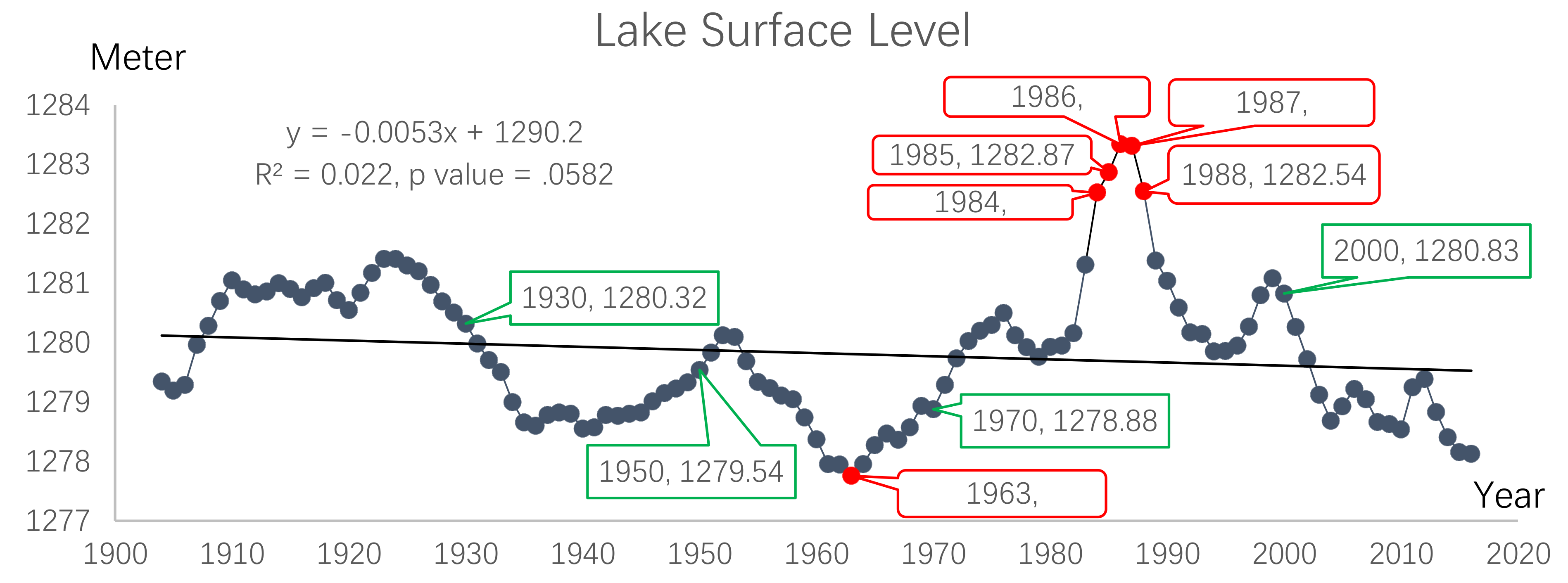
Table 1, but the 5th percentiles are all much larger than the lower bounds determined by mean—2SD. In other words, if the 95th percentile is used, there could be too many “extremely changing points” that in fact are not large enough to be extreme; while many more low values also can be added by using the 5th percentile, which are not small enough to be extremely low. Therefore, the 5th and 95th percentiles cannot make the extremely changing points as meaningful as it is defined to identify the extremely changing observations by using mean and 2SD. For instance, using the 5th and 95th percentiles, surface levels in 1923, 1924, and 1989 would be added as extremely high water levels to 1984, 1985, 1986, 1987, and 1988; surface levels in 1961, 1962, 1964, 1965, 2015, and 2016 would be added as extremely low observations in addition to 1963, as shown in
Figure 2. In other words, mean and 2SD are more robust and effective than the 5th and 95th percentiles to identify extreme values.
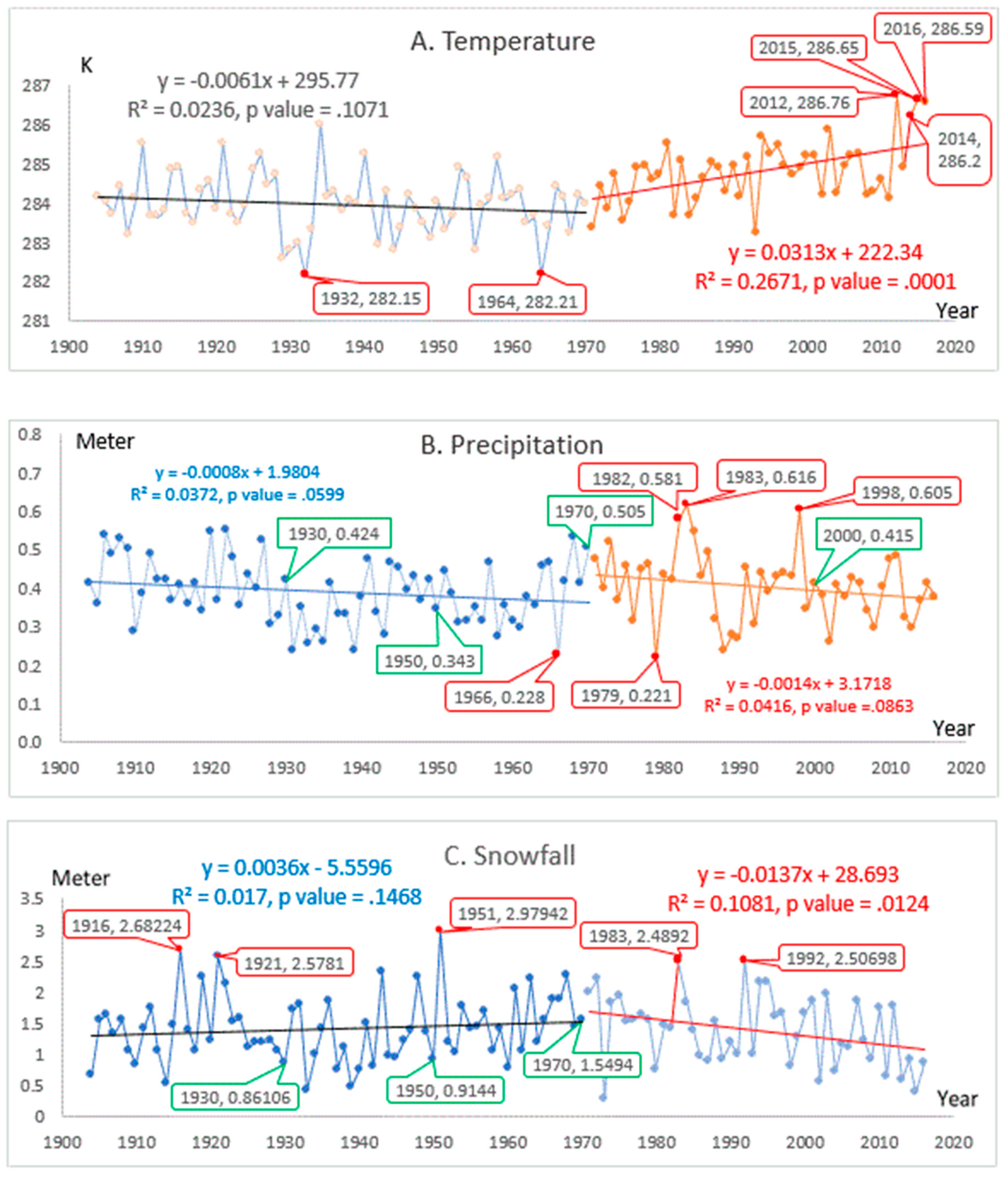
From the early 1970s, there is a significant trend of local climate warming in the GSL region, which is primarily driving the declines of the GSL, as shown in
Figure 3. Therefore, the climate variables of temperature, precipitation, and snowfall are analyzed into two periods, from 1904 to 1970 and 1971 to 2016, in which temporal trends are analyzed and extremely changing points are marked in red, as shown in
Figure 3.
Trend analysis is also applied to the lake surface level, temperature, precipitation, and snowfall in order to highlight the efficiency of extremely changing point analysis in hydrological and climate data analysis. For example, whether the GSL has a significant declining trend can be analyzed as a regression model with years as a predictor. If we use the lake surface level as an indicator of GSL declines, we need to regress the lake surface levels against years. The results of trend analysis and the extremely changing points are plotted and marked in red, as shown in
Figure 2 and
Figure 3.
3. Results and Discussions
In the last century, the GSL shows an apparent decreasing trend from 1904 to 2016 with the lowest level of 1277.76 meters in 1963, but its declining trend is not significant, as shown in
Figure 2. In other words, the significance of GSL declines is tested with a
p-value of 0.0582 that is just a little beyond the significance level 0.05. However, the periodic changes of its surface levels in both increasing patterns and decreasing patterns are anomalous in the last century, as shown in
Figure 2. This cannot be explained by the human water uses in agriculture, industry, and municipal purposes that were much lower in the last century than current days given the recently significant growth in agriculture, industry, and urbanization in the GSL basin. Instead, the GSL declines could be more clearly explained by climate change and extreme weather including both precipitation and temperature, which then are explained in the five sections below: local warming and evaporation, the impacts of radiation and wind on evaporation, precipitation, river discharge, and human water use.
3.1. Local Warming and Evaporation
Climate changes, especially increasing temperature, have caused significant water loss through evaporation in semi-arid regions [
12,
13,
14,
15,
16]. Craig et al. reported that increasing evaporation rates caused by climate warming have resulted in approximately 40% of Australia’s total water storage capacity loss every year [
16]. Helfer et al. and Johnson and Sharma obtained similar results of climate warming on evaporation, demonstrating that increasing temperature results in the significant increases of annual average evaporation [
13,
14,
15].
Specifically, Helfer et al. mentioned that a temperature increase range between 0.8 °C and 1.3 °C in 2030–2050 compared to 1990–2010 will result in an average annual evaporation from 1300 mm in 1990–2010 to an average annual 1400 mm in 2030–2050 [
13]; in other words, an annual temperature increase rate of 0.02 to 0.0325 would result in an average annual difference of 100 mm in evaporation. Additionally, an annual temperature increase rate of 0.021 to 0.04 would cause an average annual evaporation difference of 190 mm, i.e., evaporation from 1300 mm in 1990–2010 to 1490 mm in 2070–2090 caused by a temperature increase range of 1.7 °C to 3.2 °C in 2070–2090 [
13]. In the GSL region, the annual temperature increase rate is 0.0313 from 1971 to 2016, as shown in
Figure 3A. Given an average annual evaporation amount
E for the GSL before 1960 and the significant and consistent temperature increase from 1970 to 2016, as shown in
Figure 3A, the average annual evaporation in 1970–1990 could be
E + 100 mm, and the average annual evaporation in 2000–2020 could be
E + 190 mm. Therefore, the GSL has lost a huge amount of water from evaporation in the last 50 years. The extremely high temperatures in the recent years 2012, 2014, 2015, and 2016 directly aggravate the significant declines of surface water levels of the GSL due to the enhanced evaporation with the addition of low precipitation in the recent few years, and the GSL hence reaches a relatively low level of 1278.13 meters in 2016, as shown in
Figure 2 and
Figure 3. Therefore, evaporation and low precipitation are the main cause of the declines of the GSL.
3.2. Radiation, Wind Speed, and Evaporation
Some may still wonder if radiation and wind speed impact evaporation changes. Solar radiation increased significantly in the last century [
17], which indicated that evaporation increased too. The effects of wind speed on evaporation are complex. At low velocity values, the first stage evaporation rate will increase when wind speed increases, but at the same time the transition time decreases; however, at high values of wind speed, evaporation rates will depend less on the wind speeds; additionally, no significance is found for the impact of the wind speed on the second stage evaporation rate [
18]. In all, the effects caused by increasing radiation could be stronger than the effects of wind speed, and thus evaporation might increase in the last century; or the overall evaporation change caused by radiation and wind speed is not significant in the last century.
3.3. Precipitation
The temporal patterns of precipitation directly drive the general dynamics of GSL surface levels, which are then mainly modified by evaporation driven by temperature changes as discussed above. Both the periods from 1904 to 1970 and from 1971 to 2016 show apparent decreases in precipitation, but the significances are just above the significance level 0.05. Therefore, the declining trend of lake surface level is not quite significant. Since 1971 with about 10 years’ high precipitation, the GSL reached an extremely high level in 1984 that continued to 1988, as shown in
Figure 2, because of the extremely high precipitation in 1983, 1984, and the high precipitation in 1985 and 1986, as shown in
Figure 3. Additionally, from 1904 to 1930, the GSL surface levels were most often above its average value (1279.82 meters), as shown in
Table 1, because the precipitation in only 8 of 27 years was relatively lower than its average value of 0.395 meters, as shown in
Figure 3. In the 40 years from 1931 to 1970, only two year’s GSL surface levels (1952 and 1953) were relatively above its average level, because the precipitation in 27 years was much lower than the average precipitation, as shown in
Figure 3; especially with 20 more years of low precipitation, and in 1963, the GSL reached its lowest surface level (1277.76 meters) that was still above its extremely low level bound (1277.49 meters). From 1971 to 2000, there were only 9 of the 30 years when precipitation was less than its average value, and therefore most of the years the GSL surface levels were above its average level. The extremely high precipitation in 1998 resulted in the second highest surface level in 1999, as shown in
Figure 2 and
Figure 3. Although the precipitation in 1966 and 1989 was very low, respectively high precipitation following them continuously occurred for 7 or 8 years, which thus did not result in extremely low surfaces but relatively low water levels.
The continuously significant decreases in snowfall from 1971 to 2016 could be a secondary contribution besides the significant increasing temperature for the apparent declines of lake surface levels after 2000, as shown in
Figure 2 and
Figure 3. The extremely high snowfall in 1983 (2.489 m) also secondly contributed to the extremely high records of lake surface levels in 1984 to 1987.
3.4. River Discharge
Bear River, Jordan River, and Weber River are the major surface water discharges into the Great Salt Lake, which account for 58%, 22%, and 15%, respectively, for the total inflows of the lake [
2]. The U.S. Geological Survey (
https://waterdata.usgs.gov/) provides inflows from 1971 to 2018 for the Bear River and Joran River as displayed in
Figure 4 below, which have 80% of surface inflows for the GSL. Because the continuous data for Weber River are only available after 1989, it is not included into this decadal analysis. In general, the surface inflows show a significant declining trend, which contributes to the decreasing water level in the same period, as shown in
Figure 2. The reduced river discharge is directly caused by the declining precipitation and snowfall, as shown in
Figure 3.
The extreme highest points of the observed discharge values in 1983, 1984, 1986, as shown in
Figure 4, have significant contribution to the extremely high water levels, as shown in
Figure 2. These extreme highest values are also coincident to the extremely high precipitation values observed in 1982 and 1983. This is a truth that we first observed highest precipitation, secondly observed highest surface inflows, and third detected highest lake water levels. In the GSL basin, climate changes generally drive the river discharge patterns.
3.5. Human Water Use
We understand that human water use could be another secondary contribution to GSL’s water loss. However, the conclusion of ‘‘consumptive water use including agricultural, salt pond mineral production, and municipal and industrial uses rather than long-term climate change has greatly reduced its size for the Great Salt Lake’s surface declines’’ [
2], cannot explain the much lower surface levels in 1961, 1962, 1963, and 1964 that were lower than 2016’s current record, the significant declines from the early 1920s to the late 1930s, the significant increasing trend from the mid-1960s to the mid-1970s, and other significant declining or increasing patterns in the last century, as shown in
Figure 2.
Additionally, human water use even cannot explain the current GSL water level changes in 2016, 2017, and 2018, as shown in
Figure 5. The average water levels in 2017 or 2018 are 0.91 meters higher than that in 2016. If human water use was the dominant driving force for GSL water loss or dynamics, it is impossible that in three continuous years, significantly less human water use has occurred, which then has resulted in such a huge amount of water increases in 2017 or 2018. Another recent study also showed worldwide declines of water storage in endorheic basins in the last 10 more years were caused by limited precipitation with high potential evaporation, which are then intensified by global warming and human activities [
19]. Thus, human water use is not the dominant cause but could be a secondary factor of saline lakes’ water loss.
3.6. Correlation between Temperature, Precipitation, Snowfall, River Discharge, And Gsl Water Level
The above analyses have showed apparent temporal patterns of temperature, precipitation, snowfall, and river discharge. Chang and Bonnette have recently examined the correlation between climate and water-related ecosystem services [
20]. Here, we use the Pearson correlation coefficient to quantify a general relationship between temperature, precipitation, snowfall, river discharge, and GSL water level, as shown in
Table 2. From 1971 to 2016, the significant increasing temperature is significantly and negatively related to GSL water levels. It coincides with the above analysis that local climate warming is a critical variable for water loss. Another significant relationship is between GSL water levels and river discharge. River discharge is significantly and highly correlated with precipitation, as shown in
Figure 6, which further indicates that climate factors, especially precipitation along with temperature, are the dominant driving force of GSL water level dynamics.
4. Limitations
Many other studies recently have showed that the GSL water levels are primarily sensitive to climate cycles, given its main outflow is evaporation that is directly changed by lake area and salinity, and precipitation variations mainly drive the GSL water level variation [
20,
21,
22]. Rather than following the previous research approaches, this proposed study, based on a simple water balance equation of inflow and outflow, explored how climate and weather factors could impact on inflow and outflow, and concluded that climate change and local extreme weather drive the dynamics of GSL water levels. This is not the primary objective of this short communication; we hope this short communication could encourage more high quality studies and inspire scientists to rethink water budget modeling, climate modeling, and hydroclimatological analysis, so that the driving force of water dynamics of salt lakes could be truly modeled and quantified, which then will provide useful and practicable information for water budget planning and water resources management.
We understand that there are many sophisticated models for climate and hydroclimatological analyses, but “all models are wrong, and some are illuminating and useful” [
23,
24]. Scientists cannot achieve a “correct” model by excessively elaborating modeling procedures and parameters; while for great scientists it is significant to devise simple and evocative models, any overelaboration and over-parameterization is nothing but mediocrity [
23,
24]. There are some limitations in this short communication. For example, we do not directly examine the impacts of human water use on water level dynamics of GSL, while we analyze the remaining factors for water balance including inflow factors (i.e., precipitation, snowfall, and river discharge) and outflow factors (i.e., evaporation, temperature) that influence the water levels of GSL. We do not have direct measurements of evaporation in the GSL region, but evaporation estimations of water bodies of similar semi-arid regions in Australia are referenced to indicate the impacts of evaporation on GSL water loss. Long-term surveys of evaporation and measurement of human water use can be helpful in order to further analyze and quantify the primary and secondary factors driving the dynamics of saline lakes. Additionally, the 95th and 5th percentiles cannot effectively identify extremely high or low observations of water levels, precipitation, temperature, and snowfall, which further indicates our proposed extremely changing point analysis with mean and two standard deviations is a robust and promising method for hydroclimatological analysis.
5. Conclusion
The proposed temporal trend with the extremely changing point analysis is a promising method to clearly and concisely define and understand the characteristics of extreme climate/weather and their impacts on the declines of saline lakes. Extremes have become foundational information and projections for climate change, which has been highlighted 734 times in the current US Global Change Research Program’s Climate Science Special Report [
25]. Most often, an explicit definition of extreme is not provided in current research and management, but clearer definitions and quantifications of extremes can support interdisciplinary understanding and decision making of extreme events [
6]. Defined by whether an observation is outside its two standard deviations of the mean, the extremely changing points indicate the substantial changes of a variable in its temporal patterns. Using the proposed temporal trend with extremely changing point analysis, this short communication adequately shows that climate change and extreme weather can be the primary driving factors of the dynamics/declines of the Great Salt Lake. Although the impact of one isolated extremely changing point could be limited, two more continuously or clustered extremely changing points can have elevated impacts on the environment. For example, extremely high temperature in 2012, 2014, 2015, and 2016 considerably enhances the continuously increasing evaporation of the GSL since the 1970s. The extremely low precipitation in 1979 is isolated, and therefore its effect was minimized by many of those much higher precipitation observations neighboring and close to it.
Climate changes, especially local warming and extreme weather including both precipitation and temperature, drive the dynamics of the GSL surface levels. Extreme weather, such as extremely high or low precipitation, directly causes the changes in surface levels, and the extremely high temperature in the last five years has resulted in much more water loss through evaporation that can be another main cause of the relatively low surface level in 2016. The increasing temperature trend since the 1970s, as shown in
Figure 3, has become a critical role in water loss and hence the decline of the GSL surface levels. As discussed above, many studies have proven that climate warming has resulted in the main water loss through evaporation (i.e., each year about 40% of the total water storage capacity in Australia). The annual increasing rate of 0.0313 in temperature from 1971 to 2016 could result in more than 40% loss of its total water storage each year.


