Decadal Oscillation in the Predictability of Palmer Drought Severity Index in California

Abstract

Severity of drought in California (U.S.) varies from year-to-year and is highly influenced by precipitation in winter months, causing billion-dollar events in single drought years. Improved understanding of the variability of drought on decadal and longer timescales is essential to support regional water resources planning and management. This paper presents a soft-computing approach to forecast the Palmer Drought Severity Index (PDSI) in California. A time-series of yearly data covering more than two centuries (1801–2014) was used for the design of ensemble projections to understand and quantify the uncertainty associated with interannual-to-interdecadal predictability. With a predictable structure elaborated by exponential smoothing, the projections indicate for the horizon 2015–2054 a weak increase of drought, followed by almost the same pace as in previous decades, presenting remarkable wavelike variations with durations of more than one year. Results were compared with a linear transfer function model approach where Pacific Decadal Oscillation and El Niño Southern Oscillation indices were both used as input time series. The forecasted pattern shows that variations attributed to such internal climate modes may not provide more reliable predictions than the one provided by purely internal variability of drought persistence cycles, as present in the PDSI time series.

1. Introduction

Drought is a fundamental feature of the climate of North America, where several regions of western United States (U.S.) have experienced protracted decadal-scale dry periods in the past centuries [1] Hydrologic droughts in western U.S. were already widespread and persistent during the so-called Medieval Climatic Anomaly, roughly in the period 900–1300 AD [2], with mega-drought in southern California during 832–1074 AD and 1122–1299 AD [3,4]. Multi-year droughts have also recurred in more recent times, e.g., in 1818–1824, 1827–1829, 1841–1848 and 1855–1865 (Figure 1), causing tremendous disruption on social, agricultural, ecological and economic fronts [5]. Five major droughts followed, which ended in 1924, 1935, 1950, 1960 and 1977. As well, the one started in 2012 [1] resulted in statewide proclamations of emergency [6]. Much of the water supply for California is derived from the Sacramento-San Joaquin River Delta (located in Northern California) via pumps located at the southern end of the delta. However, in recent times, California’s water resources have been subject to increased stress from a combination of factors including a growing population, groundwater deficit, limitations on extraction of water for the protection of fish, and increased competition for available water [6]. Over 2012–2016, drought conditions impacted surface water supplies, and increased agricultural demand and land subsidence owing to groundwater extraction. These factors inspired the development of legislation to regulate groundwater resources and financially support sustainable groundwater management as well as cleanup and storage [7]. Water management in the state (which has been studied extensively [8]) shows that the California case is exemplary of the preparedness and response measures required to cope with extreme drought events, adapt to them and build long-term resilience [9]. How drought may change in future is of great concern as global warming continues [10]. Yet, how has an extreme drought occurrence over California shifted as a result of the change in climate since historical times? How can we see droughts coming? If we are dry during one drought year, will we likely be dry for other drought years, and then for a decade or more? How cyclical will these patterns be and how are they predictable over multidecadal time-scales? To answer these questions, we examined (with focus on California) uncertainties in estimating the future ramifications of years of drought, and how drought changes may recur in the near future using the Palmer Drought Severity Index (PDSI).

Many of drought indices developed for the purpose of drought monitoring are based on meteorological and hydrological variables, which show the size, duration, severity and spatial extent of droughts. The Palmer Drought Severity Index (PDSI) is such an example. Originally developed by Palmer [11], it is one of the most well-known and widely used drought indices in the U.S. [12,13] and beyond [14,15,16,17] PDSI values are computed along the soil moisture balance that requires time series of temperature, precipitation, ground moisture content (or available water-holding capacity) and potential evapotranspiration. The calculation algorithm of PDSI—either in its original version by Palmer [11] or in modified ones [18] is thus a reflection of how much soil moisture is currently available compared to that for normal or average conditions. The PDSI incorporates both precipitation and temperature data in a simplified, though reasonably realistic, water balance model that accounts for both supply (rain or snowfall water equivalent) and demand (temperature, transformed into units of water lost through evapotranspiration), which affect the content of a two-layer soil moisture reservoir model (a runoff term is also activated when the reservoir is full). Not explicitly bounded, the PDSI typically falls in the range from −4 (extreme drought) to +4 (extremely wet). The PDSI is a dimensionless quantity for comparison across regions with radically different precipitation regimes. This means that there are limitations in the use of this index at specific scales, for which other drought indices have been developed to characterize local agricultural and socio-economic contexts [19].

Land-atmosphere interactions can introduce persistence into droughts because reduced precipitation lowers soil moisture, reduces surface evapotranspiration and, with less vapor in the atmosphere, further reduces precipitation. In this sequence, soil moisture adjustment occurs with a length of time, which introduces a lag and a memory. Depending on situations, there might be a strong coupling between soil moisture and precipitation, and land surface processes can lead to persistence [20]. The calculation of PDSI is intended to model soil moisture persistence (or memory). The combination of past wet/dry conditions with past PDSI data means that the PDSI for a given time step (generally one month) can be seen as a weighed function of current moisture conditions and a contribution of PDSI over previous times [21]. In the light of this persistence structure, PDSI chronologies can be used to reconstruct drought conditions, but persistence can also be a criterion to be used as a measure of predictability [16].

This paper deals with time series analysis (TSA) related to PDSI dynamics. Several statistical TSA approaches were applied to predict climate variables, including their extremes [22,23]. Mossad and Alazba [24] proved the potential ability of these modelling approaches to forecast drought. However, drought forecasts performed at monthly time-scale for early warning [25,26,27,28,29] do not account for long-term patterns of evolution, which are essential to study and monitor drought from a climate perspective [30]. Here, we target annual to decadal time scales. We investigate to what extent TSA model simulations may provide reliable forecasts of future hydrological changes. Although research on meteorological drought (that is, when dry weather patterns dominate) is particularly difficult because of the complex and heterogeneous character of drought processes, their temporal trends respond to climate fluctuations (e.g., large-scale atmospheric circulations). Specifically, the work explores a homogenized long series of annual PDSI data (1801–2014) as derived for California by Griffin and Anchukaitis [1] and accessible at https://www1.ncdc.noaa.gov/pub/data/paleo/treering/reconstructions/california/griffin2015drought.txt (identifier ‘precip-ONDJFMAMJ-rec-2rmse’, providing precipitation anomalies serving as reasonable proxy of PDSI data taken at the lower limit of twice the root mean square error). Then the study assesses the response of an exponential smoothing (ES) model, using an ensemble prediction approach. ES [31,32] and autoregressive integrated moving average (ARIMA) models [33] are the most representative methods in TSA. In this study, ES was used because it is known to be optimal for a broader class of state-space models than ARIMA models [32]. ES responds easily to changes in the pattern of time series [34] and is often referred to as a reference model for time-pattern propagation into the future [35,36]. It is also less complex in its formulation and, as such, it was expected to be easier in identifying the causes of unexpected results. The ensemble approach has been adopted as a way to consider uncertainty in hydrological forecasting, and thus enhance accuracy by combining forecasts made at different lead times, as in Armstrong [37] and in previous authors’ papers [38,39,40,41]. A lengthy PDSI series offers a unique opportunity to explore past interannual-to-interdecadal climate variability, under the assumption that the past interannual climate variability, with its internal dependence structure, can be used to replicate future PDSI ramifications at the local scale. This approach was compared with the more traditional TSA approach using transfer function models (TFM), introduced by Box and Jenkins [42] and re-visited by Shumway and Stoffer [43]. In this case, input time series of El Niño Southern Oscillation (ENSO) and the Pacific Decadal Oscillation (PDO) were considered as impulse inputs to the output PDSI time series. An approximate ensemble approach was also developed under the transfer function models (TFM) framework for comparison purposes with the ES results. For California, there are now accessible accurate long-time series of PDSI. Our focus is motivated because severe and widespread drought are of particular concern for this U.S. state [44].

2. Materials and Methods

2.1. Environmental Setting and Data

The California’s climate varies widely, from hot desert to subarctic, depending on latitude, elevation, and proximity to the coast. California’s coastal regions, the Sierra Nevada foothills, and much of the Central Valley have a Mediterranean climate, with warm to hot, dry summers, and mild, moderately wet winters (Figure 2a,b). The influence of the ocean generally moderates temperature extremes, creating warmer winters and substantially cooler summers in coastal areas. The rainy period in most of the country is from November to April (Figure 2a). Prevailing westerly winds from the Pacific Ocean also bring moisture. The average annual rainfall in California is about 350 mm, with the northern parts of the state generally receiving higher rain amounts than the south. The reference evapotranspiration follows a more complex pattern, mostly in relation to elevation and distance from sea (Figure 2c). Temperature and evapotranspiration are especially important in California, where water storage and distribution systems are critically dependent on winter/spring rainfall, and excess water demand is typically met by groundwater withdrawal [45]. The PDSI time series derived from Griffin and Anchukaitis [1] reconstructed drought conditions for California.

2.2. Exponential Smoothing

The exponential smoothing (a popular scheme to produce smoothed time series) is a relatively simple prototype model for TSA-based forecasting, analysis and re-analysis of environmental variables [46,47]. It uses historical time series data under the assumption that the future will likely resemble the past, in an attempt to identify specific patterns in the data, and then project and extrapolate those patterns into the future (without using the model to identify the causes of patterns). Compared to other techniques (e.g., moving averages), which equally weight past observations, exponential smoothing apportions exponentially decreasing weights as observations get older. This means that recent observations are given relatively more weight in forecasting than older observations. To compute predictions based on the observed time series of PDSI data, we made use of available knowledge concerning the period of the system under investigation [48]. The following periodic simple exponential smoothing [35] was selected as reference model for time-pattern propagation into the future:

$$F{\left(X\right)}_{t+m}^R=\alpha ·\frac{S_t}{I_{t-p}}$$

(1)

where $F{\left(X\right)}_{t+m}^R$ represents the m-step-ahead forecast from the annual series of the variable X (PDSI) on N years for an ensemble of R runs; S_t is the smoothed PDSI at decadal scale centered on time-year t (Equation (2)); α is the smoothing parameter for the data; I_t−p is the smoothed cycle index at the end of period t, its number being defined by the periods p in the seasonal cycle (Equation (3))

$$S_t=\alpha ·\frac{X_t}{I_{t-p}}+\left(1-\alpha \right)·S_{t-1}$$

(2)

$$I_{t-p}=\delta ·\frac{X_t}{S{\left(X\right)}_t}+\left(1-\delta \right)·I_{t-1}$$

(3)

where δ is smoothing parameter for cyclical indices.

2.3. Transfer Function Models

Results from seasonal exponential smoothing (that uses the temporal dependence structure of the time series itself to reproduce the time series behavior in the future) were compared to an alternative methodology based on transfer function models (TFM). It represents a linear transfer function approach where input time series potentially impacting the drought behavior at large spatial scales are used as explanatory time series variables in a lagged regression model. The methodology called TFM was introduced by Box and Jenkins [25] and re-visited by de Guenni et al. [49] and Shumway and Stoffer [43] (2017) to forecast monthly rainfall in the coast of Ecuador based on El Niño indices and model the impact of El Niño on fish recruitment, respectively.

In a TFM, the output series (in this case PDSI) can be represented as:

$$Y\left(t\right)={\alpha }_1\left(B\right)·X_1\left(t\right)+{\alpha }_2\left(B\right)·X_2\left(t\right)+\dots +{\alpha }_k\left(B\right)·X_k\left(t\right)+\eta \left(t\right)$$

(4)

where X₁(t), X₂(t), …, X_k(t) are the input time series to be considered as explanatory variables contributing to the temporal dynamics of the output series Y(t) and η(t) is a stationary random process. The terms α₁(B), α₂(B), …, α_k(B) are fractional polynomials in the back-shift operator B (such that B^S(X(t) = X(t − s)) of the form:

2.4. Model Validation Methods

To ensure the optimal runs over the hold back prediction (testing validation), model parameterization was achieved by minimizing together the Root Mean Squared Error (RMSE) and the Mean Absolute Scaled Error (MASE), and maximizing the correlation coefficient (R). The commonly used RMSE quantifies the differences between predicted and observed values, and thus indicates how far the forecasts are from actual data. A few major outliers in the series can skew the RMSE statistic substantially because the effect of each deviation on the RMSE is proportional to the size of the squared error. The overall, non-dimensional measure of the accuracy of forecasts MASE [50] is less sensitive to outliers than the RMSE. The MASE is recommended for determining comparative accuracy of forecasts [51], because it examines the performance of forecasts relative to a benchmark forecast. It is calculated as the average of the absolute value of the difference between the forecast and the actual value divided by the scale determined by using a random walk model (naïve reference model on the history prior to the period of data held back for model training). MASE < 1 indicates that the forecast model is superior to a random walk. The correlation coefficient between estimates and observations [52] (anti-correlation) (perfect correlation)—assesses linear relationships, in that forecasted values may show a continuous increase or decrease as actual values increase or decrease. Its extent is not consistently related to the accuracy of the estimates. WESSA R–JAVA web [53] was used to assess model simulations with spreadsheet-based support.

In order to quantify long-range dependence and appraise the cyclical-trend patterns in the series, we estimated the Hurst [54] H exponent (rate of chaos), which is related to the fractal dimension D = 2 − H of the series. Long memory occurs when 0.5 < H < 1.0, that is, events that are far apart are correlated because correlations tend to decay very slowly. On the contrary, short-range dependence 0.0 < H < 0.5 is characterized by quickly decaying correlations, i.e., past trends tend to revert in the future (an up value is more likely followed by a down value). Calculating the Hurst exponent is not straightforward because it can only be estimated and several methods are available to estimate it, which often produce conflicting estimates [55,56]. Using SELFIS (SELF-similarity analysis [55], we referred to two methods, which are both credited to be good enough to estimate H [57]: the widely used rescaled range analysis (R/S method) [58], and the ratio variance of residuals method, which is known to be unbiased almost through all Hurst range [59]. Long-memory in the occurrence of PDSI values was also analyzed to see if the memory characteristic is correlated with the length of the time series. To determine whether this characteristic changes over time, the Hurst exponent was not only estimated for the full time series (1801–2014), but also for a shorter series starting in 1901 (the most recent period, which is also the period held out of the calibration process).

3. Results and Discussion

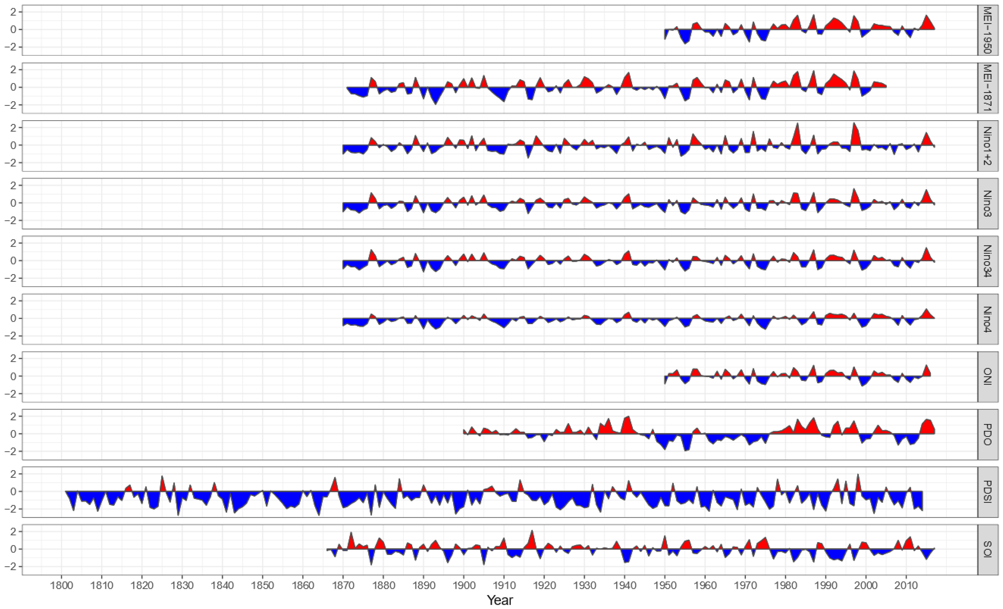
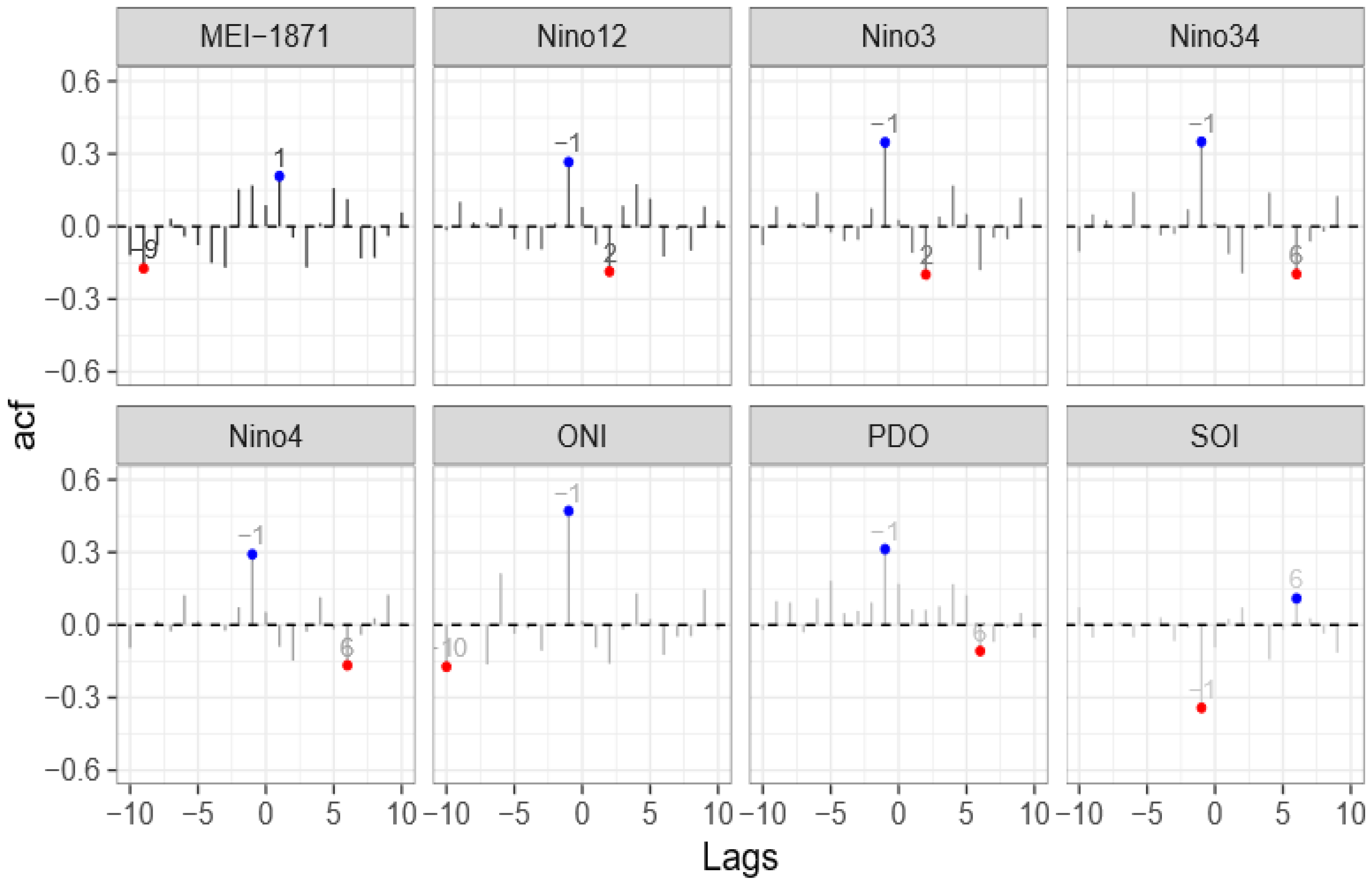
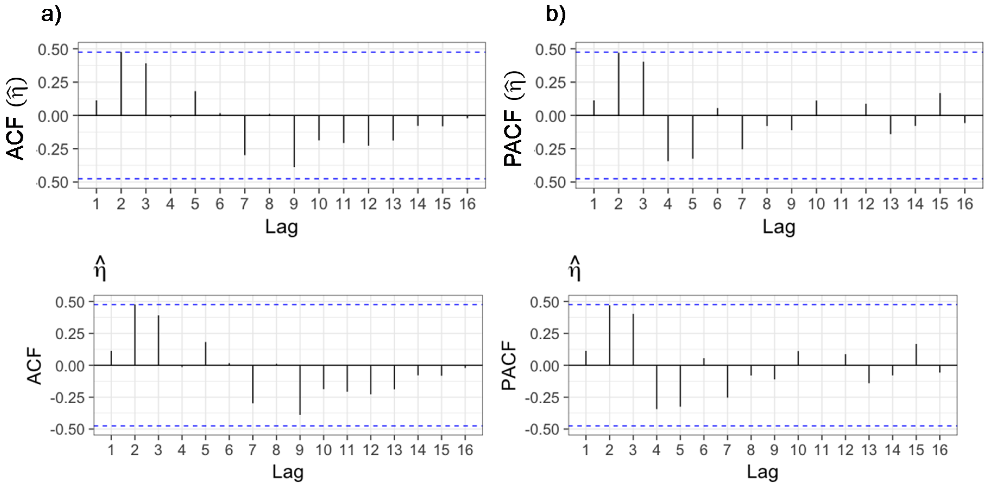
3.1. Data Analysis

The first step in any time-series analysis and forecasting is to plot the observations against time, to gain an insight into possible trends and/or cycles associated with the temporal evolution of datasets. Figure 3a shows that the PDSI time series presents important inter-annual and decadal variability, with smooth changes in its structure and turning points which help in orienting the choice of the most appropriate forecasting method [60]. Two homogeneity tests indicate a stepwise shift in the observational series in the years just before 1920. The Buishand range test [61] places the change point in 1969, whereas the Mann-Whitney-Pettitt test [62] locates it in 1920 but the two tests are not significant (p > 0.10), from which the series can be considered as relatively stationary.

The smoothed periodogram of the PDSI time series (Figure 4) was calculated by using the smoothing method [63] implemented in the R software [64] This estimate shows that most of the total variability in the series is associated with both short and large frequencies. The multiple observed maxima in the power spectrum confirm the complex interactions of several physical drought-triggering processes acting at several time scales. The maximum estimated spectral density occurs at frequency 0.185, which corresponds to a cycle of 5.4 years [65]. This cycle might be associated with El Niño phenomenon, but other frequencies have also an important contribution to the overall series variability.

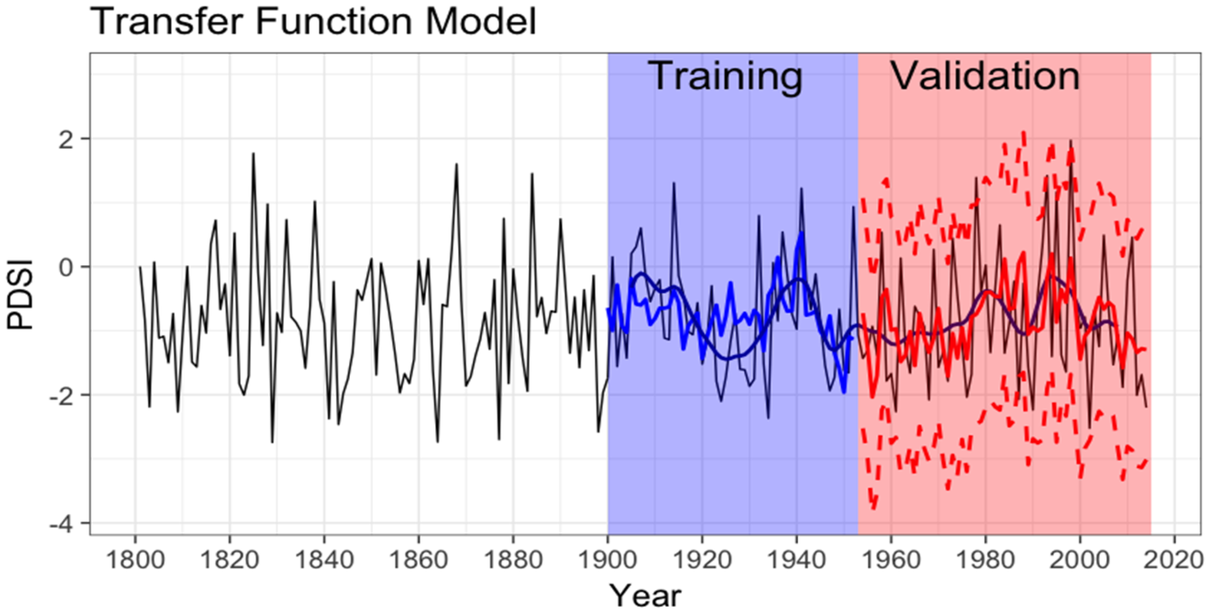
3.2. Validation Results and PDSI Time Series Predictability

The whole of the PDSI time series (214 years of data from 1801 to 2014) was segregated into sub-sets for the purposes of training and validation (Figure 3a). The choice of 1801 as starting time of the series was driven by the necessity of having a sufficient amount of data for training without laying too long back in time, considering that with at least 50 observations are necessary for performing time-series analysis/modelling [66]. On the other hand, with at least 150–200 observations potentially reliable forecasts can be obtained for 30 to 50 steps ahead [67]. Forecasts were performed for the 40-year follow-up period (Figure 3b). Alternative initial conditions were simulated for each run, taking periods with a different start year (in 10-year steps-up from year 1801 to 1900) and periodical cycles (41, 42 and 43 years) for model training (training datasets).

For 1954–2014 (Figure 3b), the simulation results for validation testing are quite promising, judging by the closeness of ensemble prediction mean (red curve) to the observed 11-year Gaussian Filter (black curve) PDSI evolution. The results indicate that the ES model performs well at both high and low frequency variability, which is consistent with inter-annual to inter-decadal climate-variability. In fact, the residuals between predicted and observed time-series are coherent in the validation period: residual histograms and Q-Q plots do not identify substantial departures from normality in both the official run with the longest training time (Figure 5a,a1) and the average (ensemble mean) of all the runs (Figure 5b,b1).

The data are somewhat right-skewed; however, the right tail of the distribution is fairly closely approximated by the normal distribution, with some high extreme values.

In the validation stage, RMSE and MASE were equal to 1.0 and 0.68, respectively, which indicate a satisfactory performance, and that the forecast model is superior to a random walk. The estimated Hurst (H) exponent values are reported in

Table 1. Estimated values of the Hurst (H) exponent (with two methods) for the PDSI annual series as a whole and for a reduced number of years.

Hurst (H) Exponent/Estimation Method	Whole Series (1801–2014)	Reduced Series (1901–2014)
Rescaled range (R/S)	0.611	0.743
Ratio variance of residuals	0.611	0.550

.

With the R/S method, the H was found to be greater than 0.6 in both the whole series (0.611) and the sub-set 1901–2014 (0.743), which is around the threshold of 0.65 used by [68] to identify series than can be predicted accurately. In the case of the variance of residuals method, we have a situation in which obtained results are hard for interpretation. With an increase of the number of series terms (amount of observations), the Hurst exponent is expected to get closer to 0 [69], i.e., the memory effect decreases. However, with the variance residuals method, the estimated Hurst exponent moves away from 0.5 with the whole of the time series (0.611 against 0.550 with the sub-set 1901–2014). These apparently contradictory results can be reconciled by considering that a complex concept such PDSI is hardly captured by one metric, the Hurst exponent, which (depending on the estimation method used) may not reflect the changes of heading direction [70]. Indeed, the whole of the series (Figure 3a) shows frequent and sudden pulses of drought, with a change-point in 1917, as identified by the Buishand test [61], observed in coincidence with the early 20th century pluvial centered on 1915, which has received much attention in the western U.S. [21]. By combining these results, it can be stated that the California’s PDSI series is related with either a short-range or a long-range memory (in turn reflecting influences on the occurrence of droughts of both large-scale and small-scale climate systems), which assumes that some dependence structure exists that advocates the foreseeability of the series. We thus performed our forecasting analysis on the original time series of PDSI data.

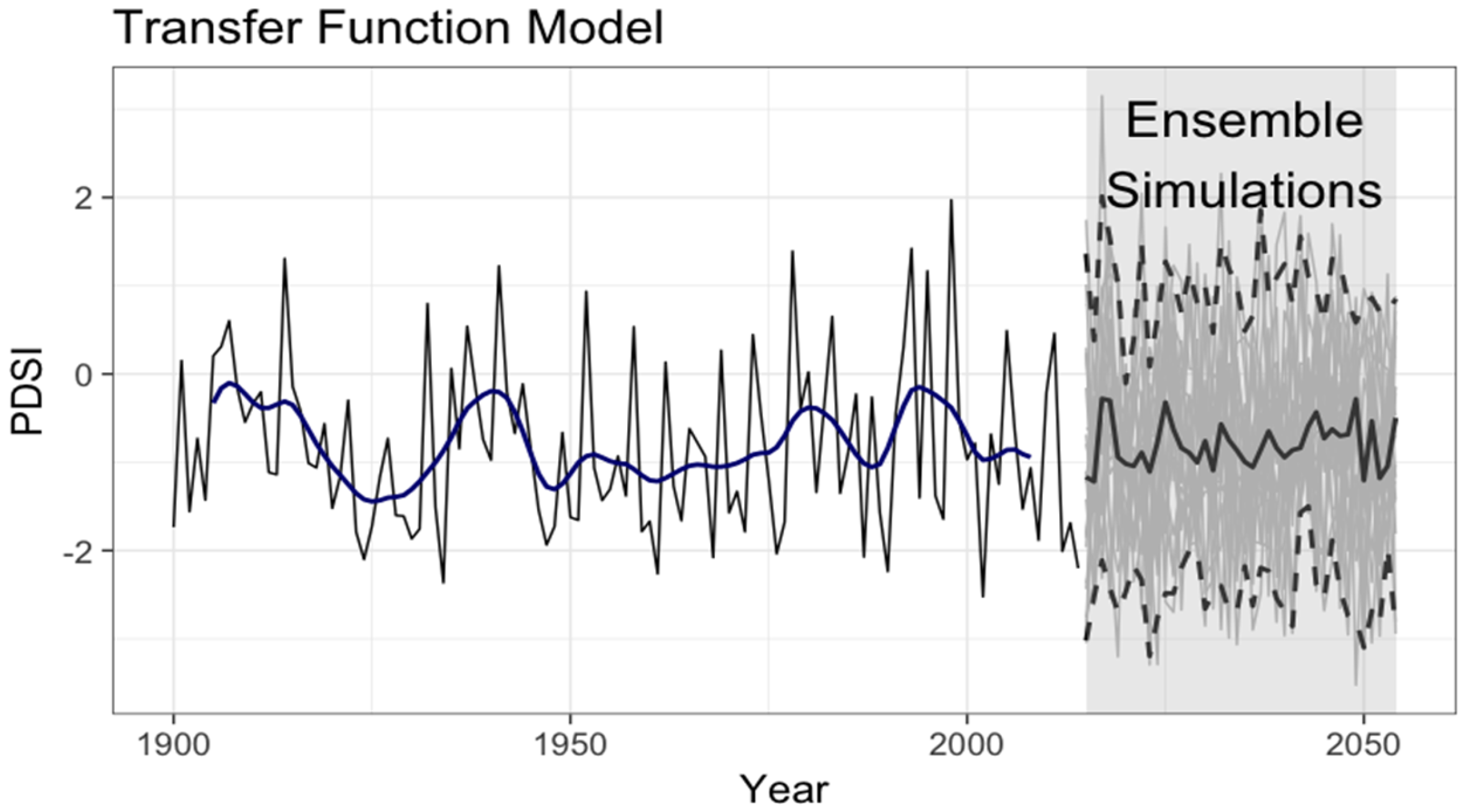
3.3. Simulation Experiment

Once the performance of the ES model was established, the model trained over 1801–2014 periods was run to produce an ensemble of forecast paths of annual PDSI for 2015–2054. Our major interest was directed towards assessing the predictability of interdecadal variations. Several forecast members show for the coming decades (Figure 6) some trajectories following a cyclical pattern, in which PDSI may fall below and above “incipient drought”, with negligible monotonic, long-term trend. However, moving forward, ongoing changes in atmospheric circulation and associated precipitation and temperature variability in the western U.S. raise questions about the stationarity of extreme drought estimates [71].

When examining the projection of PDSI over four future decades (2015–2054), the ensemble mean value (Figure 6, black bold curve) is observed to roughly lie around the “incipient drought” class, approaching “mild drought” around 2030, although some members push to “extreme drought”. Around 2020 and 2036, PDSI forecasts approach “near normal” with some members which are inclined up to “incipient wet spell”. After the year 2040, the PDSI resumes decreasing and remains below the “incipient drought” for years.

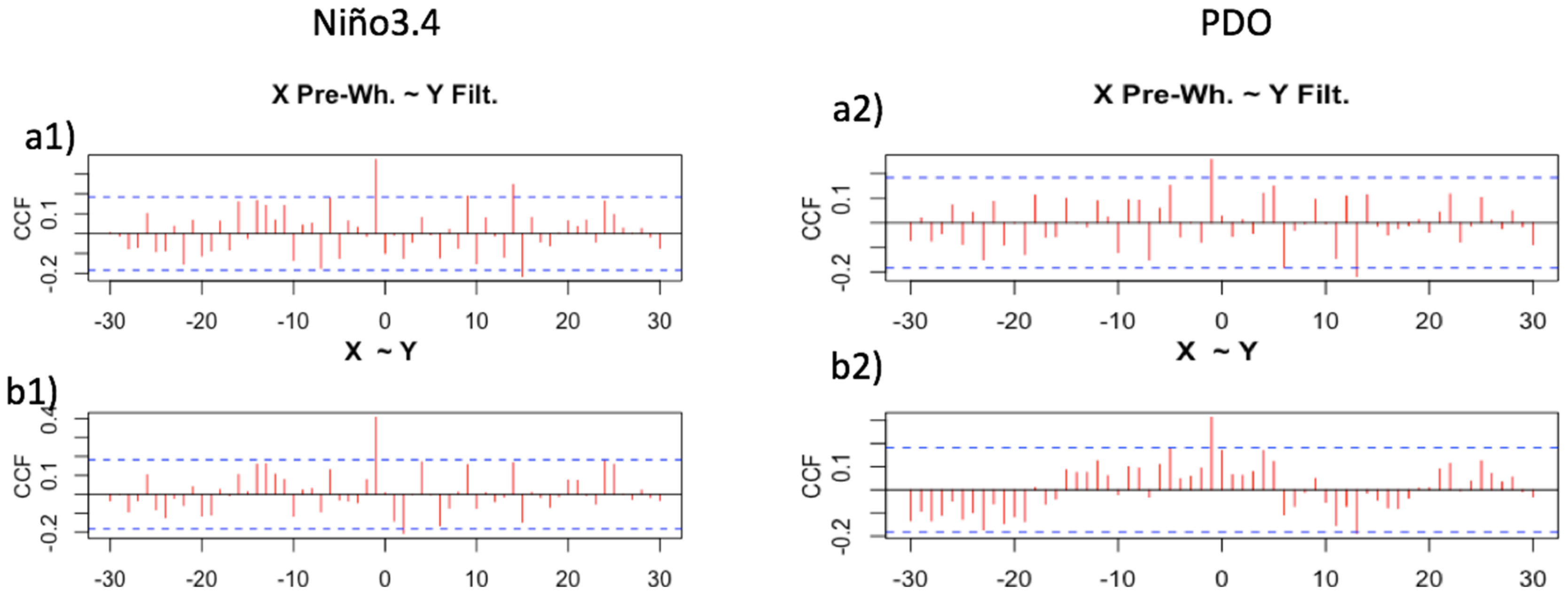
3.4. Comparison with the Transfer Function Modelling Approach

The band of warm ocean water that develops inter-annually in the central and east-central equatorial Pacific, El Niño Southern Oscillation (ENSO), is the major source of climate variability affecting different parts of the world [72,73]. However, the Pacific Decadal Oscillation (PDO), i.e., the variation of sea surface temperatures in the Pacific Ocean north of 20° N with a warm phase and a cool phase can modulate the interannual relationship between ENSO and the global climate [74]. The teleconnection of precipitation in California with climate phases such as the PDO and ENSO are reported in literature. A warm (positive) PDO is thought to have a similar spatial precipitation signature as a positive ENSO (wet in the American Southwest and dry in the Pacific Northwest), and a cool (negative) PDO has a similar signature as a negative ENSO [75]. ENSO has an important influence on the rainfall regime in California and most of the U.S. with most dramatic impacts during the winter season [76]. The PDO is also relevant because its cool phase is linked to dry conditions in Southern California and neighboring states [77]. A plot of all available ENSO time series jointly with the PDO and PDSI time series is shown in Figure 7.

Sample cross-correlation functions (Figure 8) show that, among all ENSO indices, the ONI series produced the highest cross-correlation with the PDSI series at a lag of −1 (=0.43), with the ONI series leading by one time step (one year) the PDSI series. However, since this series is rather short (available from 1950 onwards), we selected the next highly correlated series with PDSI, i.e., el Niño3.4 index (=0.35 at lag −1), with the Niño3.4 series leading the PDSI series. Since the PDO time series is available from year 1900, this was considered the initial year for the analysis. The model training period was the interval 1900–1953 and the model validation period was the interval 1954–2014. The latter coincides with the validation period used for the ES approach (Section 3.3). An ARIMA model was fitted to the PDO series for the training period. An autoregressive model of order 1 (AR(1)) was adequate for the series. Figure 9a2 presents the sample cross-correlation function (CCF) between the PDO series (X) and the PDSI series (Y), and the sample CCF between the pre-whitened X series (residuals after fitting an ARIMA model), with the filtered Y series (after applying the AR(1) filter) presented in Figure 9a1).

Similarly, an ARIMA model was fitted to the El Niño3.4 series for the training period. An autoregressive model of order 2 (AR(2)) was adequate for the series. Figure 10b₁ presents the sample cross-correlation function (CCF) between El Niño 3.4 series (X) and the PDSI series (Y), and the sample CCF between the pre-whitened X series (residuals after fitting an ARIMA model) and the filtered Y series (after applying the AR(2) filter) in Figure 10b₁. Figure 9b1,b2 show a significant spike at lag = −1 for the CCF between Niño3.4, and PDSI series and PDO and PDSI series. After filtering the input and output time series to discard the autocorrelation effects, Figure 9a1,a2 show the persistent significant leading impact of the Niño3.4 and the PDO series on the PDSI series one year in advance (lag = −1). From the sample CCF functions and according to Box and Jenkins [42], a transfer function model of order $\left(r_1,s_1,d_1\right)=\left(1,1,1\right)$ for input series $X_1\left(t\right)$ = Niño3.4, and order $\left(r_2,s_2,d_2\right)=\left(1,0,1\right)$ for input series $X_2\left(t\right)=PDO$, was proposed for this data set. In this case ${\alpha }_1\left(B\right)=\left({\delta }_{01}+{\delta }_{11}B\right)B^1/\left(1-{\omega }_{11}{B}^1\right)$ and ${\alpha }_2\left(B\right)=\left({\delta }_{02}\right)B^1/\left(1-{\omega }_{12}{B}^1\right)$.

The final model to be fitted is of the form:

$$Y_t={\alpha }_1{Y}_{t-1}+{\alpha }_2{Y}_{t-2}+{\alpha }_{3}Nino{3.4}_{t-1}+{\alpha }_{4}Nino{3.4}_{t-2}+{\alpha }_{5}PD{O}_{t-1}+{\eta }_t$$

(5)

Following Shumway and Stoffer [43], this model was initially fitted by least squares and the ARIMA model associated to the estimated residuals $\eta$ was identified. As a second step, the model was refitted assuming autocorrelated errors following an ARIMA model with order identified in the previous step. Figure 10 shows the autocorrelation and partial autocorrelation function of the estimated residuals, suggesting a white noise structure with no additional refitting required.

Figure 11 compares the observed values (black line) with the fitted values for the training period (blue line) and the observed values with the fitted values for the validation period (red line). The 95% prediction intervals are also shown in the analysis.

RMSE = 1.0 and MASE = 0.95 during the validation period indicate that the TFM provided an improvement over the naive forecast. Considering that in this case the training period (1900–1953) is much shorter in comparison with the training period used for the ES method (1800–1953), the TMS provides a competitive approach as a forecasting method for the PDSI series. The histogram and Q-Q plots of the residuals between the predicted and observed values for the PDSI time series during the validation period shows a satisfactory performance with an approximate normal distribution of the residuals (Figure 12).

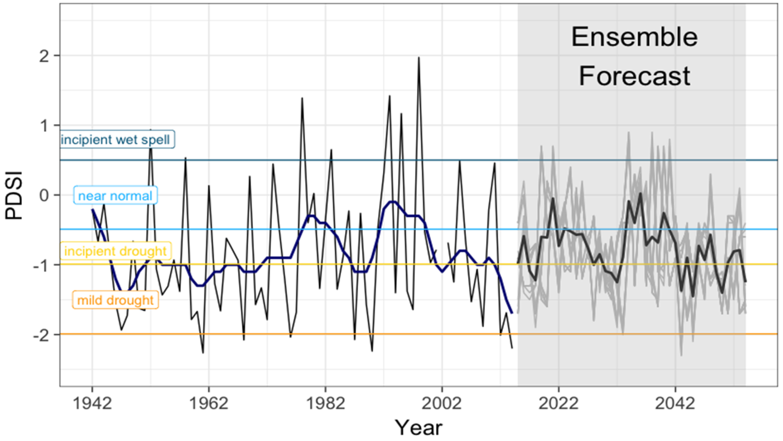
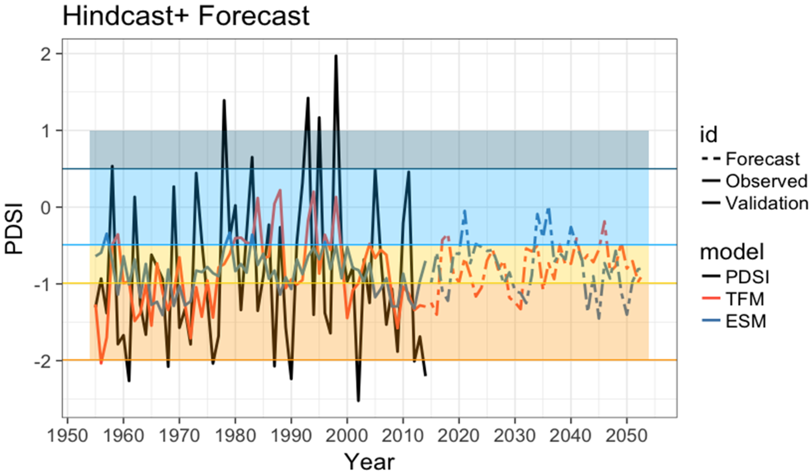
3.5. Ensemble Forecast with the Transfer Function Model

Once the adequacy of the model was assessed, the model was trained over the period 1900–2014 to produce a simulation plume of annual PDSI values for the period 2015–2054. El Niño3.4 series and the PDO series were jointly simulated first, by using a multivariate ARIMA [78] model that considers dependence between the two series. The simulated values were included as external covariates for the PDSI model trained over the period 1900–2014. Simulations are presented in Figure 13 from a model of the form:

$$Y_t={\alpha }_1{Y}_{t-1}+{\alpha }_2{Y}_{t-2}+{\alpha }_{3}Nino{3.4}_{t-1}+{\alpha }_{4}Nino{3.4}_{t-2}+{\alpha }_{5}PD{O}_{t-1}+{\eta }_t$$

(6)

The inter-decadal cycles observed in the ensemble forecast from the ES approach (Figure 5) are not present in this case since a seasonal component was not considered in the model. Figure 14 compares the two approaches (ES ad TFM) in the validation and forecast periods. With ES, the projections of PDSI over four future decades (2015–2054) lie around the “incipient drought” class, with episodes of “mild drought”, while the projections of the TFM remain around the “incipient drought” region.

3.6. Limitations and Perspectives

Droughts occur over long-time spans, and their timing is difficult to identify and predict. This paper takes the challenge to examine a strategy for structuring knowledge about drought dynamics, for use in annual PDSI extrapolation for the coming decades. Extrapolation suffers when a time series is subject to shocks or discontinuities. Few extrapolation methods account for discontinuities [79]. Instead, when discontinuities occur, extrapolation may lead to large forecast errors. For example, ENSO and PDO can lead to strong upward or downward trends of drought index values and frequencies [80]. According with Sheffield and Wood [81], it is plausible that thermal impacts on drought frequency in the long term are likely to dominate precipitation changes. We could thus expect a monotonic and positive temperature change with increasing drought frequency across a range of drought metrics by the late 21st century. However, the future direction of PDSI series remains uncertain, because uncertain is the direction of its causal forces (temperature and precipitation). This is a challenge in PDSI future extrapolation. Forecasts from Esfahani and Friedel [82] suggested the likelihood for the current moderate drought in California to shift to a mid-range condition in 2020 and a constant level of PDSI towards 2060. These authors advocate that California might have reached its equilibrium, the end of a long-memory process, which would be an exception in southwestern U.S., where PDSI would increase. Our empirical forecasts are in agreement with this finding.

4. Concluding Remarks

We presented a first observational assessment of Californian drought, with the focus on the PDSI at interannual time scales and the possibility offered by statistical approaches to forecast it. Our results can be useful for water resources management and planning (for instance, under the California Irrigation Management Information System programme, https://cimis.water.ca.gov), and provide basic knowledge to support further predictive studies beyond the use of Global Climate Models (GCMs) [83,84], which vary their parameters for climatic simulations under alternative GHG emission scenarios. So far, ES approaches were applied almost exclusively in econometric and financial domains [36]. The major potential cause of bias in ES is that extrapolative forecasts can differ substantially depending on the training period start date [37]. However, this bias can be dwindled by identifying long time-series and by producing a bouquet of forecasts (ensemble) from different starting points. This is what we have done with an extended series of PDSI data. This study may help in stimulating the debate about less conventional ways of understanding the climate mechanisms behind drought onset and persistence.

References

1. Griffin, D.; Anchukaitis, K.J. How unusual is the 2012–2014 California drought? Geophys. Res. Lett. 2014, 41, 9017–9023. [Google Scholar] [CrossRef]
2. Meko, D.M.; Woodhouse, C.A.; Baisan, C.H.; Knight, T.; Lukas, J.J.; Hughes, M.K.; Salzer, W. Medieval drought in the upper Colorado River basin. Geophys. Res. Lett. 2007, 34, L10705. [Google Scholar] [CrossRef]
3. Raab, L.M.; Larson, D.O. Medieval climatic anomaly and punctuated cultural evolution in coastal Southern California. Am. Antiq. 1997, 62, 319–336. [Google Scholar] [CrossRef]
4. Heusser, L.; Kirby, M.E.; Nichols, J.E. Pollen-based evidence of extreme drought during the last Glacial (32.6–9.0 ka) in coastal southern California. Quat. Sci. Rev. 2015, 126, 242–253. [Google Scholar] [CrossRef] [Green Version]
5. Cole, J.E.; Overpeck, J.T.; Cook, E.R. Multiyear La Niña events and persistent drought in the contiguous United States. Geophys. Res. Lett. 2002, 29, 25. [Google Scholar] [CrossRef]
6. California Department of Water Resources. California’s Most Significant Drought: Comparing Historical and Recent Conditions; California Department of Water Resources: Sacramento, CA, USA, 2015. Available online: https://water.ca.gov (accessed on 29 December 2018).
7. California’s Sustainable Groundwater Management Act. 2014. Available online: http://groundwater.ucdavis.edu/SGMA (accessed on 29 December 2018).
8. Hanak, H.; Lund, J.; Dinar, A.; Gray, B.; Howitt, R.; Mount, J.; Moyle, P.; Thompson, B. Managing California’s Water. From Conflict to Reconciliation; Public Policy Institute of California: San Francisco, CA, USA, 1990; Available online: http://www.ppic.org/content/pubs/report/R_211EHR.pdf (accessed on 29 December 2018).
9. Tortajada, C.; Kastner, M.J.; Buurman, J.; Biswas, A.K. The California drought: Coping responses and resilience building. Environ. Sci. Policy 2017, 78, 97–113. [Google Scholar] [CrossRef]
10. Dai, A.; Trenberth, K.E.; Karl, T.R. Global variations in droughts and west spells: 1900–1995. Geophys. Res. Lett. 1998, 25, 3367–3370. [Google Scholar] [CrossRef]
11. Palmer, WC. Meteorological Drought. Research Paper No. 45; Office of Climatology, U.S. Weather Bureau: Washington, DC, USA, 1965.
12. Karl, T.R.; Koscielny, A.J. Drought in the United States: 1895-1981. Int. J. Clim. 1982, 2, 313–329. [Google Scholar] [CrossRef]
13. Byun, H.R.; Wilhite, D.A. Objective quantification of drought severity and duration. J. Clim. 1999, 12, 2747–2756. [Google Scholar] [CrossRef]
14. Dai, A.; Trenberth, K.E.; Qian, T. A global dataset of Palmer Drought Severity Index for 1870–2002: Relationship with soil moisture and effects of surface warming. J. Hydrometeorol. 2004, 5, 1117–1130. [Google Scholar] [CrossRef]
15. Shabbar, A.; Skinner, W. Summer drought patterns in Canada and the relationship to global sea surface temperatures. J. Clim. 2004, 17, 2866–2880. [Google Scholar] [CrossRef]
16. Tatli, H. Detecting persistence of meteorological drought via the Hurst exponent. Meteorol. Appl. 2015, 22, 763–769. [Google Scholar] [CrossRef] [Green Version]
17. Van der Schrier, G.; Briffa, K.R.; Osborn, T.J.; Cook, E.R. Summer moisture availability across North America. J. Geophys. Res. 2006, 111, D11102. [Google Scholar] [CrossRef]
18. Wells, N.; Goddard, S.; Hayes, M.J. A self-calibrating Palmer Drought Severity Index. J. Clim. 2004, 17, 2335–2351. [Google Scholar] [CrossRef]
19. Flint, L.E.; Flint, A.L.; Mendoza, J.; Kalansky, J.; Ralph, F.M. Characterizing drought in California: New drought indices and scenario-testing in support of resource management. Ecol. Process. 2018, 7, 1. [Google Scholar] [CrossRef]
20. Koster, R.D.; Dirmeyer, P.A.; Guo, Z.; Bonan, G.; Chan, E.; Cox, P.; Gordon, C.T.; Kanae, S.; Kowalczyk, E.; Lawrence, D.; et al. Regions of strong coupling between soil moisture and precipitation. Science 2004, 20, 1138–1140. [Google Scholar] [CrossRef] [PubMed]
21. Cook, E.R.; Seager, R.; Cane, M.A.; Stahle, D.W. North American drought: Reconstructions, causes, and consequences. Earth-Sci. Rev. 2007, 81, 93–134. [Google Scholar] [CrossRef]
22. Han, J.; Kamber, M.; Pie, J. Data mining: Concepts and Techniques; Elsevier: Burlington, MA, USA, 2012. [Google Scholar]
23. Huang, F.T.; Mayr, H.G.; Russell, J.M., III; Mlynczak, M.G. Ozone and temperature decadal trends in the stratosphere, mesosphere and lower thermosphere, based on measurements from SABER on TIMED. Ann. Geophys. 2014, 32, 935–949. [Google Scholar] [CrossRef] [Green Version]
24. Mossad, A.; Alazba, P. Drought forecasting using stochastic models in a hyper-arid climate. Atmosphere 2015, 6, 410–430. [Google Scholar] [CrossRef]
25. Mishra, A.; Desai, V.R. Drought forecasting using stochastic models. Stoch. Environ. Res. Risk Assess. 2005, 19, 326–339. [Google Scholar] [CrossRef]
26. Cancelliere, A.; Mauro, G.D.; Bonaccorso, B.; Rossi, G. Drought forecasting using the Standardized Precipitation Index. Water Resour. Manag. 2007, 21, 801–819. [Google Scholar] [CrossRef]
27. Fernández, C.; Vega, J.A.; Vega, J.A.; Fonturbel, T.; Jiménez, E. Streamflow drought time series forecasting: A case study in a small watershed in North West Spain. Stoch. Environ. Res. Risk Assess. 2009, 23, 1063–1070. [Google Scholar] [CrossRef]
28. Yoon, J.; Mo, K.; Wood, E.F. Dynamic-model-based seasonal prediction of meteorological drought over the contiguous United States. J. Hydrometeorol. 2012, 13, 463–482. [Google Scholar] [CrossRef]
29. Karavitis, C.A.; Vasilakou, C.G.; Tsesmelis, D.E.; Oikonomou, P.D.; Skondras, N.A.; Stamatakos, D.; Fassouli, V.; Alexandris, S. Short-term drought forecasting combining stochastic and geo-statistical approaches. Eur. Water J. 2015, 49, 43–63. [Google Scholar]
30. Yan, H.; Moradkhani, H. Combined assimilation of streamflow and satellite soil moisture with the particle filter and geostatistical modeling. Adv. Water Resour. 2016, 94, 364–378. [Google Scholar] [CrossRef]
31. Holt, C.C. Forecasting seasonals and trends by exponentially weighted moving averages. Int. J. Forecast. 2004, 20, 5–10. [Google Scholar] [CrossRef]
32. Gardner, E.S., Jr. Exponential smoothing: The state of the art—part II. Int. J. Forecast. 2006, 22, 637–666. [Google Scholar] [CrossRef]
33. Box, G.E.P.; Jenkins, G.M.; Reinsel, G.C. Time Series Analysis: Forecasting and Control, 3rd ed.; Prentice-Hall: Englewood Cliffs, NJ, USA, 1994. [Google Scholar]
34. McClain, J.O. Dynamics of exponential smoothing with trend and seasonal terms. Manag. Sci. 1974, 20, 1300–1304. [Google Scholar] [CrossRef]
35. Taylor, J.W. Exponential smoothing with a damped multiplicative trend. Int. J. Forecast. 2003, 19, 715–725. [Google Scholar] [CrossRef] [Green Version]
36. Hyndman, R.J.; Koehler, A.B. Another look at measures of forecast accuracy. Int. J. Forecasting 2006, 22, 679–688. [Google Scholar] [CrossRef] [Green Version]
37. Armstrong, J.S. Combining forecasts. In Principles of Forecasting: A Handbook for Researchers and Practitioners; Armstrong, J.S., Ed.; Kluwer Academic Publishers: Norwell, MA, USA, 2001. [Google Scholar]
38. Diodato, N. Storminess forecast skills in Naples, Southern Italy. In Storminess and Environmental Change; Diodato, N., Bellocchi, G., Eds.; Springer: Dordrecht, The Netherlands, 2014. [Google Scholar]
39. Diodato, N.; Bellocchi, G. Long-term winter temperatures in central Mediterranean: Forecast skill of an ensemble statistical model. Appl. Clim. 2014, 116, 131–146. [Google Scholar] [CrossRef]
40. Diodato, N.; Bellocchi, G. Using historical precipitation patterns to forecast daily extremes of rainfall for the coming decades in Naples (Italy). Geosciences 2018, 8, 293. [Google Scholar] [CrossRef]
41. Diodato, N.; Bellocchi, G.; Fiorillo, F.; Ventafridda, G. Case study for investigating groundwater and the future of mountain spring discharges in Southern Italy. J. Mt. Sci. 2017, 14, 1791–1800. [Google Scholar] [CrossRef]
42. Box, G.E.P.; Jenkins, G.M. Time Series Analysis: Forecasting and Control; Holden-Day: San Francisco, CA, USA, 1970. [Google Scholar]
43. Shumway, R.H.; Stoffer, D.S. Time Series Analysis and Its Applications; Springer International Publishing: Cham, Switzerland, 2017. [Google Scholar]
44. Allen, R.J.; Anderson, R.G. 21st century California drought risk linked to model fidelity of the El Niño teleconnection. npj Clim. Atmos. Sci. 2018, 1, 21. [Google Scholar] [CrossRef]
45. Diffenbaugh, N.S.; Swain, D.L.; Touma, D. Anthropogenic warming has increased drought risk in California. Proc. Natl. Acad. Sci. USA 2015, 112, 3931–3936. [Google Scholar] [CrossRef] [Green Version]
46. Box, G.E.P. Understanding exponential smoothing: A simple way to forecast sales and inventory. Qual. Eng. 1991, 3, 561–566. [Google Scholar] [CrossRef]
47. Montgomery, D.C.; Jennings, C.L.; Kulachi, M. Introduction to Time-Series Analysis and Forecasting; Wiley: Hoboken, NJ, USA, 2008. [Google Scholar]
48. Wichard, J.D.; Merkwirth, C. Robust long term forecasting of seasonal time series. In Proceedings of the 8th International Work-Conference on Artificial Neural Networks, Barcelona, Spain, 8–10 June 2005. [Google Scholar]
49. De Guenni, L.B.; García, M.; Muñoz, Á.G. Predicting monthly precipitation along coastal Ecuador: ENSO and transfer function models. Appl. Clim. 2017, 129, 1059–1073. [Google Scholar] [CrossRef]
50. Hyndman, R.J.; Koehler, A.B.; Ord, J.K.; Snyder, R.D. Forecasting with Exponential Smoothing: The State Space Approach; Springer: Berlin, Germany, 2008. [Google Scholar]
51. Franses, P.H. A note on the Mean Absolute Scaled Error. Int. J. Forecast. 2016, 32, 20–22. [Google Scholar] [CrossRef] [Green Version]
52. Addiscott, T.M.; Whitmore, A.P. Computer simulation of changes in soil mineral nitrogen and crop nitrogen during autumn, winter and spring. J. Agric. Sci. 1987, 109, 141–157. [Google Scholar] [CrossRef]
53. Wessa, P. Free Statistics Software, Office for Research Development and Education. Version 1.1.23-r7. 2012. Available online: https://www.wessa.net (accessed on 29 December 2018).
54. Hurst, H.E. Long-term storage capacity of reservoirs. Trans. Am. Soc. Civ. Eng. 1951, 116, 770–808. [Google Scholar]
55. Karagiannis, T.; Faloutsos, M.; Riedi, R.H. Long-range dependence: Now you see it, now you don’t! In Proceedings of the Global Telecommunications Conference “GLOBECOM ’02”, Taipei, Taiwan, 17–21 November 2002; Volume 3. [Google Scholar]
56. Karagiannis, T.; Molle, M.; Faloutsos, M. Long-range dependence: Ten years of internet traffic modeling! IEEE Internet Comput. 2004, 8, 57–64. [Google Scholar] [CrossRef]
57. Belov, I.; Kabašinskas, A.; Sakalauskas, L. A study of stable models of stock markets. Inf. Technol. Control 2006, 35, 34–56. [Google Scholar]
58. Yin, X.-A.; Yang, X.-H.; Yang, F.-Z. Using the R/S method to determine the periodicity of time series. Chaos Solitons Fractals 2009, 39, 731–745. [Google Scholar] [CrossRef]
59. Sheng, H.; Chen, Y.Q. Robustness analysis of the estimators for noisy long-range dependent time series. In Proceedings of the ASME 2009 International Design Engineering Technical Conferences & Computers and Information in Engineering Conference, San Diego, CA, USA, 30 August–2 September 2009. [Google Scholar]
60. Chatfield, C. Time-Series Forecasting; Chapman and Hall/CRC: Boca Raton, FL, USA, 2000. [Google Scholar]
61. Buishand, T.A. Some methods for testing the homogeneity of rainfall records. J. Hydrol. 1982, 58, 11–27. [Google Scholar] [CrossRef]
62. Pettitt, A.N. A non-parametric approach to the change-point detection. J. R. Stat. Soc. C Appl. 1979, 28, 126–135. [Google Scholar]
63. Daniell, P.J. Discussion following ‘On the theoretical specification and sampling properties of autocorrelated time series’ by M.S. Bartlett. J. R. Stat. Soc. 1946, 8, 88–90. [Google Scholar]
64. R Core Team. R: A Language and Environment for Statistical Computing; R Foundation for Statistical Computing: Vienna, Austria, 2018; Available online: https://www.R-project.org (accessed on 29 December 2018).
65. Kim, W.; Cai, W. Second peak in the far eastern Pacific sea surface temperature anomaly following strong El Niño events. Geophys. Res. Lett. 2013, 40, 4751–4755. [Google Scholar] [CrossRef] [Green Version]
66. Ramasubramanian, V. Time-Series Analysis, Modelling and Forecasting Using SAS Software; Indian Agricultural Statistics Research Institute: New Delhi, India, 1970; Available online: http://www.iasri.res.in/sscnars/socialsci/5-TS_SAS_lecture.pdf (accessed on 29 December 2018).
67. The International Telegraph and Telephone Consultative Committee. International Telephone Service Network Management, Traffic Engineering (Recommendations E.401-E.600), Volume II, Fascicle II.3; The International Telegraph and Telephone Consultative Committee: Geneva, Switzerland, 1985; Available online: http://handle.itu.int/11.1004/020.1000/4.259.43.en.1004 (accessed on 29 December 2018).
68. Quian, B.; Rasheed, K. Hurst exponent and financial market predictability. In Proceedings of the 2nd IASTED International Conference on Financial Engineering and Applications, Cambridge, MA, USA, 8–11 November 2004. [Google Scholar]
69. Kaklauskas, L.; Sakalauskas, L. Study of on-line measurement of traffic self-similarity. Cent. Eur. J. Oper. Res. 2013, 21, 63–84. [Google Scholar] [CrossRef]
70. Dotov, D.G.; Bardy, B.G.; Dalla Bella, S. The role of environmental constraints in walking: Effects of steering and sharp turns on gait dynamics. Sci. Rep. 2016, 6, 28374. [Google Scholar] [CrossRef] [Green Version]
71. Robeson, S.M. Revisiting the recent California drought as an extreme value. Geophys. Res. Lett. 2015, 42, 6771–6779. [Google Scholar] [CrossRef] [Green Version]
72. Philander, S.G.H. El Niño, La Niña and the Southern Oscillation; Academic Press: San Diego, CA, USA, 1990. [Google Scholar]
73. Trenberth, K.E. The definition of El Niño. Bull. Amer. Meteorol. Soc. 1997, 78, 2771–2777. [Google Scholar] [CrossRef]
74. Wang, S.; Huang, J.; He, Y.; Guan, Y. Combined effects of the Pacific Decadal Oscillation and El Niño-Southern Oscillation on global land dry-wet changes. Sci. Rep. 2014, 4, 6651. [Google Scholar] [CrossRef] [PubMed]
75. Benson, L.; Linsley, B.; Smoot, J.; Mensing, S.; Lund, S. Influence of the Pacific Decadal Oscillation on the climate of the Sierra Nevada, California and Nevada. Quat. Res. 2003, 59, 151–159. [Google Scholar] [CrossRef] [Green Version]
76. Ropelewski, C.F.; Halpert, M.S. Precipitation patterns associated with the high index phase of the Southern Oscillation. J. Clim. 1986, 2, 268–284. [Google Scholar] [CrossRef]
77. Shukla, S.; Steinemann, A.; Iacobellis, S.F.; Cayan, D.R. Annual drought in California: Association with monthly precipitation and climate phases. J. Clim. 2015, 54, 2273–2281. [Google Scholar] [CrossRef]
78. Spliid, H. Marima: Multivariate ARIMA and ARIMA-X Analysis. R Package Version 2.2. 2017. Available online: https://cran.r-project.org/web/packages/marima (accessed on 29 December 2018).
79. Collopy, F.; Armstrong, J.S. Rule-based forecasting: Development and validation of an expert systems approach to combining time series extrapolations. Manag. Sci. 1992, 38, 1394–1414. [Google Scholar] [CrossRef]
80. Chu, P.-S.; Chen, Y.R.; Schroeder, A. Changes in precipitation extremes in the Hawaiian Islands in a warming climate. J. Clim. 2010, 23, 4881–4900. [Google Scholar] [CrossRef]
81. Sheffield, J.; Wood, E.F. Global trends and variability in soil moisture and drought characteristics, 1950–2000, from observation-driven simulations of the terrestrial hydrologic cycle. J. Clim. 2008, 21, 432–458. [Google Scholar] [CrossRef]
82. Esfahani, A.A.; Friedel, M.J. Forecasting conditional climate-change using a hybrid approach. Environ. Model. Softw. 2014, 52, 83–97. [Google Scholar] [CrossRef]
83. Hazeleger, W.; van den Hurk, B.J.J.M.; Min, E.; van Oldenborgh, G.J.; Petersen, A.C.; Stainforth, D.A.; Vasileiadou, E.; Smith, L.A. Tales of future weather. Nat. Clim. Chang. 2015, 5, 107–113. [Google Scholar] [CrossRef] [Green Version]
84. Ingram, W. Extreme precipitation: Increases all round. Nat. Clim. Chang. 2016, 6, 443–444. [Google Scholar] [CrossRef]
Figure 1. Mapped patterns of reconstructed PDSI for some intervals in 19th century across the U.S. (modified from Cole et al. [5]).
Climate 07 00006 g001
Figure 2. (a) Rainfall monthly regime with relative bioclimatic patterns for California; (b) mean annual smoothed 20-km spatial precipitation over the period 1961–1990; (c) the corresponding annual reference evapotranspiration (arranged via LocClim FAO software, http://www.fao.org/land-water/land/land-governance/land-resources-planning-toolbox/category/details/en/c/1032167).
Climate 07 00006 g002
Figure 3. (a) Observed Palmer Drought Severity Index time-series (blue curve 1801–2014) with training and validation periods; (b) for the validation period, the simulated series (plume, light grey) with both the ensemble mean (red curve) and the observed Gaussian Filter with 11-year smoothing (bold grey curve).
Climate 07 00006 g003
Figure 4. Smoothed periodogram of the PDSI time series (bandwidth is a measure of the width of the frequency interval used in the smoothing procedure).
Climate 07 00006 g004
Figure 5. (a,a1) Residual histogram and normal Q-Q plot between PDSI forecasted and observed in validation period for the official run; (b,b1) Residual histogram and normal Q-Q plot between PDSI forecasted and observed in validation period for the ensemble mean.
Climate 07 00006 g005
Figure 6. Evolution of observed annual PDSI (black curve) with its smoothed 11-year Gaussian filter in bold blue curve (1942–2014), and exponential smoothing forecasts (2015–2054) with plume prediction (light gray) and the ensemble mean value (bold black line). PDSI classes are also reported.
Climate 07 00006 g006
Figure 7. Time series of PDO, ENSO indices (source: https://www.esrl.noaa.gov/psd/data/climateindices/list) and PDSI. MEI-1871 and MEI-1950 are the Multivariate ENSO Index series starting in 1871 and 1950 simultaneously; indices Niño1+2, Niño3, Niño34 and Niño4 are the mean Sea Surface Temperature anomalies in the Pacific Ocean regions: 0–10 S, 90 W–80 W; 5 N–5 S, 150 W–90 W; 5 N–5 S, 170–120 W; 5 N–5 S, 160 E–150 W, respectively; ONI is the Oceanic Niño Index; PDO is the Pacific Decadal Oscillation; SOI is the Southern Oscillation Index.
Climate 07 00006 g007
Figure 8. Sample cross-correlation functions between the PDSI series and all ENSO indices shown in Figure 7. Numbers indicate the associated lag at the peak value.
Climate 07 00006 g008
Figure 9. (a1) Sample cross-correlation function (CCF) between the pre-whitened Pacific Decadal Oscillation (PDO) series denoted as X and the filtered PDSI series denoted as Y for the training period; (a2) the sample CCF between the PDO series and the PDSI series; (b1) CCF pre-whitened Niño3.4 and the filtered PDSI; (b2) the sample CCF between the Niño3.4 series and the PDSI series.
Climate 07 00006 g009
Figure 10. (a) Cross-correlation and (b) partial autocorrelation functions (ACF and PACF, respectively) of the estimated residuals ( η ^ t ) for the fitted model.
Climate 07 00006 g010
Figure 11. Observed PDSI time series (black line) with the training dataset to build the model (blue line) for the period 1900–1953, including the filtered observed values (navy blue). Also comparison between the observed values (black line) and predicted values with the TF model for the validation period (1954–2014) (red line), including the corresponding 95% confidence intervals (red dash).
Climate 07 00006 g011
Figure 12. Residual histogram and normal Q-Q plot between the PDSI predicted values and observed PDSI time series for the validation period (1954–2014).
Climate 07 00006 g012
Figure 13. Observed PDSI time series (black line) with the simulation plume (grey lines) for the period 2015–2054, including the filtered observed series (navy-blue line), the median of the simulated values (thick grey line) and the 2.5% (bottom dashed line) and 97.5% quantile (top dashed line) of the simulated values.
Climate 07 00006 g013
Figure 14. Comparison between estimates from the exponential smoothing model (ESM) and the Transfer Function model (TFM) for both the validation period (1954–2014) and the forecast period (2015–2054).
Climate 07 00006 g014