Inference Using Simulated Neural Moments

Abstract

This paper studies method of simulated moments (MSM) estimators that are implemented using Bayesian methods, specifically Markov chain Monte Carlo (MCMC). Motivation and theory for the methods is provided by Chernozhukov and Hong (2003). The paper shows, experimentally, that confidence intervals using these methods may have coverage which is far from the nominal level, a result which has parallels in the literature that studies overidentified GMM estimators. A neural network may be used to reduce the dimension of an initial set of moments to the minimum number that maintains identification, as in Creel (2017). When MSM-MCMC estimation and inference is based on such moments, and using a continuously updating criteria function, confidence intervals have statistically correct coverage in all cases studied. The methods are illustrated by application to several test models, including a small DSGE model, and to a jump-diffusion model for returns of the S&P 500 index.

1. Introduction

It has long been known that classical inference methods based on first-order asymptotic theory, when applied to the generalized method of moments estimator, may lead to unreliable results, in the form of substantial finite sample biases and variances, and incorrect coverage of confidence intervals, especially when the model is overidentified (Donald et al. 2009; Hall and Horowitz 1996; Hansen et al. 1996; Tauchen 1986). In another strand of the literature, Chernozhukov and Hong (2003) introduced Laplace-type estimators, which allow for estimation and inference with classical statistical methods (those which are defined by optimization of an objective function) to be done by working with the elements of a tuned Markov chain, so that potentially difficult or unreliable steps such as optimization or computation of asymptotic standard errors, etc., may be avoided. A third important strand of literature is simulation-based estimation. The strands of moment-based estimation, simulation, and Laplace-type methods meet in certain applications. The code by Gallant and Tauchen (Gallant and Tauchen 2010) for efficient method of moments estimation (Gallant and Tauchen 1996), which has been used in numerous papers, is an example. Another is Christiano et al. (2010) (see also Christiano et al. 2016), which proposes a Laplace-type estimation methodology that uses simulated moments which are defined in terms of impulse response functions for estimation of macroeconomic modes. Very similar methodologies may be found in the broad Approximate Bayesian Computing literature, some of which uses MCMC methods and criteria functions that involve simulated moments (e.g., Marjoram et al. 2003).

Given the uneven performance of inference in classical GMM applications, one may wonder how reliable are inferences made using the combination of Laplace-type methods and simulated moments. Henceforth, this combination is referred to as MSM-MCMC, because the specific Laplace-type method considered here is to use the criteria function of the MSM estimator to define the likelihood that determines acceptance/rejection in Metropolis-Hastings MCMC, as was the focus of Chernozhukov and Hong (2003). This paper provides experimental evidence that confidence intervals derived from such estimators may have poor coverage when the moments over-identify the parameters, a result that parallels the above cited results for classical GMM estimators. It goes on to provide evidence that the simulated neural moments that were introduced in Creel (2017), which are just-identifying, when used with MSM-MCMC techniques, cause inferences to become much more reliable, especially when the continuously updating version of the GMM criteria is used. This paper is a continuation of the line of research in Creel (2017), its main new contribution being the experimental confirmation that inferences based upon simulated neural moments are reliable. The paper concludes with an example that uses the methods to estimate a jump-diffusion model for returns of the S&P 500 index.

Section 2 reviews how Laplace-type methods may be used with simulated moments, giving the MSM-MCMC combination, and Section 3 then discusses how neural networks may be used to reduce the dimension of the moment conditions. Section 4 presents four test models, and Section 5 gives results for these models. Section 6 illustrates the methods in the context of an empirical analysis of a model of more complexity, concretely, a jump-diffusion model for financial returns, and Section 7 summarizes the conclusions. The SNM archive (release version 1.2) contains all the code and results reported in this paper. These results were obtained using the Julia package SimulatedNeuralMoments.jl (release version 0.1.0), which provides a convenient way to use the methods for other research projects.

2. Simulated Moments, Indirect Likelihood, and MSM-MCMC Inference

This section summarizes results from the part of the simulation-based estimation literature that bases estimation on a statistic, including (Gallant and Tauchen 1996; Gouriéroux et al. 1993; McFadden 1989; Smith 1993), among others, which is reviewed in (Jiang and Turnbull 2004). Suppose there is a model $M\left(\theta \right)$ which generates data from a probability distribution $P^{\left(\theta \right)}$ which depends on the unknown parameter vector $\theta$. $M\left(\theta \right)$ is fully known up to $\theta$, so that we can make draws of the data from the model, given $\theta$. Let $Y=Y\left(\theta \right)$ be a sample drawn at the parameter vector $\theta$, where $\theta \in \Theta \subset {\mathbb{R}}^k$ and $\Theta$ is a known parameter space. Suppose we have selected a finite-dimensional statistic $Z=Z\left(\theta \right)=Z\left(Y\right(\theta \left)\right)$ upon which to base estimation, and assume that the statistic satisfies a central limit theorem, uniformly, for all values of $\theta$ of interest:

$$\begin{array}{cc}\hfill \sqrt{n}\left(Z-E_{\theta }Z\right)& {\to }^{d}N(0,\overline{\Sigma }\left(\theta )\right)\hfill \end{array}$$

(1)

Let $Z^s\left(\theta \right)=Z\left(Y^s\left(\theta \right)\right)$ be the statistic evaluated using an artificial sample drawn from the model at the parameter value $\theta$. This statistic has the same asymptotic distribution as does $Z\left(\theta \right)$, and furthermore, the two statistics are independent of one another. With S such simulated statistics, define $m\left(\theta \right)=Z\left(\theta \right)-S^{-1}{\sum }_s{Z}^s\left(\theta \right)$ and $\overline{V}\left(\theta \right)=(1+S^{-1})\overline{\Sigma }\left(\theta \right).$ We can easily obtain

$$\sqrt{n}m\left(\theta \right){\to }^{d}N(0,\overline{V}\left(\theta \right)).$$

(2)

Now, suppose we have a real sample which was generated at the unknown true parameter value ${\theta }_0$, and let $\widehat{Z}$ be the associated value of the statistic. Define $\widehat{m}\left(\theta \right)=\widehat{Z}-S^{-1}{\sum }_s{Z}^s\left(\theta \right)$. With this, and Equation (2), we can define the indirect likelihood function1

$$\begin{array}{cc}\hfill L=L(\theta |\widehat{Z})=& {\left|2\pi \widehat{\overline{V}}\left(\theta \right)\right|}^{-1/2}exp(-\frac{1}{2}H)\hfill \end{array}$$

(3)

where

$$H=H(\theta |\widehat{Z})=n·\widehat{m}{\left(\theta \right)}^T{\widehat{\overline{V}}}^{-1}\left(\theta \right)\widehat{m}\left(\theta \right),$$

(4)

where $\widehat{\overline{V}}\left(\theta \right)$ is a consistent estimate of $\overline{V}\left(\theta \right)$.

To estimate $\overline{V}\left(\theta \right)$, one possibility is to use a fixed sample-based estimate that does not rely on an estimate of ${\theta }_0$ (see, for example, Christiano et al. 2010, 2016). Another possibility is to (1) compute the estimate $\widehat{\overline{\Sigma }}\left(\theta \right)$ of the covariance matrix in expression (1) as the sample covariance of R draws of $\sqrt{n}{Z}^s\left(\theta \right)$:

$$\widehat{\overline{\Sigma }}\left(\theta \right)=\frac{1}{R}\sum _{r=1}^R(\sqrt{n}{Z}^r\left(\theta \right)-M){(\sqrt{n}{Z}^r\left(\theta \right)-M)}^{\prime },$$

(5)

where $M=\frac{1}{R}{\sum }_r\sqrt{n}{Z}^r\left(\theta \right)$ is the sample mean of the draws, and then (2) multiply the result by $1+S^{-1}$ to obtain the estimate

$$\widehat{\overline{V}}\left(\theta \right)=(1+S^{-1})\widehat{\overline{\Sigma }}\left(\theta \right).$$

(6)

This estimator may be used in a continuously updating fashion, by updating $\widehat{\overline{V}}\left(\theta \right)$ in Equations (3) or (4) every time the respective function is evaluated. Alternatively, if we obtain an initial consistent estimator of ${\theta }_0,$ then $\widehat{\overline{V}}\left(\theta \right)$ can be computed at this estimate, and kept fixed in subsequent computations, in the usual two-step manner. Please note that if a fixed covariance estimator is used, then the maximizer of L is the same as the minimizer of H.

Extremum estimators may be obtained by maximizing $logL,$ or minimizing $H.$ Laplace-type estimators, as defined by Chernozhukov and Hong (2003), may be defined by setting their general criteria function, $L_n\left(\theta \right)$, as defined in their Section 3.1, to either $logL$, or $-\frac{1}{2}H.$ Once this is done, then the practical methodology is to use Markov chain Monte Carlo (MCMC) methods to draw a chain $C=\left\{{\theta }^r\right\},r=1,2,\dots ,R,$ given the sample statistic $\widehat{Z},$ where acceptance/rejection is determined using the chosen $L_n\left(\theta \right)$, along with a prior, and standard proposal methods2. This specific version of Laplace-type methods is referred to as MSM-MCMC in this paper. This paper will rely directly on the theory and methods of Chernozhukov and Hong (2003), as MSM-MCMC falls within the class of methods they study. In the following, a primary use of the Chernozhukov and Hong (2003) methodology will be in order to obtain confidence intervals. For a function $f\left(\theta \right)$, Theorem 3 of Chernozhukov and Hong (2003) proves that a valid confidence interval can be obtained using the quantiles of ${\left\{f\left({\theta }^r\right)\right\}}_{r=1,2,\dots R}$, based on the final chain $C=\left\{{\theta }^r\right\},r=1,2,\dots ,R$. For example, a 95% confidence interval for a parameter ${\theta }_j$ is given by the interval $(Q_{{\theta }_j}\left(0.025\right),Q_{{\theta }_j}\left(0.975\right)$), where $Q_{{\theta }_j}\left(\tau \right)$ is the $\tau$th quantile of the R values of the parameter ${\theta }_j$ in the chain $C.$

3. Neural Moments

The dimension of the statistics used for estimation, $Z,$ can be made minimal (equal to the dimension of the parameter to estimate, $\theta )$ by filtering an initial set of statistics, say, W, through a trained neural net. Details of this process are explained in Creel (2017) and references cited therein, and the process is made explicit in the code which accompanies this paper3. A summary of this process is: Suppose that W is a p vector of statistics $W=W\left(Y\right)$, with $p\ge k,$ where $k=dim\theta$. We may generate a large sample of $(W,\theta )$ pairs, following:

• Draw ${\theta }^s$ from the parameter space $\Theta ,$ using some prior distribution.
• Draw a sample $Y^s$ from the model $M\left(\theta \right)$ at ${\theta }^s$.
• Compute the vector of raw statistics $W\left(Y^s\right).$

We can repeat this process to generate a large data set $\{{\theta }^s,W^s\},s=1,2,\dots ,S$, which can be used to train a neural network which predicts $\theta$, given W. This process can be done without knowledge of the real sample data, and can in fact be done before the real sample data are gathered. The prediction from the net will be of the same dimension as $\theta$, and, according to results collectively known as the universal approximation theorem, will be a very accurate approximation to the posterior mean of $\theta$ conditional on W (Hornik et al. 1989; Lu et al. 2017). The output of the net may be represented as $\widehat{\theta }=f(W,\widehat{\varphi }),$ where $f(W,\varphi ):R^p\to R^k$ is the neural net, with parameters $\varphi$, that takes as inputs the p statistics $W,$ and has $k=dim\theta$ outputs. The parameters of the net, $\varphi$, are adjusted using standard training methods from the neural net literature to obtain the trained parameters, $\widehat{\varphi }$. Then we can think of $\widehat{\theta }=f(W,\widehat{\varphi })$ as a $k-$dimensional statistic which can be computed essentially instantaneously once provided with W. We will use this statistic $\widehat{\theta }$ as the Z of the previous section. Because the statistic is an accurate approximation to the posterior mean conditional on W (supposing the net was well trained), it has two virtues: it is informative for $\theta$ (supposing that the initial statistics W contain information on $\theta$) and it has the minimal dimension needed to identify $\theta$. From the related GMM literature, GMM methods are known to lead to inaccurate inference when the dimension of the moments is large relative to the dimension of the parameter vector (Donald et al. 2009). Use of a neural net as described here reduces the dimension of the statistic to the minimum required for identification.

When the statistic Z is the output of a neural net $f(W,\varphi )$, where the parameter vector of the net, $\varphi$, can have a very high dimension (hundreds or thousands of parameters are not uncommon), the simulated likelihood of Equation (3) will be a wavy function, with many local maxima. This will occur even if the net is trained using regularization methods. Because of this waviness, gradient-based methods will not be effective when attempting to maximize $logL$ or to minimize H (Equations (3) and (4)), and attempts to compute the covariance matrix of the estimator that rely on derivatives of the log likelihood function will also be unlikely to succeed. However, derivative free methods can be used to compute extremum estimators, to obtain point estimators or to initialize a MCMC chain, and the simulation-based estimator of the covariance matrix $\overline{\Sigma }(\theta )$ of Equation (1) discussed in the previous section does not depend on derivatives. A major motivation of using Laplace-type estimators in the first place is to overcome problems of local extrema, as Chernozhukov and Hong (2003) emphasize. It is worth noting that the output of the net evaluated at the real sample statistic, $\widehat{\theta }$, will also provide an excellent starting value for computing extremum estimators, or for initializing a MCMC chain. Likewise, the covariance estimator of Equation (6) can be used to define a random walk multivariate normal proposal density for MCMC, by drawing the trial value ${\theta }^{s+1}$ from $N({\theta }^s,\widehat{\overline{V}})$, where ${\theta }^s$ is the current value of the chain. Experience with this proposal density, as reported below, is that it is easy to tune, by scaling the covariance by a scalar, to achieve an acceptance rate withing the desired limits4.

Creel (2017) used neural moments to compute a Laplace-type estimator, similarly to what is done here. That paper used nonparametric regression quantiles applied to the set of draws from the Laplace-type posterior to compute confidence intervals, and the posterior draws were generated by a procedure similar to sequential Monte Carlo, rather than MCMC. Additionally, the metric used for selection of particles was different from the GMM criteria, which were used here. The use of nonparametric regression quantiles is very costly to study by Monte Carlo. Thus, this paper focuses on straightforward use of the methods that Chernozhukov and Hong (2003) focus on: traditional MCMC using the GMM criteria function, with confidence intervals computed using the direct quantiles from the posterior sample. These simplifications give a simpler and more tractable procedure that can reasonably be studied and verified by Monte Carlo. For theoretical support, we can note that the methods fall within the class of methods studied by Chernozhukhov and Hong, with the only innovation being the use of statistics filtered through a previously trained neural net. The neural nets used here consist of a finite series of nonstochastic nonlinear mappings to the (−1, 1) interval, followed by a final linear transformation. As such, the conjecture that the final statistics that are the output of the net follow a uniform law of large numbers and a uniform central limit theorem seems reasonable, but this is not formally verified in this paper.

4. Examples

This section presents example models that are used to investigate the performance of the proposed methods. For all models, the code used (for the Julia language) is available in an archive5, release version 1.2, where the details of each example may be consulted. The example models also serve as templates that may be used to apply to proposed methods to models of the reader’s interest: one simply needs to provide similar functions to what is found in the directory for each example, for the model of interest. These are, fundamentally, (1) a prior from which to draw the parameters; (2) code to simulate the model given the parameter value, and finally, (3) code to compute the initial statistics, $W,$ given the data generated from the model. For the examples, uniform and fairly uninformative priors were used in all cases. The details regarding priors and statistics, W, may be consulted in the links provided, below.

4.1. Stochastic Volatility

The simple stochastic volatility (SV) model is

$$\begin{array}{cc}\hfill y_t& =\varphi exp(h_t/2){ϵ}_t\hfill \\ \hfill h_t& =\rho h_{t-1}+\sigma u_t\hfill \end{array}$$

where ${ϵ}_t$ and $u_t$ are independent standard normal random variables. We use a sample size of 500 observations, and the true parameter values are ${\theta }_0=({\varphi }_0,{\rho }_0,{\sigma }_0)=(0.692$, 0.9, 0.363). These parameter values have been chosen to facilitate comparison with results of several previous studies that have used the same SV model to check properties of estimators. For estimation, 11 statistics are used to form the initial set, $W,$ which include moments of y and of $\left|y\right|,$ as well as the estimated parameters of a heterogeneous autoregressive (HAR) auxiliary model (Corsi 2009) fit to $\left|y\right|$.6

4.2. ARMA

The next example is a simple ARMA(1, 1) model

$$\begin{array}{cc}\hfill x_t& =\alpha x_{t-1}+f_t-\beta f_{t-1}\hfill \\ \hfill f_t& \sim IIN(0,{\sigma }^2),\hfill \end{array}$$

with true values ${\theta }_0=({\alpha }_0,{\beta }_0,{\sigma }_0^2)=($0.95, 0.5, 1.0). The sample size is $n=300.$ The 13 statistics used to define the initial set, $W,$ include sample moments and correlations, OLS estimates of an AR(1) auxiliary model fit to $x_t$, as well as another AR(1) model fit to the residuals of the first model, plus partial autocorrelations of $x_t$.7

4.3. Mixture of Normals

For the mixture of normals example, the variable y is drawn from the distribution $N({\mu }_1,{\sigma }_1^2)$ with probability p and from $N({\mu }_1-{\mu }_2,{\sigma }_1^2+{\sigma }_2^2)$ with probability $1-p$. Samples of 1000 observations are drawn. The true parameter values are ${\theta }_0=({\mu }_1,{\sigma }_1,{\mu }_2,{\sigma }_2,p)=(1.0,1.0,0.2,1.8,0.4)$, and the prior restricts all parameters to be positive. Thus, the parameterization and the prior together impose that the first component has a larger mean and a lower variance than does the second component, in order to ensure identification. Additionally, the probability that either component is sampled is restricted to be at least 0.05. The 15 auxiliary statistics are the sample mean, standard deviation, skewness, kurtosis, and 11 quantiles of y.8

4.4. DSGE Model

The previous models are all simple, quickly simulated, and with relatively few parameters. This section presents a model which is more representative of an actual research problem. The model is a simple dynamic stochastic general equilibrium model with two shocks:

At the beginning of period t, the representative household owns a given amount of capital ($k_t)$, and chooses consumption ($c_t)$, investment ($i_t$) and hours of labor ($n_t$) to maximize expected discounted utility

$$E_t\sum _{s=0}^{\infty }{\beta }^s\left(\frac{c_{t+s}^{1-\gamma }}{1-\gamma }+(1-n_{t+s}){\eta }_t\psi \right)$$

subject to the budget constraint $c_t+i_t=r_t{k}_t+w_t{n}_t$, available time $0\le n_t\le 1,$ and the accumulation of capital $k_{t+1}=i_t+(1-\delta )k_t$, each of which must hold for all t. The shock, ${\eta }_t$, that affects the desirability of leisure relative to consumption, evolves according to $ln{\eta }_t={\rho }_{\eta }ln{\eta }_{t-1}+{\sigma }_{\eta }{ϵ}_t$.

The single competitive firm maximizes profits $y_t-w_t{n}_t-r_t{k}_t$ from production of the good ($y_t$), taking wages ($w_t$) and the interest rate ($r_t$) as given, using the constant returns to scale technology

$$y_t=k_t^{\alpha }{n}_t^{1-\alpha }{z}_t.$$

(7)

The technology shock, $z_t,$ also follows an AR(1) process in logarithms: $ln{z}_t={\rho }_{z}ln{z}_{t-1}+{\sigma }_z{u}_t$. The innovations to the preference and technology shocks, ${ϵ}_t$ and $u_t$, are independent standard normal random variables. Production ($y_t$) can be allocated by the consumer to consumption or investment: $y_t=c_t+i_t$. The consumer provides capital and labor to the firm, and is paid at the competitive rates $r_t$ and $w_t$, respectively.

From this model, samples of size 160, which simulate 40 years of quarterly data, are drawn, given the 9 parameters $\alpha ,\beta ,\gamma ,\delta ,{\rho }_z,{\sigma }_z,{\rho }_{\eta },{\sigma }_{\eta }$ and $\psi .$ The variables available for estimation are $y,c,n,w,$ and $r.$ It is possible to recover the parameters $\alpha$ and $\delta$ exactly, given the observable variables, so these two parameters are set to fixed values, and the remaining 7 parameters are estimated. To facilitate setting priors, the steady state value of hours (n) is estimated instead of $\psi$, which may then be recovered. For estimation, 45 statistics are used, including means and standard deviations of the observable variables, and estimates from auxiliary regressions9.

5. Monte Carlo Results

This section reports results for MSM-MCMC estimation of each of the test models, using the GMM-like criteria function H (Equation (4)) as the $L_n$ of Chernozhukov and Hong (2003). Results using the criterion L (Equation (3)) were qualitatively very similar in all cases where the two versions were computed, and are thus not reported10. In all cases, 500 Monte Carlo replications were done. For all the test models, the number of artificial samples used to train the neural net was 20,000 times the number of parameters of the model. This is actually a fairly small number, given that generating the samples and training the nets is an operation that takes only 10 min or less for the test models, other than the DSGE model. The reason that a larger number of samples was not used is that it was desired to obtain results that may be more relevant for cases where it is more costly to simulate from the model, as is the case of the jump diffusion model studied below.

First, we report results for the SV and ARMA models, where MSM-MCMC estimators were computed using both the overidentifying statistic, $W,$ and the exactly identifying neural moments, $Z.$ For the plain overidentifying statistics, the results are computed using the CUE GMM criteria. For the neural moments, both the two-step and the CUE criteria were used.

Table 1. RMSE for SV and ARMA models, using raw ($W)$ or neural net ($Z)$ statistics.

Model	Parameter	True Value	W (CUE)	Z (Two-Step)	Z (CUE)
SV	$\varphi$	0.692	0.123	0.064	0.076
	$\rho$	0.90	0.086	0.082	0.086
	$\sigma$	0.363	0.138	0.105	0.105
ARMA	$\alpha$	0.95	0.030	0.028	0.047
	$\beta$	0.5	0.078	0.067	0.068
	${\sigma }^2$	1.0	0.099	0.091	0.084

reports RMSE. The three versions of the MSM-MCMC estimators lead to similar RMSEs, generally speaking. The version that uses the raw statistics has somewhat higher RMSE than do the versions based on the neural statistics, Z, in most cases, but the differences are not important.

Table 2. 90% confidence interval coverage for SV and ARMA models, using raw ($W)$ or neural net ($Z)$ statistics. Correct coverage rejected when outside 0.864–0.932.

Model	Parameter	W (CUE)	Z (Two-Step)	Z (CUE)
SV	$\varphi$	0.876	0.884	0.912
	$\rho$	0.732	0.976	0.910
	$\sigma$	0.762	0.956	0.928
ARMA	$\alpha$	0.786	0.988	0.916
	$\beta$	0.814	0.954	0.918
	${\sigma }^2$	0.808	0.920	0.912

,

Table 3. 95% confidence interval coverage for SV and ARMA models, using raw ($W)$ or neural net ($Z)$ statistics. Correct coverage rejected when outside 0.924–0.974.

Model	Parameter	W (CUE)	Z (Two-Step)	Z (CUE)
SV	$\varphi$	0.916	0.938	0.954
	$\rho$	0.796	0.990	0.944
	$\sigma$	0.824	0.976	0.958
ARMA	$\alpha$	0.838	0.994	0.966
	$\beta$	0.856	0.984	0.942
	${\sigma }^2$	0.880	0.966	0.954

and

Table 4. 99% confidence interval coverage for SV and ARMA models, using raw ($W)$ or neural net ($Z)$ statistics. Correct coverage rejected when outside 0.976–1.000.

Model	Parameter	W (CUE)	Z (Two-Step)	Z (CUE)
SV	$\varphi$	0.936	0.968	0.990
	$\rho$	0.848	0.998	0.978
	$\sigma$	0.888	0.994	0.986
ARMA	$\alpha$	0.898	1.000	0.988
	$\beta$	0.916	0.998	0.986
	${\sigma }^2$	0.920	0.994	0.990

address the main point of the paper, inference, reporting confidence interval coverage, which is the proportion of times that the true parameter lies inside the computed confidence interval. Critical coverage proportions that would lead one to reject correct coverage may be computed from the binomial(500, $p)$ distribution, where p is the significance level associated with the respective confidence interval. These critical coverage proportions are 0.864 and 0.932 for 90% intervals, 0.924 and 0.974 for 95% intervals, and 0.976–1.0 for 99% intervals. Looking at the column labeled W (CUE) in these tables, we see that the results on the unreliability of inferences for overidentified GMM estimators, which were reviewed in the Introduction, carry over to Bayesian MCMC methods, at least for the models considered. In all entries but one, the coverage is significantly different from correct coverage, erring on the side of being too low, and, in many cases, considerably so. This implies that the probability of Type-I error is higher than the associated nominal significance level. For the neural net statistics, Z, coverage is improved. For the two-step version, coverage is in all cases closer to the correct proportion than when the raw statistics, $W,$ are used. In several cases, correct coverage is also statistically rejected, but now, the error is on the side of conservative confidence intervals, which contain the true parameters more often than the nominal coverage. In this case, the probability of Type-I error will be less than the nominal significance level associated with the confidence intervals. For the CUE version that uses the neural statistics, $Z,$ coverage is very good, and is close to the nominal proportion in all cases. Statistically correct coverage is never rejected when neural moments and the CUE criteria are used.

For the other two test models, MN and DSGE, results were computed only for the neural moments, as the results for the SV and ARMA models, as well as the results from the GMM literature, already indicated that inferences based on the raw statistics, $W,$ were very likely to be unreliable.

Table 5. RMSE for MN and DSGE models.

Model	Parameter	True Value	Z (Two-Step)	Z (CUE)
MN	${\mu }_1$	1.0	0.019	0.018
	$\sigma {}_1$	0.2	0.087	0.089
	${\mu }_2$	0.0	0.021	0.020
	$\sigma {}_2$	2.0	0.064	0.065
	p	0.4	0.024	0.025
DSGE	$\beta$	0.99	0.001	0.000
	$\gamma$	2.00	0.083	0.085
	${\rho }_z$	0.9	0.009	0.008
	${\sigma }_z$	0.02	0.001	0.001
	${\rho }_{\eta }$	0.7	0.050	0.055
	${\sigma }_{\eta }$	0.01	0.001	0.001
	$\overline{nss}$	1/3	0.001	0.001

has the RMSE results for the MN and DSGE models. We can see that the use of the two-step or CUE criteria makes little difference for RMSE, in common with the above results for the SV and ARMA models.

Table 6. 90% confidence interval coverage for MN and DSGE models. Correct coverage rejected when outside 0.864–0.932.

Model	Parameter	Z (Two-Step)	Z (CUE)
MN	${\mu }_1$	0.920	0.914
	$\sigma {}_1$	0.934	0.922
	${\mu }_2$	0.906	0.918
	$\sigma {}_2$	0.934	0.920
	p	0.922	0.908
DSGE	$\beta$	0.950	0.914
	$\gamma$	0.968	0.920
	${\rho }_z$	0.928	0.928
	${\sigma }_z$	0.910	0.892
	${\rho }_{\eta }$	0.892	0.890
	${\sigma }_{\eta }$	0.972	0.906
	$\overline{nss}$	0.924	0.902

,

Table 7. 95% confidence interval coverage for MN and DSGE models. Correct coverage rejected when outside 0.924–0.974.

Model	Parameter	Z (Two-Step)	Z (CUE)
MN	${\mu }_1$	0.956	0.962
	$\sigma {}_1$	0.976	0.962
	${\mu }_2$	0.944	0.952
	$\sigma {}_2$	0.964	0.958
	p	0.960	0.958
DSGE	$\beta$	0.972	0.962
	$\gamma$	0.990	0.962
	${\rho }_z$	0.960	0.958
	${\sigma }_z$	0.952	0.946
	${\rho }_{\eta }$	0.950	0.938
	${\sigma }_{\eta }$	0.996	0.952
	$\overline{nss}$	0.966	0.956

and

Table 8. 99% confidence interval coverage for MN and DSGE models. Correct coverage rejected when outside 0.976–1.000.

Model	Parameter	Z (Two-Step)	Z (CUE)
MN	${\mu }_1$	0.990	0.990
	$\sigma {}_1$	0.996	0.992
	${\mu }_2$	9.986	0.984
	$\sigma {}_2$	0.992	0.994
	p	0.996	0.986
DSGE	$\beta$	0.996	0.990
	$\gamma$	1.000	0.986
	${\rho }_z$	0.976	0.980
	${\sigma }_z$	0.986	0.990
	${\rho }_{\eta }$	0.990	0.982
	${\sigma }_{\eta }$	1.000	0.992
	$\overline{nss}$	0.988	0.988

hold the confidence interval coverage results for these two models. Again, the intervals based on the two-step criteria often contain the true parameters more often than they should. The coverage of intervals based on the CUE criteria is very good in all cases, and is never statistically significantly different from correct.

In summary, this section has shown that confidence intervals based on raw overidentifying statistics may be unreliable, rejecting the true parameter values more often than they should. Intervals based on exactly identifying neural moments are more reliable, in general. When the two-step version is used, the intervals are often too broad, so the probability of Type-I error is less than what it should be, and power to reject false hypotheses is lower than it could be. When the CUE version is used, coverage is very accurate: correct coverage was never rejected in any of the cases.

It is to be noted that the CUE version is computationally more demanding than is the two-step version, as the weight matrix must be estimated at each MCMC trial vector. Each of these estimations requires a reasonably large number of simulations to be drawn, to estimate the covariance matrix accurately. If a researcher is primarily concerned with limiting the probability of Type-I error, and is willing to accept a loss of power to accelerate computations, then the two-step version might be preferred. If one is willing to accept more costly computations, all the examples considered here indicate that the CUE version will lead to accurate confidence intervals.

6. Application: A Jump-Diffusion Model of S&P 500 Returns

The previous examples are mostly small models that are not costly to simulate, except for the DSGE example. As an example of a more computationally challenging model that may be more representative of actual research problems, this section presents results for estimation of a jump-diffusion model of S&P 500 returns. Solving and simulating11 the model for each MCMC trial parameter acceptance/rejection decision takes about 15 s, when the CUE criteria are used, so training a net and estimation by MCMC is somewhat costly, requiring approximately 2.5 days to complete using a moderate power workstation12 and threads-based parallelization, where possible. This example is intended to show that the methods are feasible for moderately complex models.

The jump-diffusion model is

$$\begin{array}{cc}\hfill d{p}_t& =\mu dt+\sqrt{exp{h}_t}d{W}_{1t}+J_{t}d{N}_t\hfill \\ \hfill d{h}_t& =\kappa (\alpha -h_t)+\sigma d{W}_{2t}\hfill \end{array}$$

where $p_t$ is 100 times log price, $h_t$ is log volatility, $J_t$ is jump size, and $N_t$ is a Poisson process with jump intensity ${\lambda }_0$. $W_{1t}$ and $W_{2t}$ are two standard Brownian motions with correlation $\rho$. When a jump occurs, its size is $J_t=a{\lambda }_1\sqrt{exp{h}_t}$, where a is 1 with probability $0.5$ and $-1$ with probability $0.5.$ Therefore, jump size depends on the current standard deviation, and jumps are positive or negative with equal probability. 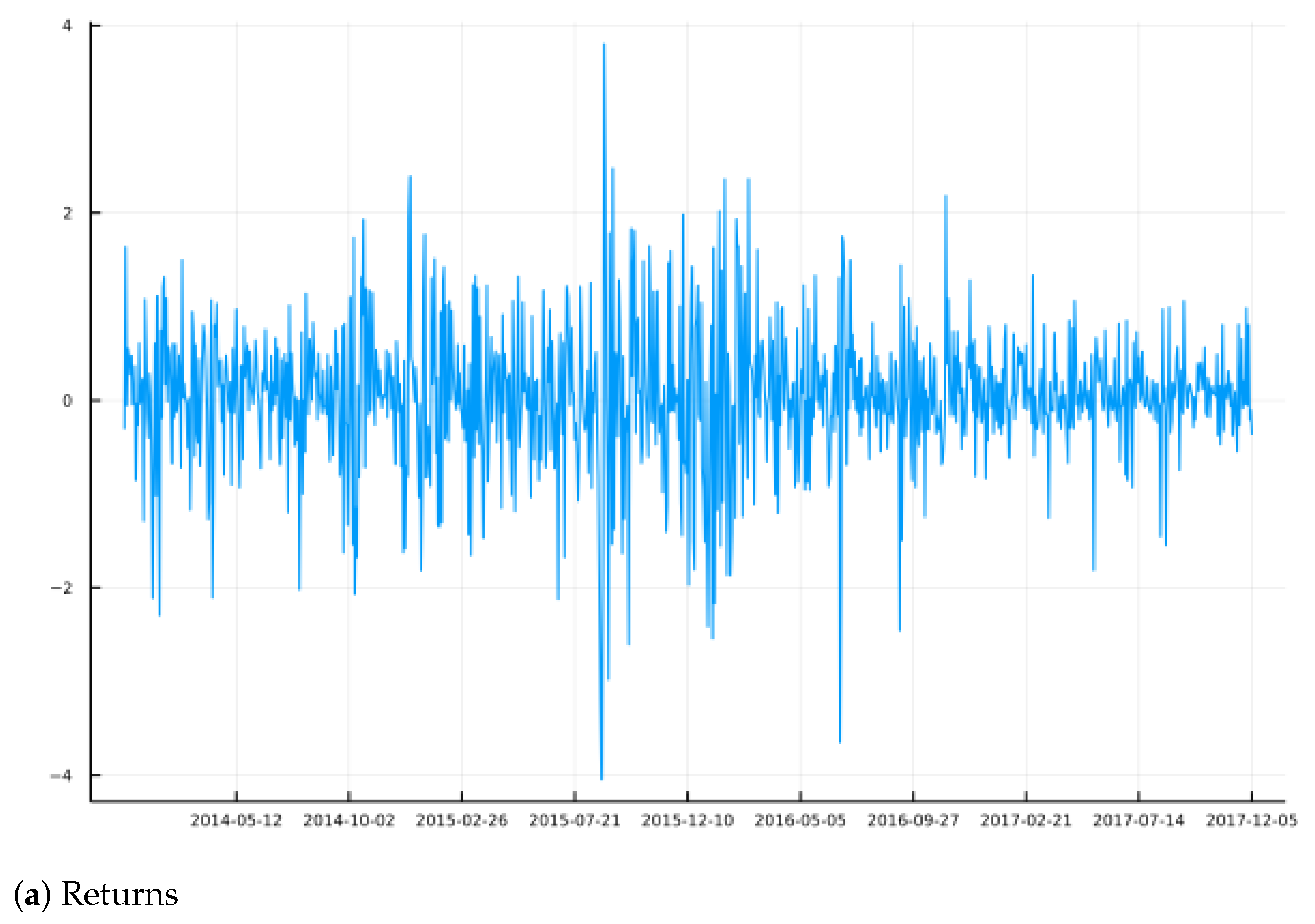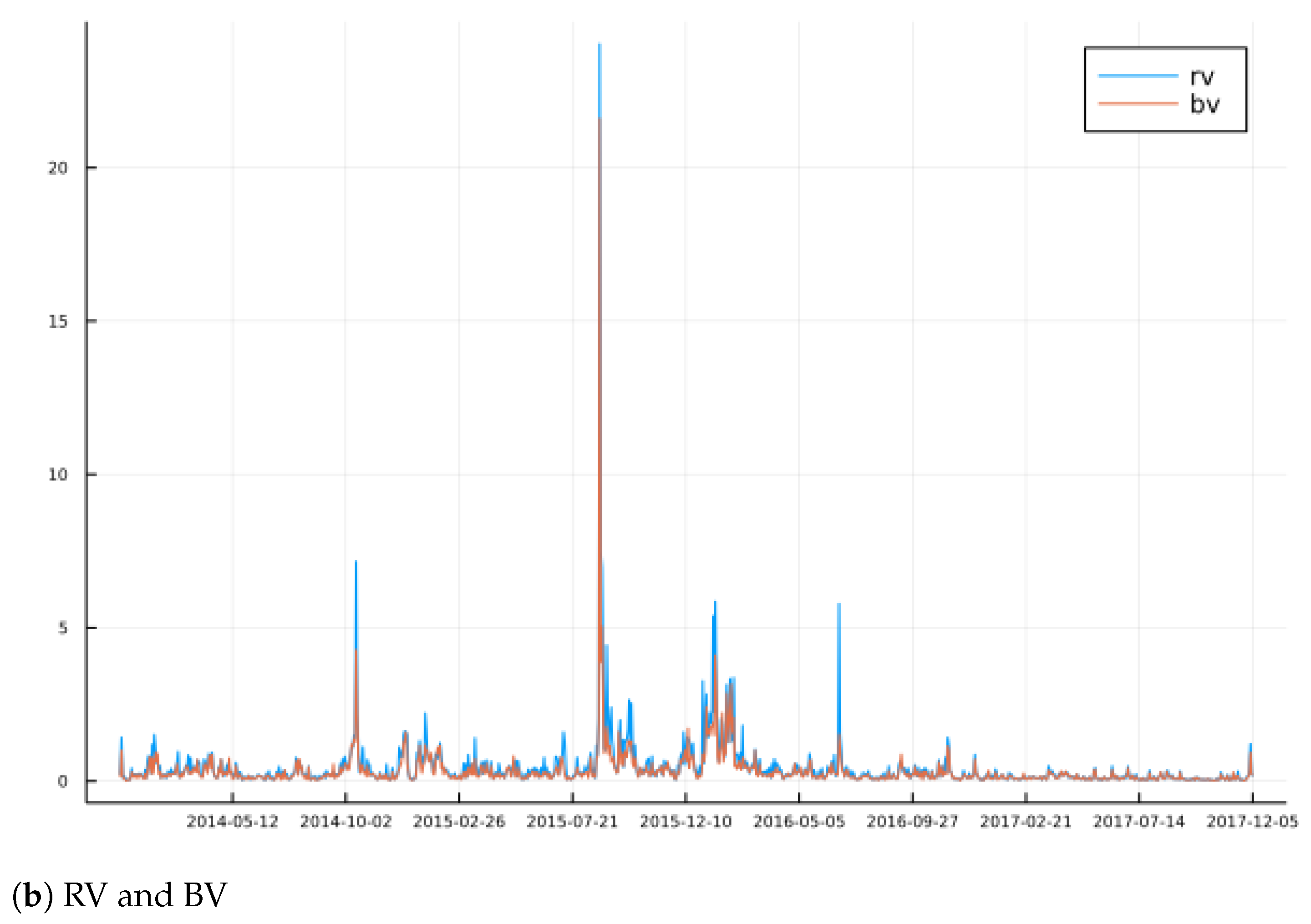Log price, $p_t,$ is simulated using 10-minute tics, and the observed log price adds a $N(0,{\tau }^2)$ measurement error to $p_t$, when $\tau$ is greater than zero. From this model, 1000 daily observations on returns, realized volatility (RV), and bipower variation (BV) are generated. Because log price has been scaled by 100 in the parameterization of the model, returns, computed as the first difference of $p_t$ at the close of trading days, are directly in percentage terms. Both RV and BV are informative about volatility, and, because BV is somewhat robust to jumps, while RV is not, the difference between the two can help to identify the frequency and size of jumps (Barndorff-Nielsen and Shephard 2002). The model is simulated on a continuous 24-hour basis, and returns are computed using the change in daily log closing price, for trading days only. Overnight periods and weekends are simulated, but returns, RV and BV are recorded only at the close of trading days. In summary, the seven parameters are $\theta =(\mu ,\kappa ,\alpha ,\sigma ,\rho ,{\lambda }_0,{\lambda }_1,\tau )$, and simulated data consists of 1000 daily observations on returns, RV and BV. The model studied here is quite similar to that studied in (Creel 2017; Creel and Kristensen 2015), except that the drift process is simplified to be constant, and the jump process is modeled somewhat differently, with constant intensity, and with the magnitude of a jump depending on the current instantaneous volatility. These changes were motivated by the results of the previous papers, and by the better tractability of the present specification.

The raw statistics, $W,$ which are used to train the net and to do estimation, are a combination of coefficients from auxiliary regressions between the three observed variables, summary statistics, and functions of quantiles of the variables. The details of the 25 statistics are found in the file JDlib.jl (this same file also gives details of the priors, which are uniform over fairly broad supports, for all parameters). The neural net was fit using 160,000 draws from the prior to generate the training and testing data. The importance of each of the statistics can be assessed by examining the maximal absolute weights on each of the raw statistics in the first layer of the neural net, as is discussed in Creel (2017). These may be seen in Figure 1. We see that most of the 25 statistics have a non-negligible importance, which means that these statistics are contributing information to the fit of the neural net. The output of the net is of dimension 8, the same as the dimension of the parameters of the model. The net is combining the information of the overidentifying statistics to construct a just-identifying vector of statistics, which is then used to define the moments for MSM-MCMC estimation.

The model was fit, using MSM-MCMC and the CUE criteria, to S&P 500 data13 from 16 December 2013 to 4 December 2017, which is an interval of 1000 trading days, the same as was used to train the neural net. The data may be seen in Figure 2, where we observe typical volatility clusters and some jumps. For example, the Brexit drop of June 2016 is clearly seen, and the more extreme spike in RV versus BV at this point illustrates the fact that jumps can be identified by comparing the two. Over the sample period, this price index climbed from about 1800 to 2600, which is approximately a 44% increase, or approximately 0.04% per trading day.

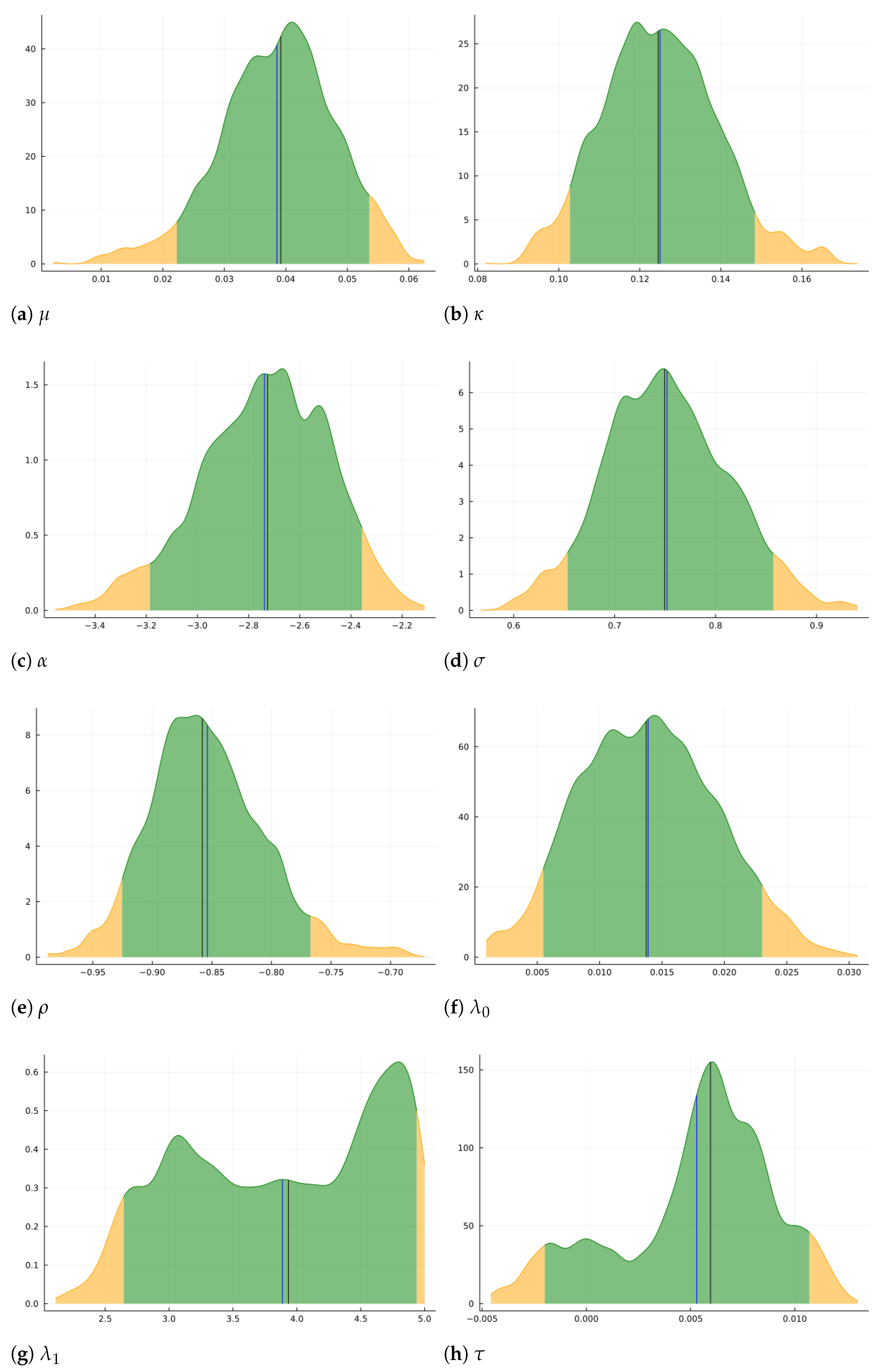
Ten MCMC chains of length 1000 were drawn independently using threads-based parallelization, for a final chain of length 10,000. The estimation results are in Figure 3, which shows nonparametric plots of the marginal posterior density for each parameter, along with posterior means and medians, and 90% confidence intervals defined by the limits of the green areas. All posteriors are considerably more concentrated than are the priors. Drift ($\mu$) is concentrated around a value slightly below 0.04, which is consistent with the average daily returns over the sample period. There is quite a bit of persistence in volatility, as mean reversion, $\kappa$, is estimated to be quite low, concentrated around 0.125. Leverage ($\rho$) is quite strong, concentrated around −0.85. The jump probability per day (${\lambda }_0$) is concentrated around 0.014, and is significantly different from zero. Therefore, jumps are a statistically important feature of the model. When a jump does occur, its magnitude (${\lambda }_1$) is approximately 4 times the current instantaneous standard deviation, but this parameter is not very well identified, as the posterior is quite dispersed. An interesting result is that $\tau$, the standard deviation of measurement error of log price, is concentrated around 0.0055. It is not significantly different from zero at the 0.10 significance level, but it is close to being so. From the Figure, one can see that $H_o:\tau <0$ would be very close to being rejected at the 10% significance level. The parameterization of the model is such that there is no measurement error when $\tau \le 0$. Thus, it appears that it is a safer option to allow for measurement error in the model, as the evidence suggests that it is very likely present, and its omission could bias the estimates of the other parameters.

7. Conclusions

This paper has shown, through Monte Carlo experimentation, that confidence intervals based upon quantiles of a tuned MCMC chain may have coverage which is far from the nominal level, even for simple models with few parameters. The results on poor reliability of inferences when using overidentified GMM estimators, which were referenced in the Introduction, carry over to a Bayesian version of overidentified MSM, implemented using the Chernozhukov and Hong (2003) methodology, for the models considered in this paper. The paper proposes to use neural networks to reduce the dimension of an initial set of moments to the minimum number of moments needed to maintain identification, following Creel (2017). When estimation and inference using the MSM-MCMC methodology is based on neural moments, which are exactly identifying, confidence intervals have statistically correct coverage in all cases studied by Monte Carlo, when the CUE version of MSM is used. Thus, there seems to be no generic problems with the MSM-MCMC methodology for the purpose of inference. A potential problem has to do with the choice of moments upon which MSM is based. Too much over-identification results in poor inferences, for the models studied. The use of neural moments solves this problem, by reducing the number of moments, without losing the information that they contain. The fact that RMSE does not rise when one moves from raw to neural moments illustrates that the neural moments do not lose the information that is contained in the larger set. The methods have been illustrated empirically by the estimation of a jump-diffusion model for S&P 500 data. An interesting result of the empirical work is that measurement error in log prices is likely to be present.

It is to be noted that the step of filtering moments though a neural net is very easy and quick to perform using modern deep learning software environments. The software archive that accompanies this paper provides a function for automatic training, requiring no human intervention. It only requires functions that provide simulated moments computed using data drawn from the model at parameter values drawn from the prior. Filtering moments through a neural net gives an informative, minimal dimension statistic as the output. This provides a convenient and automatic alternative to moment selection procedures. Uninformative moments are essentially removed, and correlated moments are combined.

This paper has examined how inference using the MSM-MCMC estimator may be improved when neural moments are used instead of a vector of overidentifying moments. It seems likely that other inference methods which are used with simulation-based estimators, such as Hamiltonian Monte Carlo and sequential Monte Carlo, among others, may be made more reliable if neural moments are used, as dimension reduction while maintaining relevant information is likely to be generally beneficial.