Abstract
(Hendry 1980, p. 403) The three golden rules of econometrics are “test, test, and test”. The current paper applies that approach to model the forecasts of the Federal Open Market Committee over 1992–2019 and to forecast those forecasts themselves. Monetary policy is forward-looking, and as part of the FOMC’s effort toward transparency, the FOMC publishes its (forward-looking) economic projections. The overall views on the economy of the FOMC participants–as characterized by the median of their projections for inflation, unemployment, and the Fed’s policy rate–are themselves predictable by information publicly available at the time of the FOMC’s meeting. Their projections also communicate systematic behavior on the part of the FOMC’s participants.
1. Introduction
A central tenet of modern macroeconomics is that the effectiveness of monetary policy rests on its policy being understood by the public. To this end, U.S. monetary authorities have been releasing since 2007 their Summary of Economic Projections (SEP) to enhance the public’s understanding of their policies:
The Federal Open Market Committee (FOMC) announced on Wednesday that, as part of its ongoing commitment to improve the accountability and public understanding of monetary policy making, it will increase the frequency and expand the content of the economic projections that are made by Federal Reserve Board members and Reserve Bank presidents and released to the public.(FOMC Press Release 14 November 2007)
Further, these projections are tied to the participants’ views of appropriate monetary policy:
Appropriate monetary policy is defined as the future policy most likely to foster outcomes for economic activity and inflation that best satisfy the participant’s interpretation of the Federal Reserve’s dual objectives of maximum employment and price stability.(FOMC Minutes, 31 October 2007, p. 9)
Reference (Faust 2016, p. 17), however, notes that:
Faust’s position raises several questions. Specifically, does the absence of hints imply the absence of any information? Indeed, is understanding monetary policy, as sought by the SEP, limited to discovering such hints? If not, what empirical alternatives might be available? Addressing these questions is the goal of this paper.The SEP, in my view, deserves a special place in the annals of obfuscation in the service of transparency. The SEP is purely a depiction of the policymakers’ different views on the outlook and appropriate policy, with no hints about how any differences may be resolved.
Our analysis of the FOMC’s projections focuses on release dates, delays in release, the forecast process, and forecast assessment. To be sure, the paper’s focus is not on the dispersion of the projections, nor on the projections of a given individual per se, nor on how the voting gives rise to the interest rate decisions. Section 2 examines the FOMC’s idiosyncratic release protocol. In essence, the FOMC releases summaries of economic projections in three phases: a summary of the forecasts immediately after the FOMC meeting, additional details of that meeting five years later, and remaining details ten years later. Section 2 also analyzes the information loss from such delays. Using publicly available information, Section 3 models the median participant’s forecasts for inflation, unemployment, and the appropriate interest rate.1 The paper focuses on these variables for several reasons. First, the Press Releases of FOMC decisions focus on them. Second, policy documents, such as the Bluebook (released with a delay), show that the alternatives over which FOMC members vote focus on unemployment and inflation. Third, data for GDP growth are revised with a greater frequency and extent than measures of inflation and unemployment. Section 3 considers several formulations, the results of which are closely aligned with the familiar Taylor rule. The paper’s framework is consistent with the FOMC record. These models could have been rejected by the data. Our framework also provides a basis for mapping FOMC projections into FOMC interest rate decisions. Section 4 assesses those results, focusing on predictive accuracy and responses to forecast revisions.2 Section 5 concludes.
2. FOMC Forecasts
This section documents the structure of the FOMC and the assembly of the data for the medians of its projections from 1992 to 2019. All publications by the FOMC are available on the Federal Reserve Board’s website (www.federalreserve.gov, accessed on 8 September 2021).
2.1. Participants
The FOMC consists of 19 participants: 12 Presidents from the Federal Reserve Banks and 7 Governors from the Board of Governors of the Federal Reserve System; only 12 participants vote in a given FOMC meeting. The voting participants are the seven governors of the Federal Reserve Board, the President of the New York Federal Reserve Bank, and four other presidents on a rotating basis. The FOMC is scheduled to meet eights times per year and releases its projections after scheduled meetings. The details of such releases have changed in terms of frequency, horizon, and content; the FOMC also meets occasionally outside its schedule via conference calls.
2.2. Frequency and Horizon
From 1992 to 2007, projections were released twice per year (February and July) in the Monetary Policy Report (MPR). February meetings reported projections for the current year; July meetings reported projections for the current year and one year ahead (Table 1).

Table 1.
MPR target year (1995–1998).
Since 2007, projections are released four times per year in the Summary of Economic Projections (SEP). Participants forecast the current year and the next two years ahead. During the last two meetings of each year, the participants extend their projections by one year (Table 2). The SEP also includes a long-run horizon defined as “⋯each participant’s assessment of the rate to which each variable would be expected to converge under appropriate monetary policy and in the absence of further shocks to the economy”.
Table 2.
SEP target year (2010–2015).
Table 3 documents the increase in the information associated with the immediate release of the Summary of Economic Projections. Specifically, participants’ projections for the appropriate interest rate have been included since 2012, and the median of the forecast distributions for GDP, inflation, unemployment, and the appropriate interest rate have been reported since 2015. As the SEP describes, “[t]he range for a variable in a given year includes all participants’ projections, from lowest to highest, for that variable in that year”, and “[t]he central tendency excludes the three highest and three lowest projections for each variable in each year”. For the purposes of this paper, the midpoint of the forecast range is the average of the lowest and the highest values of the range.
Table 3.
Evolution of the Survey of Economic Forecasts.
2.3. Content
Information about the FOMC forecasts are made public in three steps:
- Immediate. Immediately after the relevant meeting, the FOMC releases information that includes participants’ forecast range and central tendency for GDP growth, inflation, and unemployment;
- Five-year delay. With an approximate five-year delay, the FOMC releases participants’ individual projections (without attribution) and the Tealbook forecasts from the staff of the Federal Reserve Board;
- Ten-year delay. With an approximate ten-year delay, the FOMC releases the participants’ individual projections with attribution, i.e., naming which participant made which forecast.
Table 4 summarizes the data availability from FOMC releases and how this availability has changed over time.
Table 4.
Data availability of FOMC forecasts.
2.4. Appropriate Federal Funds Rate
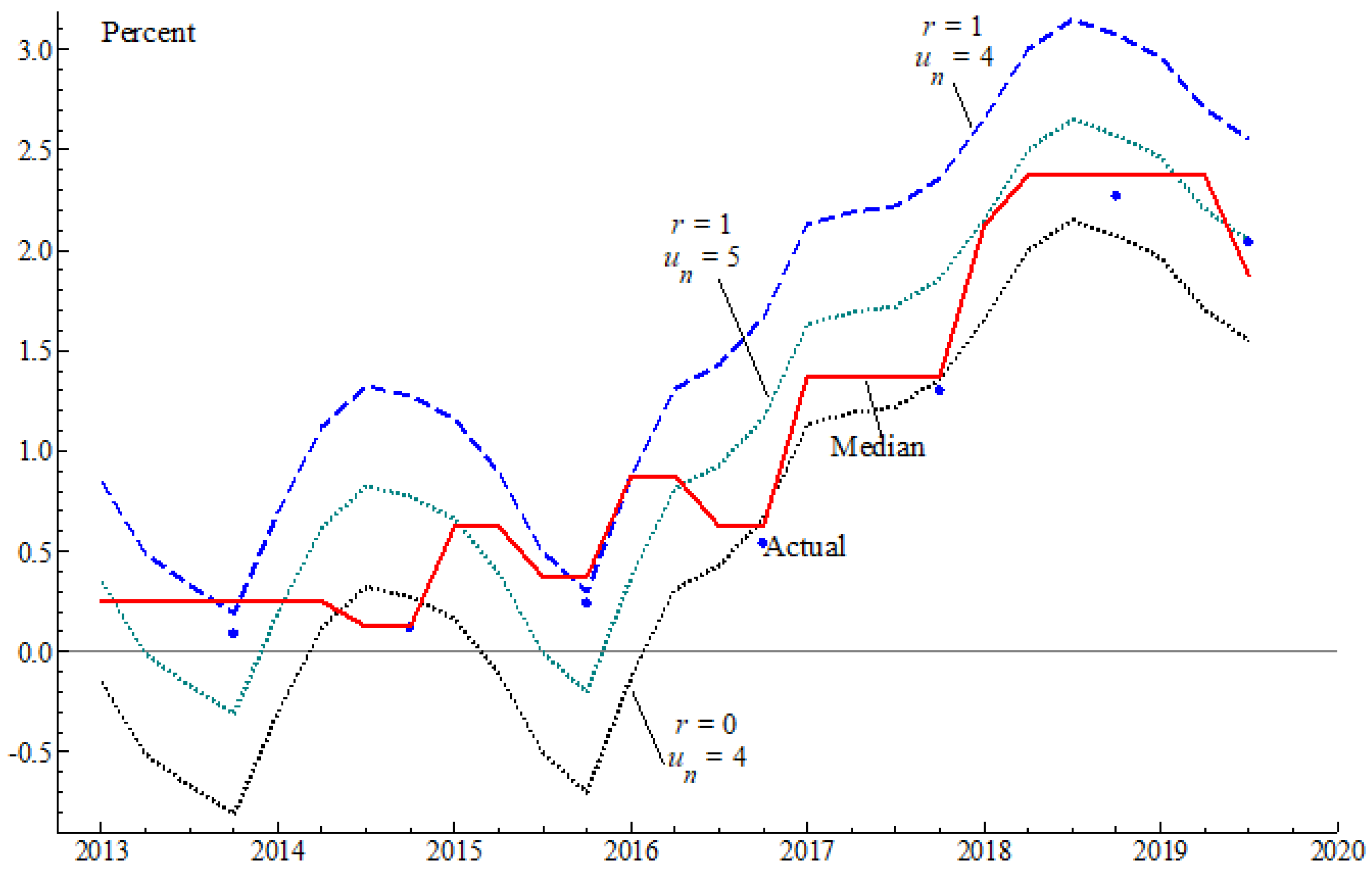
Figure 1 shows participants’ reported forecasts, in the current year, of the appropriate federal funds rate at the end of the current year. Note that the SEP reports participants’ forecasts, rounded to the nearest 1/8 percentage point. As a result, several participants may share the same reported value of the appropriate interest rate, even though their underlying views might differ slightly.
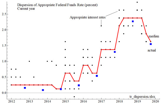
Figure 1.
Appropriate federal funds rates for the end of the current year. Participants’ forecasts are shown as black circles; the median of the forecast distributions are shown in red; the actual values of the federal funds rate in Q4 of each year are shown as blue squares.
Figure 1 shows that, despite the dispersion of participants’ views on the appropriate rate, the median of the distribution from each meeting is close to the actual rate. Thus, if there is a reliable empirical model for this median, then the SEP would be informative, so it would diminish the force of Faust’s critique.
2.5. Inflation and Unemployment Forecasts
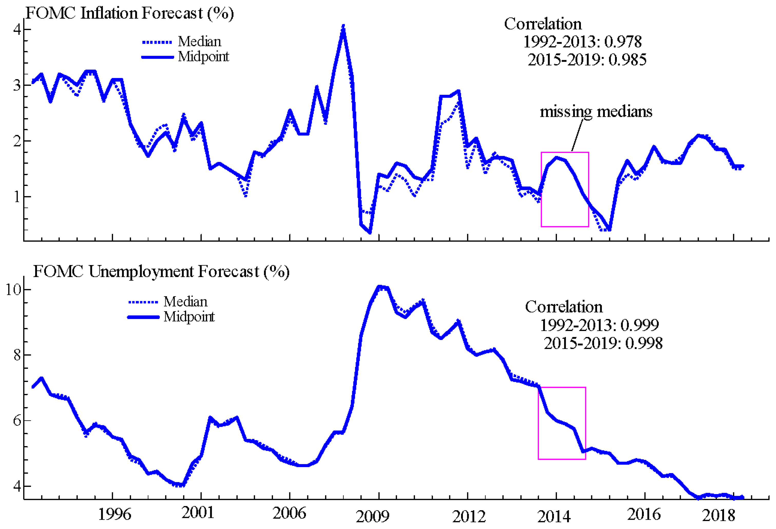
Data for the median of the distribution of participants’ inflation and unemployment forecasts involve combining information from the immediate and delayed releases. Data for 1992–2012 are computed using the participants’ forecasts from delayed releases (Table 4). Data for the median of forecasts from 2015:Q3 to 2019:Q3 are available from the immediate releases (Table 4). Data from 2013:Q1 to 2015:Q2, however, are not currently available from existing releases. Thus, the paper examines whether the midpoints of the forecasts’ range for 2013:Q1 to 2015:Q2 (always available) offer a suitable substitute for the missing values of the median. Figure 2 reveals that movements in the median and the midpoint from FOMC forecasts are closely associated with each other.
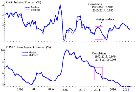
Figure 2.
Median and midpoint of FOMC forecast distributions.
Further, Table 5 shows that differences between the medians and the midpoints are numerically very small.
Table 5.
Medians and midpoints of FOMC forecast distributions.
Thus, the paper treats the midpoints of the forecast distributions over 2013:Q1–2015:Q2 as equivalent to the respective medians. This assumption will be relaxed once the FOMC releases further details for this period.
2.6. Loss of Information from Delayed Releases
This section assesses the potential loss of information from delaying the release of the Federal Reserve Board’s staff forecasts, as reported in the Greenbook. The Greenbook, officially entitled “Current Economic and Financial Conditions”, provides in-depth analysis of the U.S. and international economy. It is produced by the staff at the Board of Governors and has been distributed to FOMC meeting attendees approximately a week before the meeting. After 2010, the Greenbook was restructured and became the Tealbook.
The equations used to determine the loss of information are:
where and are vectors of unknown coefficients, and are the medians of the distributions of the FOMC inflation and unemployment forecasts issued in period p for target year and is the vector of exogenous variables in period Table 6 below lists the variables and their definitions.
Table 6.
List of mnemonics and definitions.
These equations examine whether the current period’s median, conditional on the prior meeting’s midpoint, is explainable by the Greenbook forecast and by information publicly available prior to the current meeting. Allowance for Chair-specific effects may capture declines in the neutral rate (Bernanke 2016; Powell 2018) and recognizes that FOMC Chairs’ influence the appropriate rate. If the coefficients associated with the Greenbook forecasts are significant, then the delay in releasing the Greenbook forecasts entails a loss of information provided to the public about the SEP when initially released.
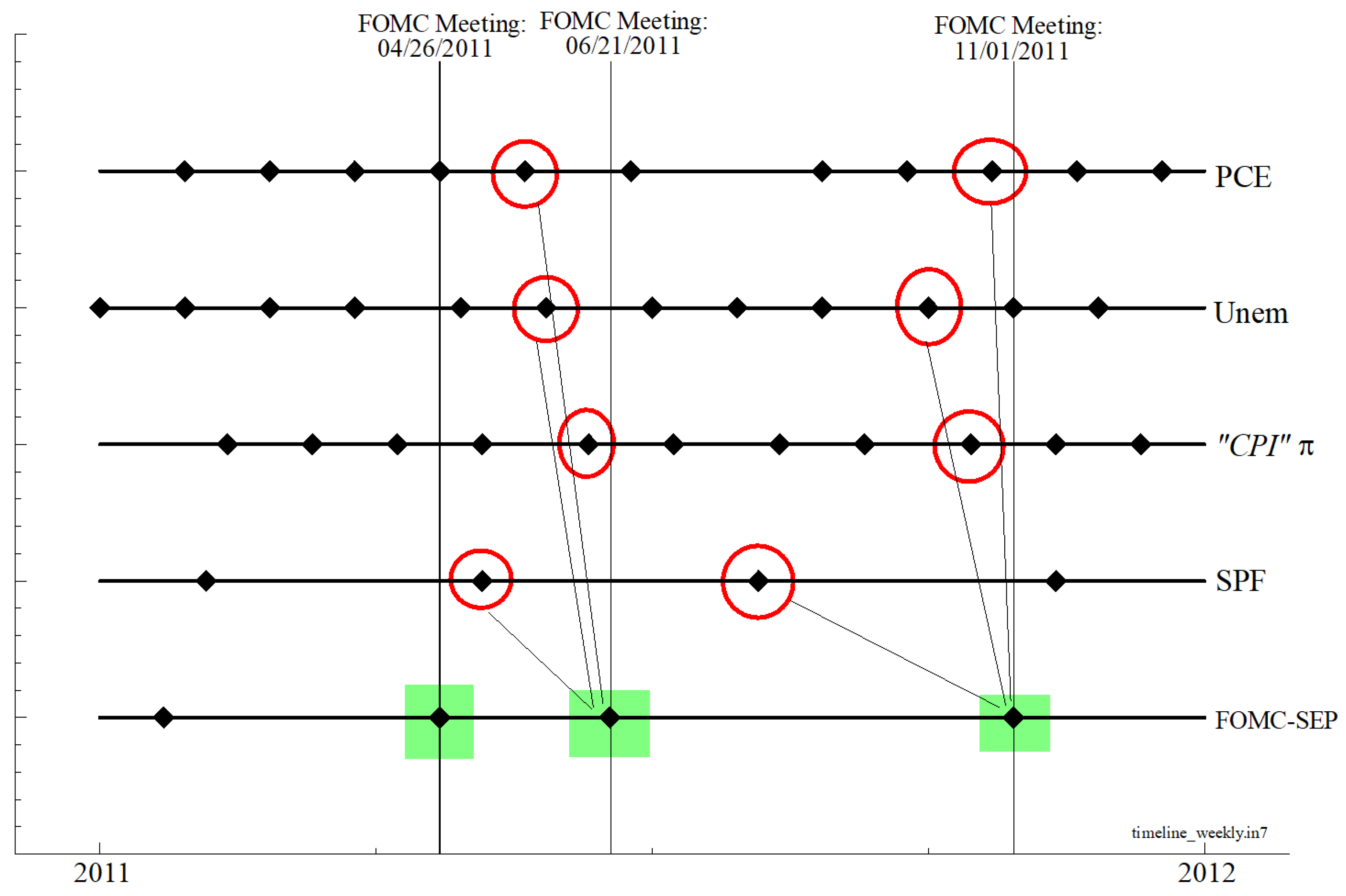
Figure 3 shows the timeline of the publicly available data for the explanatory variables immediately prior to the FOMC meeting. Note that the calendar of FOMC meetings is set independently of the calendar of public data releases, which, in turn, are not aligned over time or with each other. For example, the Survey of Professional Forecasters (SPF) is released on a quarterly basis (in February, May, August, and November), whereas the Bureau of Labor Statistics (BLS) releases its data on a monthly basis. Hence, the lapse of time between the availability of public data and the FOMC meeting is not fixed. For estimation purposes, the regression uses information that is publicly available immediately prior to the FOMC meeting. The measure of inflation targeted by the FOMC changes over time: the CPI from January 1992 to July 1999; the PCE from January 2000 and January 2004; the Core PCE starting in July 2004.
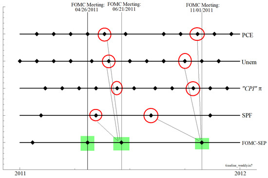
Figure 3.
Timeline of releases of public data. Each horizontal line shows the release dates for the selected variable. The red circles denote the date of the variable used; the green square corresponds to the Greenbook.
The estimation sample is from January 1992 to March 2015 owing to the delayed release of the Greenbook. Parameter estimation relies on a general-to-specific estimation strategy, which is implemented with autometrics as developed by Doornik and Hendry (2018). Their approach avoids the statistical pitfalls associated with the joint nature of model specification and parameter estimation. Selecting a critical value for deleting a variable involves a tradeoff between excluding relevant variables and including irrelevant variables. The current paper uses a strategy with a target size of one percent, where the target size is defined as “the proportion of irrelevant variables that survives the [simplification] process” (Doornik 2009, p. 100).
For the median inflation forecast, the results from the general formulation reject the joint exclusion of the Greenbook forecasts (Table 7). For the final model selected, the two explanatory variables are the lagged midpoint and the lagged inflation forecast from the Greenbook. One cannot reject the hypothesis of white noise residuals.
Table 7.
Models of FOMC forecasts.
For the median unemployment forecast, the results for the general formulation reject the joint exclusion of the Greenbook forecasts (Table 7). One cannot reject the hypothesis that the coefficient for the midpoint of the unemployment forecast range is equal to one. For the final model, the relevant variables are the lagged midpoint and the lagged Greenbook forecasts.
Taken together, the results reveal two findings of interest. First, the medians of the FOMC forecasts for inflation and unemployment are partially explained by public data available prior to the FOMC meeting. Second, the Greenbook forecasts are relevant for explaining the median of the FOMC’s forecasts. Thus, delaying the release of the Greenbook forecasts impairs the public’s ability to predict the FOMC’s predictions. Even if released on a more timely basis, the Greenbook still could be valuable as “private” information to the FOMC. It could be reflected in the midpoint, similar to the findings in (Bespalova 2018; Ericsson 2016; Stekler and Symington 2016, chp. 3) for FOMC minutes and the Greenbook.
3. Models of the Projected Appropriate Interest Rate
This section develops empirical models to explain the medians of the distribution of the FOMC’s forecasts of the appropriate interest rate.
3.1. Single-Equation Models
Critics of the SEP argue that the FOMC should make its reaction function available to the public. For example, Faust states that “...As noted above, the most important function to convey regards the reaction function of the policymakers” (Faust 2016, p. 18). Further, (Bernanke 2016, p. 7) states that,
Wouldn’t it be easier if the FOMC just provided its reaction function, together with collective projections of key macroeconomic variables? In principle, yes; and in fact, in the course of expanding the SEP, the FOMC under my chairmanship experimented with developing a consensus committee forecast, together with alternative scenarios, that could be released to the public.
In the absence of an official reaction function, the paper uses the Taylor rule, with assumed coefficients, to examine whether FOMC decisions are consistent with their own projections for inflation and unemployment. Specifically, the Taylor rule used here is:
where is the median of the FOMC projections for the appropriate federal funds rate issued in period p for target year t.3 Figure 4 shows the values for using two values for the target real rate r () and two values for the natural rate of unemployment () (see Bernanke 2016; Powell 2018).

Figure 4.
Taylor rule calculations for the appropriate federal funds rate.
Figure 4 reveals that reliance on Equation (3) injects an ambiguity in the stance of monetary policy. If and then monetary policy has been expansionary since 2013, whereas if and the stance has been generally contractionary. This ambiguity arises despite the calculations using the FOMC’s own measure of inflation and unemployment forecasts.
The calculations in Figure 4 rest on the specification of the Taylor rule and the values of its coefficients. One approach to relax the assumption of known coefficients involves estimating the parameters of:
where . Parameter estimation relies on the general-to-specific estimation strategy using observations from 2012–2019 (32 observations). Note that Equation (4) does not identify two parameters, namely r and
The results are in Table 8. From the final model obtained, an increase of one percentage point in the median of the forecast unemployment rate lowers the current period median federal funds rate by 32 basis points. Furthermore, the coefficient for Yellen’s tenure is significant.
Table 8.
Estimation results for Equation (4).
Because and are released simultaneously, reliance on this equation only helps to detect ex post inconsistencies between predictions and decisions. Thus, it is fair to ask whether relying on data available prior to the meeting helps predict ahead of the meeting. The formulation used to examine this question is:
where The results reveal two features of interest (Table 9).
Table 9.
Estimation results for Equation (5).
First, the SPF forecasts are the only economic indicators relevant for predicting in the final model. Second, the coefficient for Yellen’s tenure is significant.
The results from Table 8 and Table 9, when considered as a whole, reveal empirically reliable and economically meaningful models explaining the median of the projected appropriate rate. Further, the estimates are quite close (though not identical) to the ones assumed in the Taylor rule. These findings have shortcomings. First, the SEP’s projections for these variables are, arguably, jointly determined. In other words, there might be value in jointly forecasting the FOMC forecasts for inflation, unemployment, and the appropriate interest rate. Second, each participant forecasts at multiple horizons. Those forecasts may be jointly determined and so may be affected by periodic extensions of the horizon by the FOMC.
3.2. Multi-Equation Models
This section develops multi-equation models to explain the median of the FOMC current and one-year-ahead projections for inflation, unemployment, and the appropriate rate.
3.3. Data
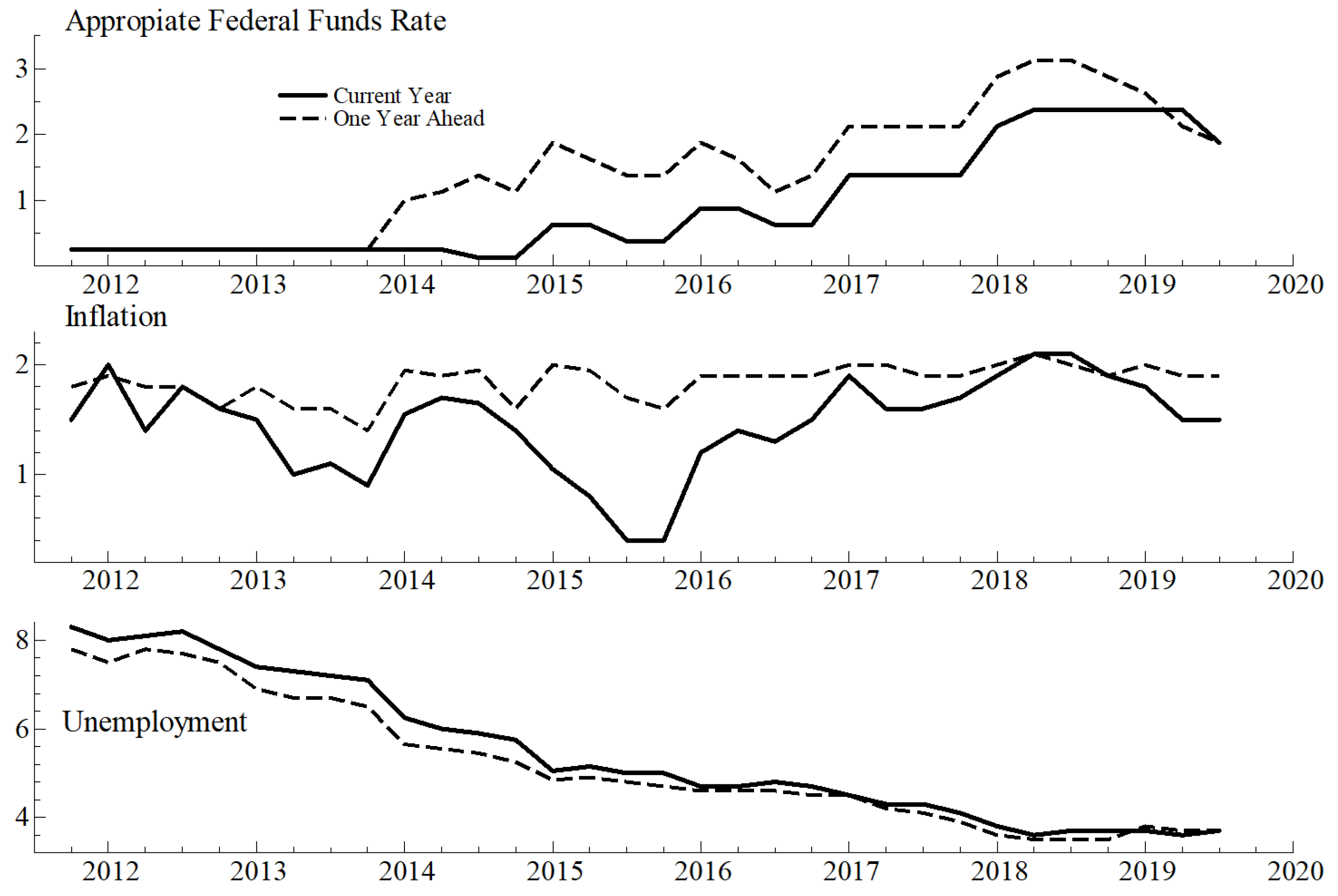
Figure 5 shows the evolution of the medians of the forecasts for the six variables of interest:
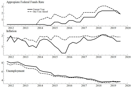
Figure 5.
Median of FOMC forecasts: current and one-year-ahead.
The data show that differences between current and one-year-ahead projections have been generally one-sided. For example, the projected rate one year ahead has been, until recently, equal to the current-year rate plus a fairly constant differential. For inflation, the one-year-ahead projections oscillate around two percent, even though the current-year projection is considerably lower. For unemployment, the projections reveal sustained optimism: the one-year-ahead forecast is lower than the current-year one.
3.4. Empirical Formulations
We considered two formulations of a first-order VAR augmented with exogenous variables for which data are publicly available. The first formulation is an unrestricted VAR:
where:
- is the inflation projection issued in period p for target year ;
- is the unemployment projection issued in period p for target year ;
- is the federal funds rate projection issued in period p for target year ;
- ;
- This model has 78 coefficients.
The second formulation restricts Equation (6) to a recursive structure in which projections for the current-year determine the one-year-ahead projections, but not the other way around. The bloc for the current-year projections is:
The bloc for the one-year ahead projections is:
where The variance–covariance matrix is symmetric and positive definite, but otherwise unconstrained. Note that the equation for uses the endogenously determined FOMC projections for inflation and unemployment.
Equation (7) has 39 coefficients, resulting from imposing 39 restrictions on Equation (6). There are several motivations for these restrictions:
- B and rule out cross-persistence effects. Specifically, affects , but not ;
- C shows that the use of publicly available data is targeted. For example, and affect , but not
The restricted FIML coefficient estimates are shown in the Appendix B. Relative to Equation (6), a log-likelihood ratio test rejects the second formulation (Equation (7)), which underscores the tentative nature of this work.
3.5. Estimation Results
The estimation results reveal several features of interest:
- (1)
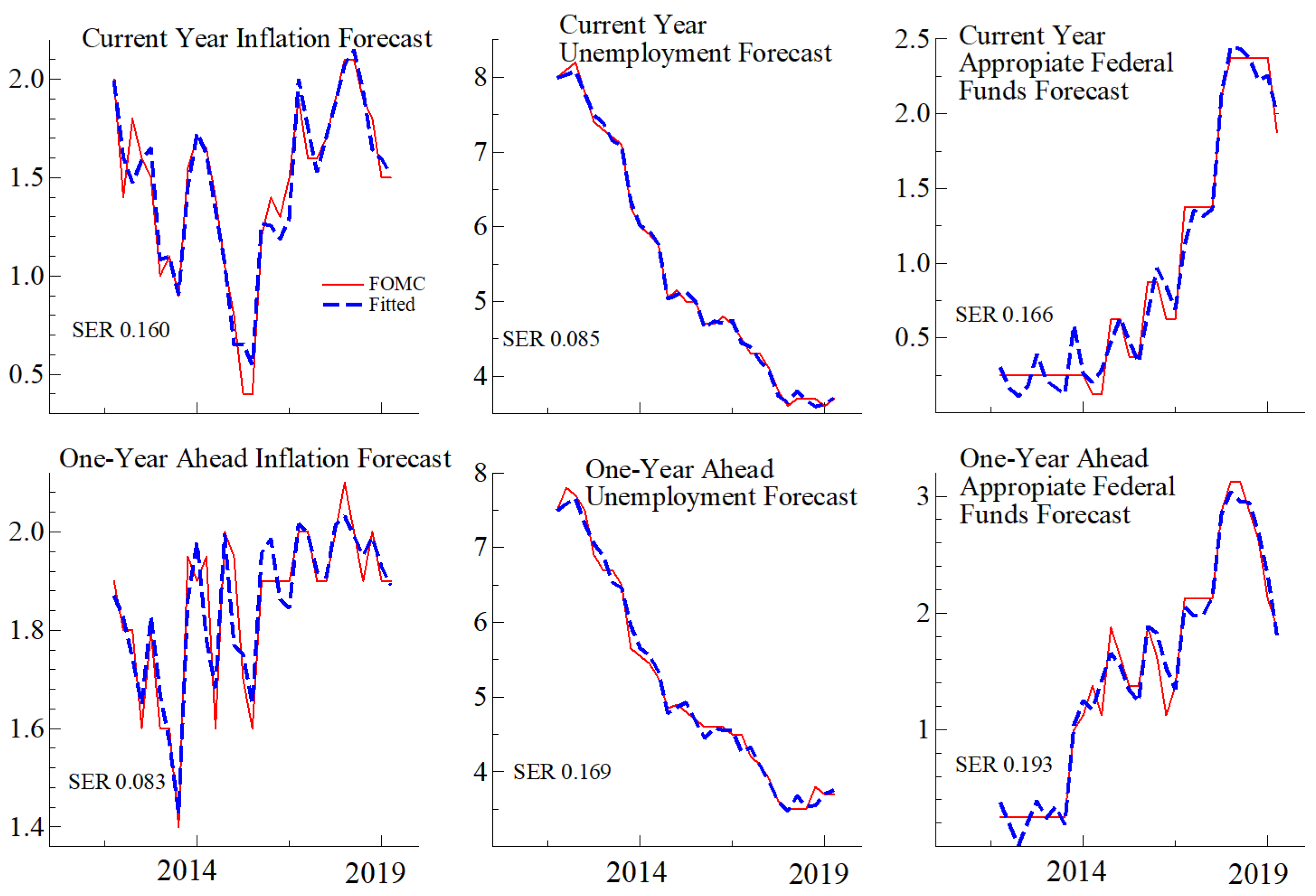
- Figure 6 and Figure 7 show that the predictive accuracy of the unrestricted model (Equation (6)) is greater than that of the restricted model (Equation (7));
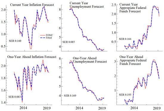 Figure 6. Model fit for the unrestricted VAR Equation (6).
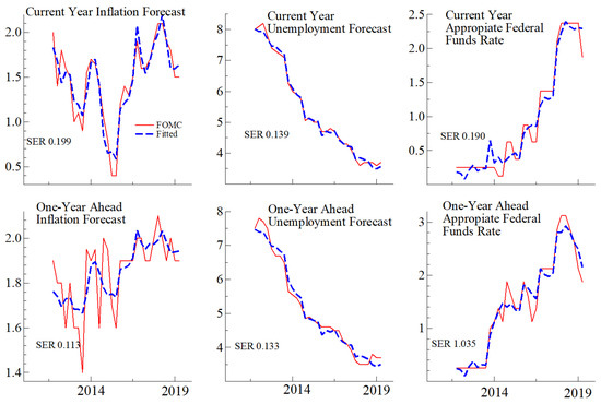 Figure 7. Model fit for the restricted VAR Equation (7).
 - (2)
- Table 10 reports the test statistics for the hypothesis of serial independence, homoscedasticity, and normality applied to the individual equation’s residuals and to the associated vector of residuals. The results indicate mixed support for these properties;
Table 10. Test of residual properties .
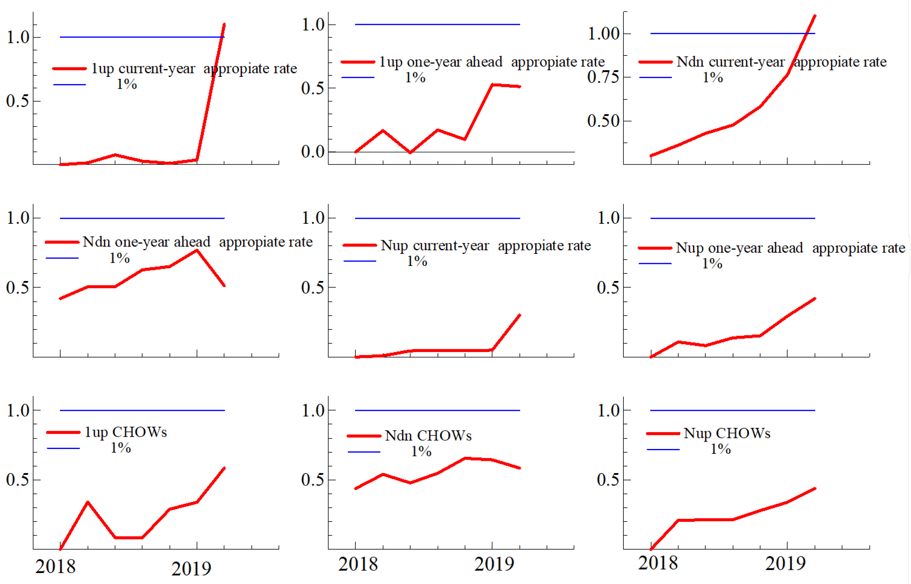
- (3)
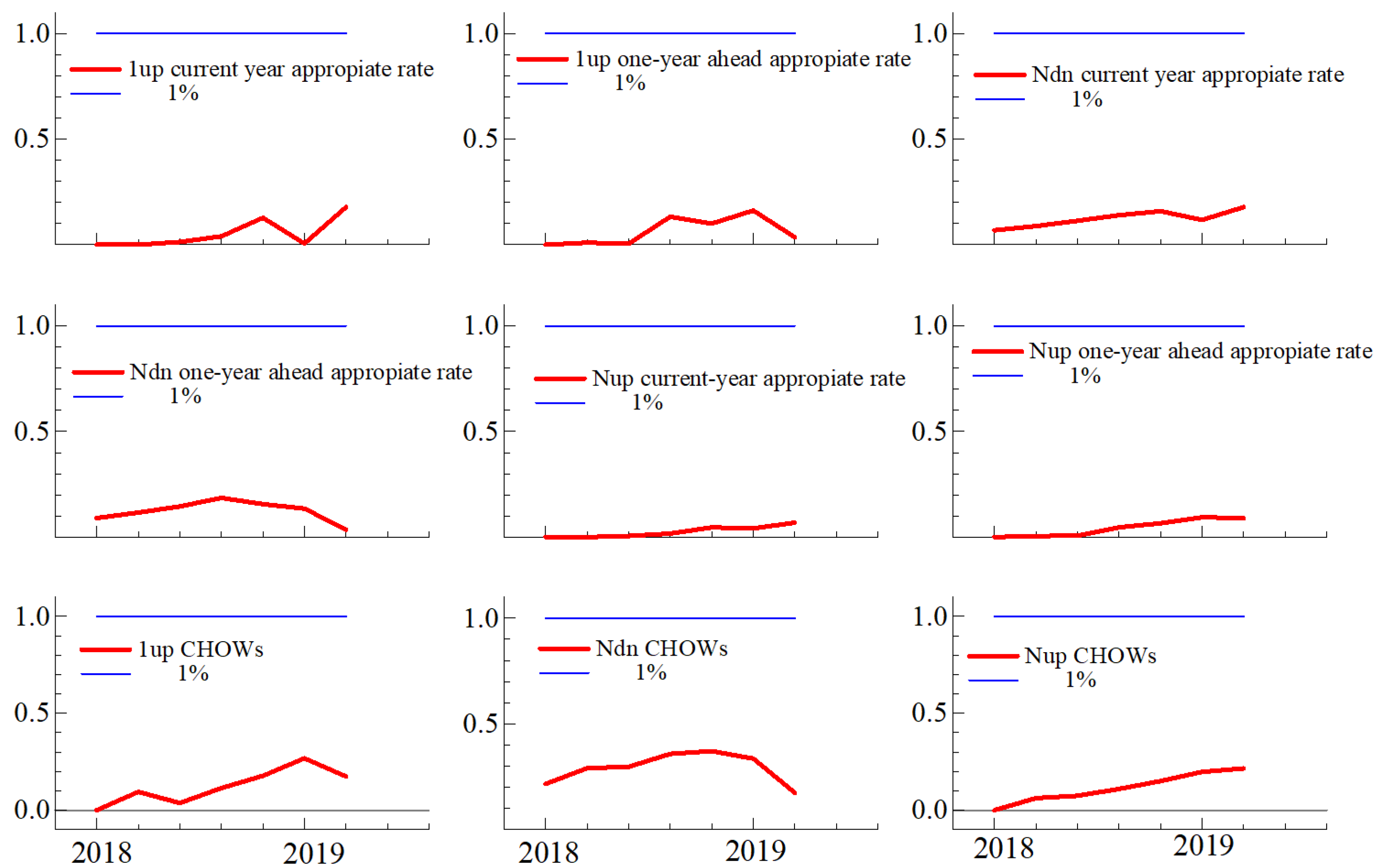
- Figure 8 and Figure 9 report three sequences of recursive Chow test statistics: one-step-ahead (1up); N-periods-ahead, where N decreases as the estimation sample increases (N N-periods-ahead where N increases as the estimation sample increases (N. The focus is on and the system as a whole (“CHOWs”). The test statistics are well below the one-percent critical rejection value, except for in 2019 using the restricted model.
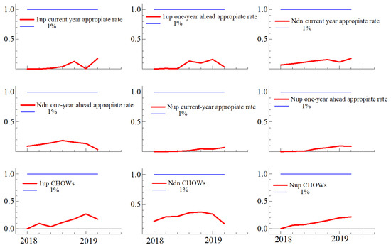 Figure 8. Recursive Chow tests for the unrestricted VAR (Equation (6)).
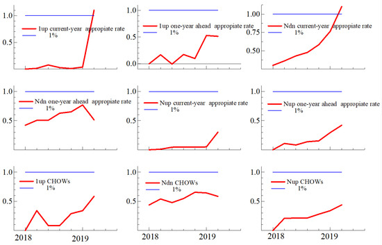 Figure 9. Recursive Chow tests for the restricted VAR (Equation (7)).
3.6. Model Fit
3.7. Congruency: Residuals
Table 10 below reports the results of testing three properties of the residuals (Serial Independence, Homoskedasticity, and Normality) for both models
3.8. Congruency: Recursive Chow Tests
4. Assessing the Models’ Usefulness
This section compares the models’ forecasts of the FOMC forecasts to the FOMC forecasts as such and examines the models’ responses to unanticipated forecast revisions to inflation and unemployment.
4.1. Predictive Accuracy
To assess the out-of-sample predictive accuracy, the models’ parameters were re-estimated excluding the last two observations and then used to generate one-step-ahead out-of-sample forecasts for the SEPs from June and September 2019. The results revealed several features (Table 11).
Table 11.
One-step-ahead forecasts for the median of the FOMC projections. Alternative models (entries in parentheses are the forecast’s standard error).
First, the unrestricted VAR generally exhibits greater predictive accuracy than the restricted VAR and has small and statistically insignificant prediction errors for . Second, prediction errors for (and for for September 2019) are large and statistically significant for the restricted model.
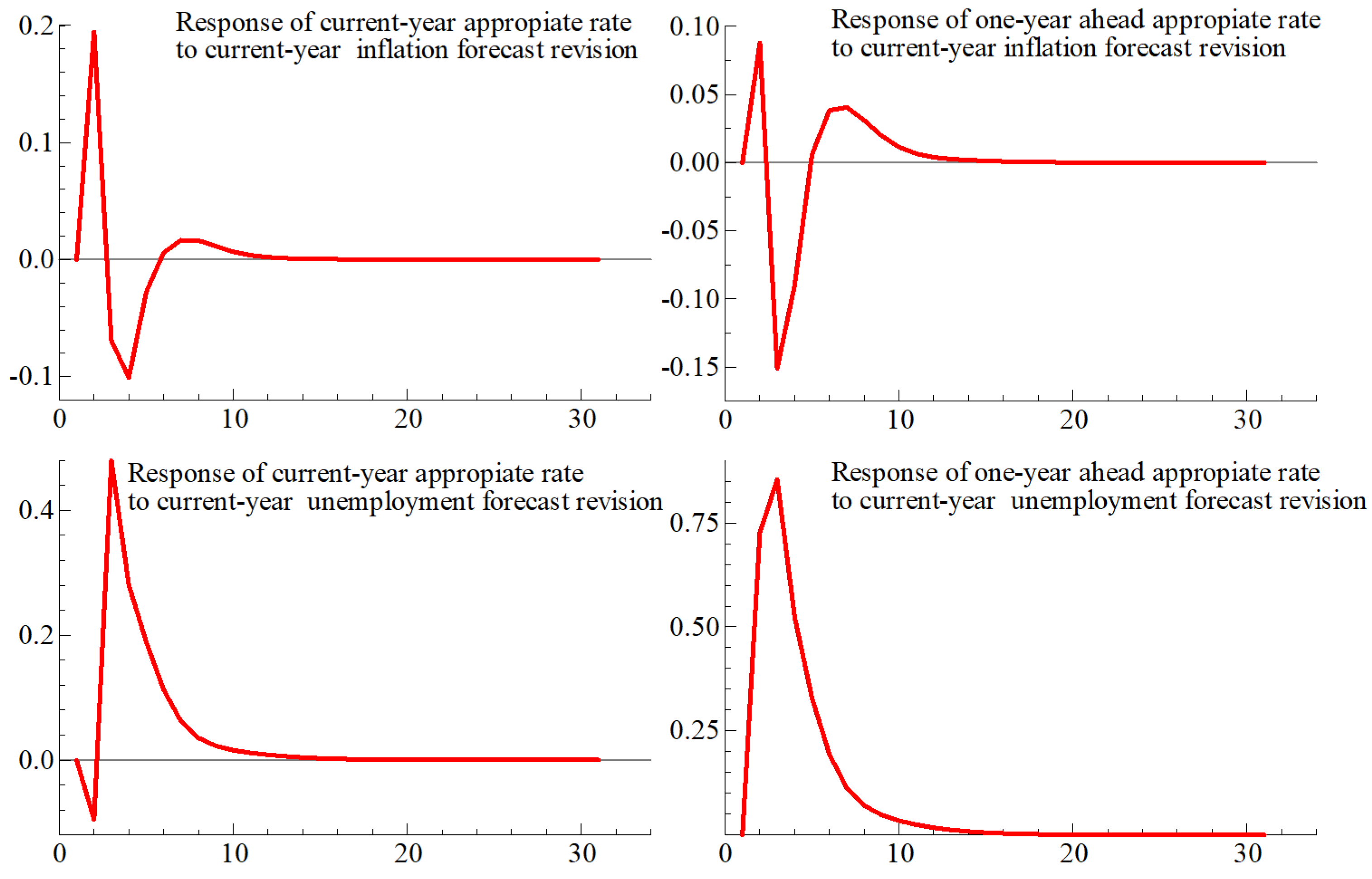
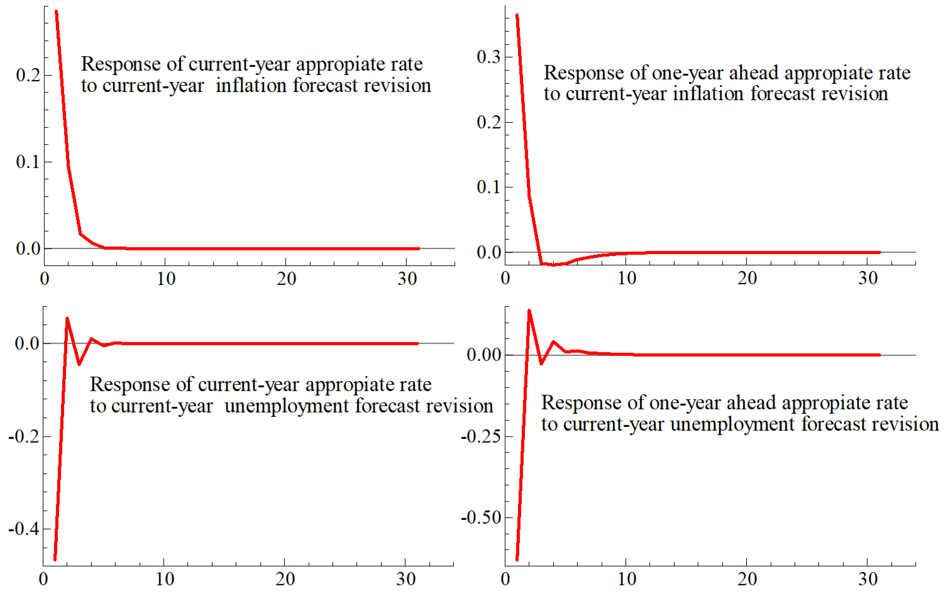
4.2. Forecast Revisions
A central feature of the FOMC forecasting protocol is the opportunity for participants to revise their forecasts for a given target date. Indeed, FOMC participants may issue as many as 12 forecasts for each target date (Table 3). Thus, and following Bernanke’s suggestion of reporting alternative scenarios (see page 8), Figure 10 and Figure 11 report impulse responses to revisions in inflation and unemployment forecasts. These responses are consistent with macroeconomic theory if and :
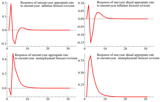
Figure 10.
Effect of forecast revisions: unrestricted VAR Equation (6).
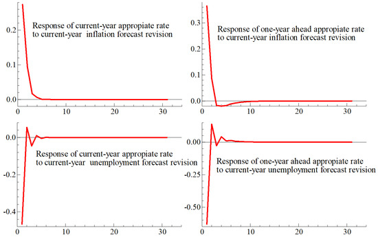
Figure 11.
Effect of forecast revisions: restricted VAR Equation (7).
- Figure 11 shows that a transitory, one percentage point upward revision in ( see Equations (6) and (7)) raises by 40 basis points and by 80 basis points in the unrestricted VAR. These increases contradict existing macroeconomic theory, the Taylor rule, and the empirical results shown in the single-equation estimation results reported above. Therefore, the unrestricted VAR developed here is not consistent with the macroeconomic theory underlying the dual mandate. Applying the same forecast revision to the restricted VAR shows that decreases by 40 basis points and that decreases by nearly 50 basis points. These decreases are consistent with the macroeconomic theory that underlies the Fed’s dual mandate. Thus, only the restricted VAR satisfies and
The findings of this section point to a tension between accuracy and relevancy. The unrestricted VAR is somewhat more accurate than its restricted counterpart, but it generates responses to forecast revisions that are not consistent with the dual mandate, a feature that undermines the relevancy of that VAR. However, models do not live by accuracy alone. The restricted VAR’s accuracy is lower than its unrestricted counterpart, but its responses are consistent with the macroeconomic theory underlying the dual mandate. This tension is clearly unsatisfactory and calls for additional work. In the meantime, the results suggest that modeling FOMC projections is both helpful and informative.
4.3. Forecast Revisions
5. Conclusions
Acting on the view that the effectiveness of monetary policy rests on its outlook being understood by the public, the Federal Reserve began releasing its Summary of Economic Projections (SEP) in 2007. This paper showed that modeling the SEP yields empirically reliable and economically meaningful models that forecast the FOMC forecasts.
There are many objections to our findings. First, the paper treated SPF forecasts as given. Second, the sample period was brief, and the number of observations was small. Finally, additional tests are needed to improve the statistical reliability of the formulations. These limitations underscore the tentative nature of our results. It is here where Hendry’s dictum of “test, test, and test” (see Hendry (1980)) helps by being both humbling and energizing; humbling because it reveals that empirical work is time-consuming and rarely successful: new observations demand testing the relevance of the received wisdom; energizing because only through such testing, the work improves its accuracy and relevancy.
Author Contributions
S.Y.K.: data collection and management; graphic design. J.M.: study design, estimation, write-up. All authors have read and agreed to the published version of the manuscript.
Funding
This research received no external funding.
Institutional Review Board Statement
Not applicable.
Informed Consent Statement
Not applicable.
Data Availability Statement
Not applicable.
Acknowledgments
Kalfa is with the Rady School of Management of the University of California at San Diego, and Marquez is with the Johns Hopkins School of Advanced International Studies (SAIS) and the H.O. Stekler Research Program on Forecasting. We received lengthy, detailed, and truly valuable comments from Neil Ericsson and two anonymous referees. The calculations in this paper are carried out with OxMetrics (8.03); see Hendry and Doornik (1999). We are grateful to Gordon Bodnar, David Hendry, Fred Joutz, Simon Sheng, and Tara Sinclair for comments on an earlier draft. Earlier versions of this paper were presented at George Washington University’s Research Program on Forecasting, joint with the Federal Forecasters Consortium (FFC), at the meetings of the Society of Government Economists, the 41st International Symposium on Forecasting.
Conflicts of Interest
The authors declare no conflict of interest.
Appendix A. List of Variables
Table A1.
List of variables used in the paper.
Table A1.
List of variables used in the paper.
| Symbol | Definition |
|---|---|
| p | calendar period given by the row headings of Table 3 |
| t | target date for FOMC forecasts given by the column headings of Table 3 |
| dummy variable equal to one for Bernanke’s tenure as Chair of the FOMC, zero otherwise | |
| dummy variable equal to one for Greenspan’s tenure as Chair of the FOMC, zero otherwise | |
| dummy variable equal to one for Powell’s tenure as Chair of the FOMC, zero otherwise | |
| dummy variable equal to one for Yellen’s tenure as Chair of the FOMC, zero otherwise | |
| forecast for from the Survey of Professional Forecasters released in period p for target date t | |
| forecast for u from the Survey of Professional Forecasters released in period p for target date t | |
| forecast for from the Federal Reserve Board’s Greenbook released in period p for target date t | |
| forecast for u from the Federal Reserve Board’s Greenbook released in period p for target date t | |
| BLS recorded value for u in period p | |
| BLS recorded value for u in period p | |
| midpoint of the range of the distribution of the FOMC forecasts for released in period p for target date t | |
| midpoint of the range of the distribution of the FOMC forecasts for u released in period p for target date t | |
| median of the distribution of the FOMC forecasts for released in period p for target date t | |
| median of the distribution of the FOMC forecasts for u released in period p for target date t | |
| median of the distribution of the FOMC forecasts for R released in period p for target date t |
Appendix B. Coefficient Estimates for the Restricted Model
Table A2.
FIML estimation results of parameters of the restricted VAR model: 2012–2019.
Table A2.
FIML estimation results of parameters of the restricted VAR model: 2012–2019.
| Current-Year Bloc Equation (7) | ||||||||
| Variable | coeff | se | Variable | coeff | se | Variable | coeff | se |
| 0.611 | (0.172) | 0.218 | (0.088) | 0.276 | (0.100) | |||
| 0.175 | (0.183) | 0.851 | (0.128) | 0.317 | (0.103) | |||
| 0.119 | (0.156) | −0.399 | (0.104) | −0.365 | (0.078) | |||
| −0.266 | (0.336) | 0.219 | (0.126) | |||||
| −0.402 | (0.625) | −0.461 | (0.242) | |||||
| 2.126 | (2.367) | 2.137 | (0.833) | 2.462 | (0.598) | |||
| 1.824 | (1.862) | 1.520 | (0.653) | 1.938 | (0.425) | |||
| 2.139 | (2.289) | 1.707 | (0.823) | 2.468 | (0.448) | |||
| One-Year-Ahead Bloc—Equation (7) | ||||||||
| Variable | coeff | se | Variable | coeff | se | Variable | coeff | se |
| 0.162 | (0.066) | 0.896 | (0.054) | −2.158 | (1.320) | |||
| −0.064 | (0.049) | 0.154 | (0.448) | −3.870 | (4.482) | |||
| - | - | - | - | - | -0.717 | (0.626) | ||
| - | - | - | - | - | 0.522 | (0.204) | ||
| 1.935 | (0.361) | 0.025 | (1.023) | −3.870 | (7.335) | |||
| 1.964 | (0.249) | −0.005 | (0.992) | −5.761 | (7.518) | |||
| 1.912 | (0.224) | −0.043 | (1.001) | −3.749 | (7.240) | |||
For the current-year predictions, the results suggest that increases in barely lower and (cols. 1 and 2). Further, increases in raise , whereas increases in lower (col. 3). The results also indicate that the movements in current-year predictions for unemployment are transmitted to one-year-ahead predictions for unemployment almost one for one (col. 5). For the one-year-ahead inflation, the pass-through is considerably smaller and barely significant. The results also indicate that the FOMC Chair effects are both positive and significant for the current-year interest rate (col. 3). These effects are also positive, significant for the one-year ahead inflation rate, and with a value very close to the FOMC target for the inflation rate (col. 4). Finally, the data do not support the restrictions imposed on the VAR. Specifically, the LR test of over-identifying restrictions, distributed as a (39), equals 133.90 with a p-value of 0.00.
Notes
| 1 | An earlier and complementary study is that of Castle et al. (2017). |
| 2 | The literature on forecasting is vast, but references relevant to this paper include (Clements and Hendry 1998a, 1998b, 2002, 2011). |
| 3 | Note that the median of R need not correspond to a participant with the median of or |
References
- Bernanke, Ben S. 2016. Federal Reserve Economic Projections: What Are They Good for? Brookings. Available online: https://www.brookings.edu/blog/ben-bernanke/2016/11/28/federal-reserve-economic-projections/ (accessed on 22 January 2021).
- Bespalova, Olga. 2018. Forecast Evaluation in Macroeconomics and International Finance. Ph.D. thesis, George Washington University, Washington, DC, USA. [Google Scholar]
- Castle, Jennifer L., David F. Hendr, and Andrew B. Martinez. 2017. Evaluating Forecasts, Narratives and Policy Using a Test of Invariance. Econometrics 5: 39. [Google Scholar] [CrossRef] [Green Version]
- Clements, Michael P., and David F. Hendry. 1998a. Forecasting Economic Processes. International Journal of Forecasting 14: 111–31, (with discussion). [Google Scholar] [CrossRef]
- Clements, Michael P., and David F. Hendry. 1998b. Forecasting Economic Time Series. Cambridge: Cambridge University Press. [Google Scholar]
- Clements, Michael P., and David F. Hendry, eds. 2002. A Companion to Economic Forecasting. Oxford: Blackwell Publishers. [Google Scholar]
- Clements, Michael P., and David F. Hendry, eds. 2011. Oxford Handbook of Economic Forecasting. Oxford: Oxford University Press. [Google Scholar]
- Doornik, Jurgen A. 2009. Autometrics. In The Methodology and Practice of Econometrics: A Festschrift in Honor of David Hendry. Edited by Jennifer Castle and Neil Shephard. Oxford: Oxford University Press. [Google Scholar]
- Doornik, Jurgen A., and David F. Hendry. 2018. Empirical Econometric Modeling. London: Timberlake Consultants Press, vol. 3. [Google Scholar]
- Ericsson, Neil R. 2016. Eliciting GDP forecasts from the FOMC’s minutes around the financial crisis. International Journal of Forecasting 32: 571–83. [Google Scholar] [CrossRef] [Green Version]
- Faust, Jon. 2016. Oh What Tangled Web we Weave: Monetary Policy Transparency in Divisive Times. Hutchison Center Working Paper #25. Available online: https://www.brookings.edu/wp-content/uploads/2016/11/wp25_faust_monetarypolicytransparency_final1.pdf (accessed on 22 January 2021).
- Hendry, David F. 1980. Econometrics—Alchemy or Science? Economica 47: 387–406. [Google Scholar] [CrossRef]
- Hendry, David F., and Jurgen A. Doornik. 1999. Empirical Econometric Modelling Using PcGive. London: Timberlake. [Google Scholar]
- Powell, Jerome H. 2018. Monetary Policy in a Changing Economy, Board of Governors of the Federal Reserve System, Remarks at the Jackson Hole Meetings, August 24. Available online: https://www.federalreserve.gov/newsevents/speech/files/powell20180824a.pdf (accessed on 22 January 2021).
- Stekler, Herman, and Hilary Symington. 2016. Evaluating qualitative forecasts: The FOMC minutes, 2006–2010. International Journal of Forecasting 32: 559–70. [Google Scholar] [CrossRef]


Publisher’s Note: MDPI stays neutral with regard to jurisdictional claims in published maps and institutional affiliations. |
© 2021 by the authors. Licensee MDPI, Basel, Switzerland. This article is an open access article distributed under the terms and conditions of the Creative Commons Attribution (CC BY) license (https://creativecommons.org/licenses/by/4.0/).