Posterior Probabilities of Dominance for Wealth Distributions

Abstract

Probability distributions, which are typically used to describe income distributions, are not suitable to describe a population’s distribution of wealth because of the existence of negative observations and a large concentration of values close to zero. To overcome these problems, we describe how the asymmetric Laplace distribution can be used for modelling wealth distributions and illustrate how it can be used to compute the posterior probabilities of first- and second-order stochastic dominance. Stochastic dominance concepts are useful for comparing wealth distributions and assessing whether changes in welfare have increased or decreased welfare in society. We use three distributions to make two such comparisons. The results are such that, in one comparison, one distribution clearly dominates the other. There is more uncertainty about dominance in the other comparison, with no dominance being the most likely outcome.

1. Introduction

To describe and measure the welfare of a society, economists have used the concept of a social welfare function. See, for example, Lambert (2001). When such functions have only a single argument, that argument is typically income, but it is recognized that other arguments, such as health, education and happiness, are also relevant. One way to assess whether improvements in welfare have been realized over time or to make cross-country welfare comparisons, without having to know the precise nature of the social welfare function, is to use first- and second-order stochastic dominance. If social welfare depends on a single variable, say, income, then, under broad classes of social welfare functions, the dominance of one probability distribution for income over another implies the dominant distribution leads to better welfare. Specifically, first-order stochastic dominance (FSD) implies greater expected welfare for all social welfare functions that are strictly increasing. It implies the level of income from the dominant distribution is greater than or equal to the level of income from the dominated distribution at all population proportions. Second-order stochastic dominance (SSD) provides an unambiguous welfare ranking for the class of social welfare functions that are increasing and concave. It implies the sum of incomes below any population proportion is at least as great for the dominant distribution as it is for the dominated distribution. First-order stochastic dominance implies second-order stochastic dominance, but the converse is not true.

To introduce these stochastic dominance concepts and hence describe how welfare comparisons are made, assume we are faced with two income distributions A and B.1 These distributions could represent the distribution of income in a given population at two points in time, or the distribution of income for two populations at a given point in time. Denoting income by y, we write the cumulative distribution functions (cdfs) for income for populations A and B as $p=F_A(y)$ and $p=F_B(y)$, and their corresponding quantile functions as $y=F_A^{-1}(p)=Q_A(p)$ and $y=F_B^{-1}(p)=Q_B(p)$. Distribution A first-order stochastically dominates distribution B, if and only if,

$$Q_A(p)\ge Q_B(p)\mathrm{for}\mathrm{all},0\le p\le 1,$$

(1)

with the strict inequality holding for some p. For second-order stochastic dominance, we introduce the function $R(p)={\displaystyle {\int }_0^{p}Q(q)dq}$. It is equal to the accumulated value of income up to the p-th percentile, with $R(1)={\displaystyle {\int }_0^{1}Q(q)dq}=E(y)$. It has been called the absolute Lorenz curve by Yitzhaki and Schechtman (2013), and the generalized Lorenz curve by Shorrocks (1983)2. An atypical feature of the $R(p)$ functions considered in this paper is that they have a negative range for p-values in an interval just above zero, a consequence of negative wealth observations that exist in our data set3. Distribution A second-order stochastically dominates distribution B, if and only if,

$$R_A(p)\ge R_B(p)\mathrm{for}\mathrm{all},0\le p\le 1$$

(2)

with the strict inequality holding for some p.

When samples of data are used to assess dominance, statements about whether dominance is likely to exist are subject to sampling error. From a Bayesian perspective, the uncertainty created by sampling error can be quantified by computing posterior probabilities of dominance. Three probabilities can be reported: the probability that A dominates B, the probability that B dominates A, and the probability that neither distribution is dominant. To conceptualize how these probabilities are computed, suppose that the income distributions for A and B can be represented by parametric probability density functions $f(y;{\mathsf{\theta }}_A)$ and $f(y;{\mathsf{\theta }}_B)$, respectively, where ${\mathsf{\theta }}_A$ and ${\mathsf{\theta }}_B$ are their respective parameter vectors. Suppose also that samples of data are used to find the posterior distributions of ${\mathsf{\theta }}_A$ and ${\mathsf{\theta }}_B$. Whether or not the inequalities in (1) and (2) hold will depend on the values of ${\mathsf{\theta }}_A$ and ${\mathsf{\theta }}_B$. Thus, these inequalities define a region in the parameter space where dominance exists. The posterior probability that ${\mathsf{\theta }}_A$ and ${\mathsf{\theta }}_B$ lie in this region is the posterior probability of dominance. Integrating the posterior distribution over a region where one of the inequalities exists is clearly a formidable task. However, if the parameters ${\mathsf{\theta }}_A$ and ${\mathsf{\theta }}_B$ are estimated using Markov chain Monte Carlo (MCMC), then the proportion of MCMC draws that satisfy the relevant inequality (Equations (1) or (2)) can be treated as the probability of dominance. Reversing an inequality provides the probability of dominance in the other direction, and the probability of no dominance is equal to one minus the sum of the two dominance probabilities. We have used this approach previously to investigate dominance for the welfare attributes income (Lander et al., 2020; Gunawan et al., 2021) and mental health (Gunawan et al., 2023). It contrasts with sampling theory hypothesis-testing approaches that have attracted a great deal of attention in the literature4. These approaches begin with the specification of null and alternative hypotheses, with some tests specifying A dominates B (say) as the null hypothesis, and others using A does not dominate B as the null. In addition, to exhaust all possibilities, these hypotheses are often reversed, specifying that B does or does not dominate A. A test statistic and its limiting distribution are derived, and the results are reported in terms of p-values. As noted in Lander et al. (2020), problems can arise with the sampling theory approach if a null hypothesis of dominance in one direction is rejected but not rejected when the inequality is reversed. Failure to reject the null hypothesis does not imply that the null is true, despite the temptation to conclude otherwise. A high p-value for a null of dominance should not be interpreted as a high probability that dominance exists. Lander et al. provide an empirical example where yielding to temptation leads to an incorrect decision. Our Bayesian approach is not concerned with null and alternative hypotheses. It views the problem as one where there are three possible “states of nature” (dominance in either direction or no dominance) and provides empirical evidence on the existence of each state of nature by presenting its posterior probability.

Using data from the Household, Income and Labour Dynamics in Australia (HILDA) survey5, in this paper we extend our earlier work on dominance for the welfare attributes income (Lander et al., 2020; Gunawan et al., 2021) and mental health (Gunawan et al., 2023) to investigate dominance of wealth distributions. The characteristics of this wealth data that differentiate this study from earlier studies using other welfare attributes are the presence of negative values, a concentration of values slightly above zero, and the existence of large negative and positive outliers. Our contribution in this paper is to introduce the asymmetric Laplace distribution (ALD) as a suitable distribution for capturing the unique characteristics of HILDA’s wealth data and to illustrate how posterior probabilities of dominance can be calculated to compare two ALDs. In the section that follows, we describe this distribution and provide its quantile and Lorenz curve functions, $Q(p)$ and $R(p)$, that are needed to assess dominance. The data are introduced in Section 2.2. We compare kernel plots of the raw data with plots of the ALD density functions estimated by maximum likelihood in Section 2.3. In Section 2.4 we describe how the Metropolis algorithm is used to obtain MCMC draws from the posterior densities of the parameters of the ALDs, and then go on to explain how the MCMC draws can be used to compute dominance probabilities. The results are presented in Section 3. Concluding remarks are made in Section 4.

2. Materials and Methods

A potential disadvantage of using posterior probabilities to assess dominance is the need to specify a parametric distribution for the welfare attribute being considered, a requirement not shared by nonparametric sampling theory hypothesis tests. In preliminary work (Chotikapanich & Griffiths, 2006), we found results that were sensitive to a choice between the Dagum and Singh-Maddala income distributions, and concluded that a relative flexible likelihood function, or one from a distribution that is a good representation of the observed data, is necessary for robust results. It turns out that the asymmetric Laplace distribution can not only allow for negative values and captures a concentration of values close to zero, when estimated by maximum likelihood using the HILDA data, its shape also closely resembles that from a kernel density estimate. In the subsection that follows, we describe this distribution and provide its quantile and Lorenz curve functions $Q(p)$ and $R(p),$ that are needed to assess dominance.

2.1. Asymmetric Laplace Distribution (ALD)

To introduce the asymmetric Laplace distribution, we first note that the (symmetric) Laplace distribution consists of two back-to-back exponential distributions each with the same scale parameter. The ALD is a generalization which combines two back-to-back exponential distributions each with a different scale parameter. It was introduced by Hinkley and Revankar (1977), and has been studied extensively in Chapter 3 of Kotz et al. (2001). If X is a random variable that follows an ALD, its probability density function (pdf) is given by the following:

$$f(x)={\displaystyle \frac{\lambda }{\kappa +1/\kappa }}\left\{\begin{array}{cc}\exp \left\{\left(\lambda /\kappa \right)(x-m)\right\}& \mathrm{if}x<m\\ \exp \left\{-\lambda \kappa (x-m)\right\}& \mathrm{if}x\ge m\end{array}\right.$$

(3)

where $-\infty <m<\infty$ is a location parameter, the point at which the two back-to-back exponentials meet, $\lambda >0$ is a scale parameter and $\kappa >0$ is an asymmetry parameter. When $\kappa =1$, the ALD collapses to the (symmetric) Laplace distribution.

The mean and variance of X are as follows:

$$E(X)=\mu =m+{\displaystyle \frac{1-{\kappa }^2}{\lambda \kappa }} \mathrm{var}(X)={\sigma }^2={\displaystyle \frac{1+{\kappa }^4}{{\lambda }^2{\kappa }^2}}$$

(4)

Its cdf and quantile functions are, respectively, as follows:

$$F(x)=\left\{\begin{array}{cc}{\displaystyle \frac{{\kappa }^2}{1+{\kappa }^2}}\exp \left\{\left(\lambda /\kappa \right)(x-m)\right\}& \mathrm{if}x\le m\\ 1-{\displaystyle \frac{1}{1+{\kappa }^2}}\exp \left\{-\lambda \kappa (x-m)\right\}& \mathrm{if}x>m\end{array}\right.$$

(5)

and

$$Q(p)=\left\{\begin{array}{cc}m+{\displaystyle \frac{\kappa }{\lambda }}\left[\log (p)-\log \left({\displaystyle \frac{{\kappa }^2}{1+{\kappa }^2}}\right)\right]& \mathrm{if}p\le {\displaystyle \frac{{\kappa }^2}{1+{\kappa }^2}}\\ m+{\displaystyle \frac{1}{\lambda \kappa }}\left[\log \left({\displaystyle \frac{1}{1+{\kappa }^2}}\right)-\log (1-p)\right]& \mathrm{if}p>{\displaystyle \frac{{\kappa }^2}{1+{\kappa }^2}}\end{array}\right.$$

(6)

Its absolute Lorenz curve $R(p)={\displaystyle {\int }_0^{p}Q(q)dq}$ is given by the following (see the Appendix A for a derivation):

$$R(p)=\left\{\begin{array}{cc}mp+{\displaystyle \frac{p\kappa }{\lambda }}\left\{\log (p)-1-\log \left({\displaystyle \frac{{\kappa }^2}{1+{\kappa }^2}}\right)\right\}& \mathrm{if}0<p\le {\displaystyle \frac{{\kappa }^2}{1+{\kappa }^2}}\\ mp+{\displaystyle \frac{1-{\kappa }^2}{\lambda \kappa }}+{\displaystyle \frac{1-p}{\lambda \kappa }}\left[\log \left(1+{\kappa }^2\right)+\log (1-p)-1\right]& \mathrm{if}{\displaystyle \frac{{\kappa }^2}{1+{\kappa }^2}}<p<1\end{array}\right.$$

(7)

Also, $R(0)=0$ and $R(1)=E(X)=m+\left(1-{\kappa }^2\right)/\lambda \kappa$.

2.2. Data

The HILDA survey, designed, managed and maintained by the Melbourne Institute of Applied Economic and Social Research at the University of Melbourne, is a national representative longitudinal survey which began in Australia in 2001 (Watson & Wooden, 2012). Data on wealth is not available for every year, but for those years where it is available, it comprises cash and equity investments, trust funds, life insurance, home and other property assets and debts, business assets and debts, children’s bank accounts, collectables and vehicles, and overdue household bills. When debts exceed assets, a negative value for wealth is recorded. For illustrating our dominance framework, we extracted data on wealth for the years 2010, 2014, and 2018. To protect the identity of a small proportion of wealthy households in the right tail of the distribution, the data have been top coded; the reported value for households with wealth above a threshold is equal to the average wealth for all households above that threshold. To simplify the analysis, these observations were omitted. It meant omitting 1.22% of the observations in 2010, 1.07% of the observations in 2014, and 1.19% of the observations in 2018. Although these percentages are relatively small, they could have an impact on modelling the right tail of the distribution which could in turn distort dominance probabilities. Alternative likelihood functions, such as that for a censored distribution, or one which models the top-coded mean, will be considered in further research.

2.3. Choice of the Asymmetric Laplace Distribution

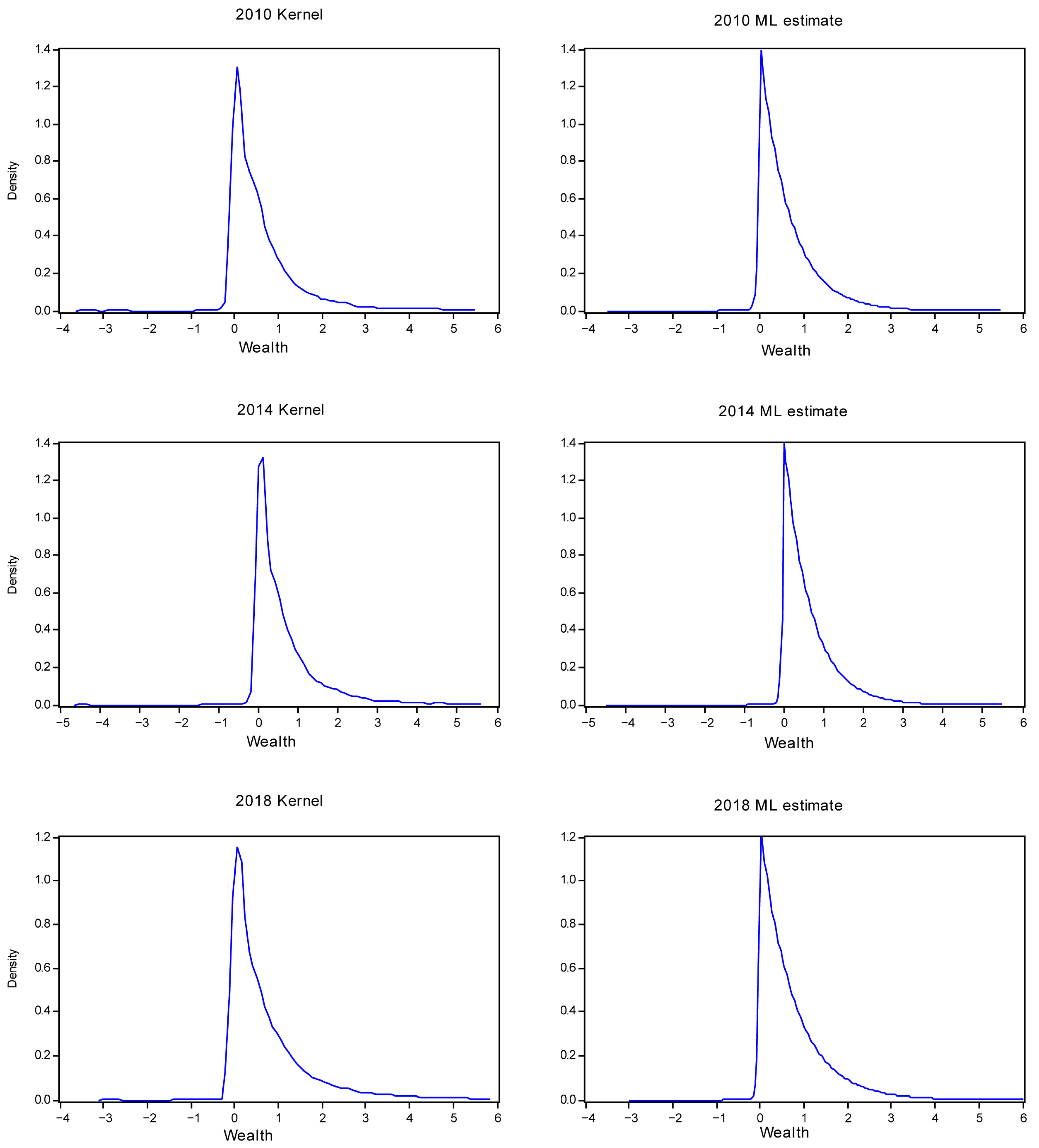
Choosing a suitable parametric distribution to model the wealth data is a difficult problem. The kernel density plots in the left panel of Figure 1 reveal a distribution with a unique shape. None of the distributions that are typically used to model income such as the lognormal, the generalized beta and its special cases, the generalized gamma and its special cases, and the Pareto-lognormal can capture the negative observations and the high concentration of values close to zero6. We began our search for a suitable distribution by trying the generalized extreme value distribution, a distribution which can accommodate negative values and extreme values in the right tail7. However, maximum likelihood (ML) estimates of its parameters produced a density whose shape was a long way from resembling those in Figure 1. In contrast, when we tried the asymmetric Laplace distribution, the ML estimation of its parameters revealed distributions with shapes remarkably like the kernel density estimates. Those distributions are plotted in the right panel of Figure 1. The units of measurement are millions of Australian dollars. The ML-estimated densities have slightly higher peaks than their kernel density counterparts, most likely due to the inability of the ALD to capture a few extreme positive and/or negative values. These discrepancies may impact on our later analysis, but in the absence of a more suitable distribution it is useful to illustrate how the ALD can be used. Later in this paper, in the results section, we compare the ML estimates of the parameters with their posterior means; the means and standard deviations of the observations are also compared with those implied by ML and Bayesian estimation.

Before leaving this section, we provide brief details of ML estimation. Denoting a sample of wealth observations by $\mathbf{x}=\left(x_1,x_2,\dots ,x_N\right)$ and letting $c_i=I(x_i\ge m)$, where $I(.)$ is an indicator function, we can write the log-likelihood function for $\mathsf{\theta }=(m,\lambda ,\kappa )$ as follows:

$$\begin{array}{ll}\hfill L(\mathsf{\theta }|\mathbf{x})& ={\displaystyle \sum _{i=1}^N\ln f(x_i)}\hfill \\ & =N\left[\ln \lambda -\ln \left(\kappa +1/\kappa \right)\right]+\left(\lambda /\kappa \right){\displaystyle \sum _{i=1}^N\left(1-c_i\right)(x_i-m)}-\lambda \kappa {\displaystyle \sum _{i=1}^N{c}_i(x_i-m)}\end{array}$$

(8)

ML estimates for $\mathsf{\theta }$ are obtained by maximizing this function. Hinkley and Revankar (1977) note that the existence of the unknown cut-off point m means that the “classical” regularity conditions for ML estimation are not met, but “generalized classical” regularity conditions do hold, ensuring the estimates have the usual asymptotic properties.

2.4. Computing Dominance Probabilities

The first step towards computing posterior probabilities of dominance is to obtain MCMC samples of the parameters from their posterior densities. We employ uniform and independent priors on all the parameters such that the posterior pdf for $\mathsf{\theta }$ is given by the following:8

$$f(\mathsf{\theta }|\mathbf{x})\propto {\left({\displaystyle \frac{\lambda }{\kappa +1/\kappa }}\right)}^N{\displaystyle \prod _{i=1}^N\left[(1-c_i)\exp \left\{\left(\lambda /\kappa \right)(x_i-m)\right\}+c_i\exp \left\{-\lambda \kappa (x_i-m)\right\}\right]}$$

(9)

For each of the years, 2010, 2014 and 2018, a random walk Metropolis algorithm was used to draw 26,000 observations on $\mathsf{\theta }$ from (9) with the first 1000 treated as a burn-in.9 Let ${\mathsf{\theta }}_X^{(m)},m=1,2,\dots ,M$ and ${\mathsf{\theta }}_Y^{(m)},m=1,2,\dots ,M$ denote two samples of $M=\mathrm{25,000}$ draws for comparing two years identified by the subscripts X and Y. These draws can be used to compute the M quantile and absolute Lorenz curve functions, $Q\left(p,{\mathsf{\theta }}_X^{(m)}\right),$ $Q\left(p,{\mathsf{\theta }}_Y^{(m)}\right),$ $R\left(p,{\mathsf{\theta }}_X^{(m)}\right)$ and $R\left(p,{\mathsf{\theta }}_Y^{(m)}\right),$ $m=1,2,\dots ,M$.

Considering first-order stochastic dominance (FSD) first, the goal is to find the proportion of values of $\left({\mathsf{\theta }}_X^{(m)},{\mathsf{\theta }}_Y^{(m)}\right)$ for which $Q\left(p,{\mathsf{\theta }}_X^{(m)}\right)\ge Q\left(p,{\mathsf{\theta }}_Y^{(m)}\right)$ for all p, as well as the proportion for which $Q\left(p,{\mathsf{\theta }}_X^{(m)}\right)\le Q\left(p,{\mathsf{\theta }}_Y^{(m)}\right)$ for all p. To approximate the requirement that the inequalities hold for all p, we consider 999 values of p from 0.001 to 0.999 at intervals of 0.001. Denote these values as $p_j,j=1,2,\dots ,999$. For the m-th values of ${\mathsf{\theta }}_X$ and ${\mathsf{\theta }}_Y,$ the inequality $Q\left(p_j,{\mathsf{\theta }}_X^{(m)}\right)\ge Q\left(p_j,{\mathsf{\theta }}_Y^{(m)}\right)$ will be satisfied for all values of $p_j$ if

$${\displaystyle \prod _{j=1}^{999}I\left[Q\left(p_j,{\mathsf{\theta }}_X^{(m)}\right)\ge Q\left(p_j,{\mathsf{\theta }}_Y^{(m)}\right)\right]}=1.$$

(10)

Thus, the FSD probability that X dominates Y, equal to the proportion of the M draws for which (10) holds, is given by Equation (11). Similarly, the FSD probability that Y dominates X is given by Equation (12), and subtracting the sum of these two probabilities from one gives the probability of no dominance.

$$\mathrm{Pr}(X\mathrm{dominates}Y)={\displaystyle \frac{1}{M}}{\displaystyle \sum _{m=1}^M{\displaystyle \prod _{j=1}^{999}I\left[Q\left(p_j,{\mathsf{\theta }}_X^{(m)}\right)\ge Q\left(p_j,{\mathsf{\theta }}_Y^{(m)}\right)\right]}}$$

(11)

$$\mathrm{Pr}(Y\mathrm{dominates}X)={\displaystyle \frac{1}{M}}{\displaystyle \sum _{m=1}^M{\displaystyle \prod _{j=1}^{999}I\left[Q\left(p_j,{\mathsf{\theta }}_Y^{(m)}\right)\ge Q\left(p_j,{\mathsf{\theta }}_X^{(m)}\right)\right]}}$$

(12)

$$\mathrm{Pr}(\mathrm{neither}\mathrm{distribution}\mathrm{dominates})=1-\mathrm{Pr}(X\mathrm{dominates}Y)-\mathrm{Pr}(Y\mathrm{dominates}X)$$

For second-order stochastic dominance (SSD), this process is repeated using the functions $R\left(p,{\mathsf{\theta }}_X^{(m)}\right)$ and $R\left(p,{\mathsf{\theta }}_Y^{(m)}\right)$.

A by-product of the estimation procedure is a plot of the following curve

$$P_{X\ge Y}(p)={\displaystyle \frac{1}{M}}{\displaystyle \sum _{m=1}^{M}I\left[Q_X\left(p,{\mathsf{\theta }}_X^{(m)}\right)\ge Q_Y\left(p,{\mathsf{\theta }}_Y^{(m)}\right)\right]}$$

(13)

against the value of p. These curves, which we call probability curves, give the probability of “dominance” at a given population proportion p. The probability of dominance over any range of p will be no greater than the minimum value of $P_{X\ge Y}(p)$ within that range. This characteristic makes $P_{X\ge Y}(p)$ a valuable device for finding the population proportions that have the greatest impact on the probability of dominance.

3. Results and Discussion

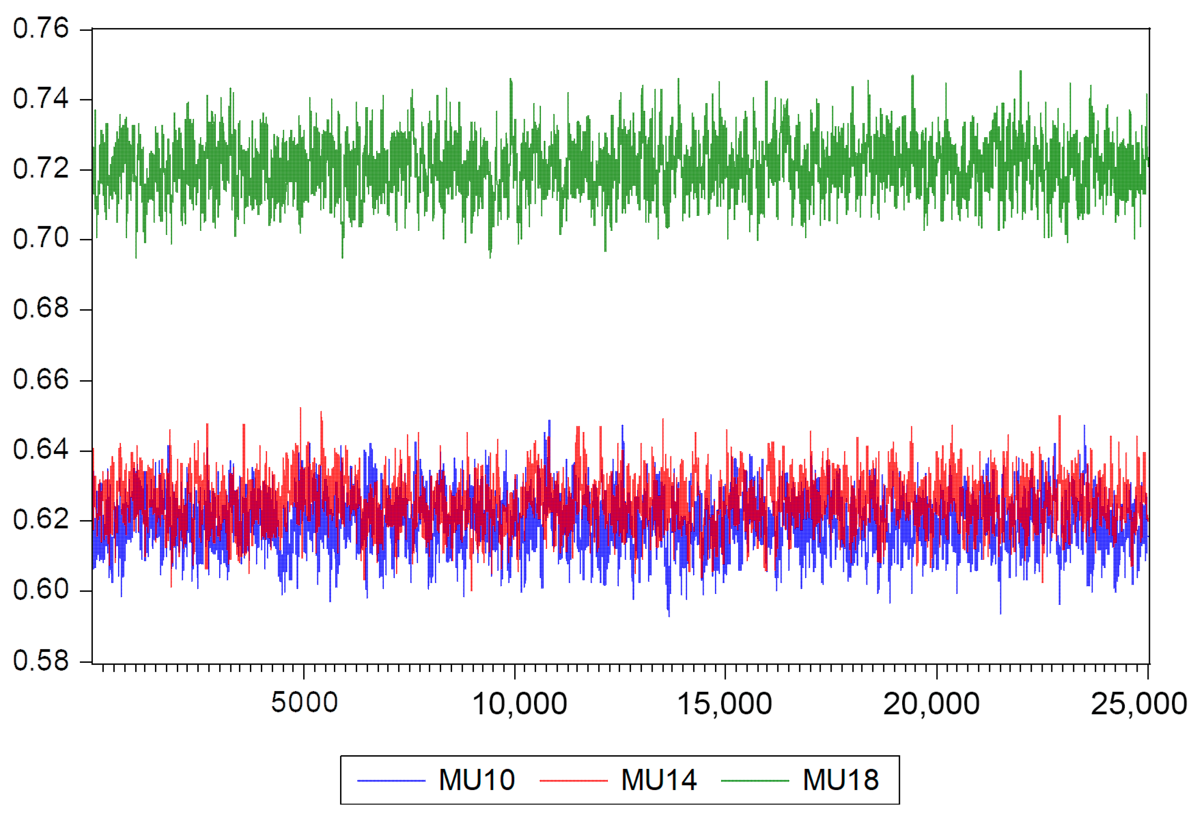
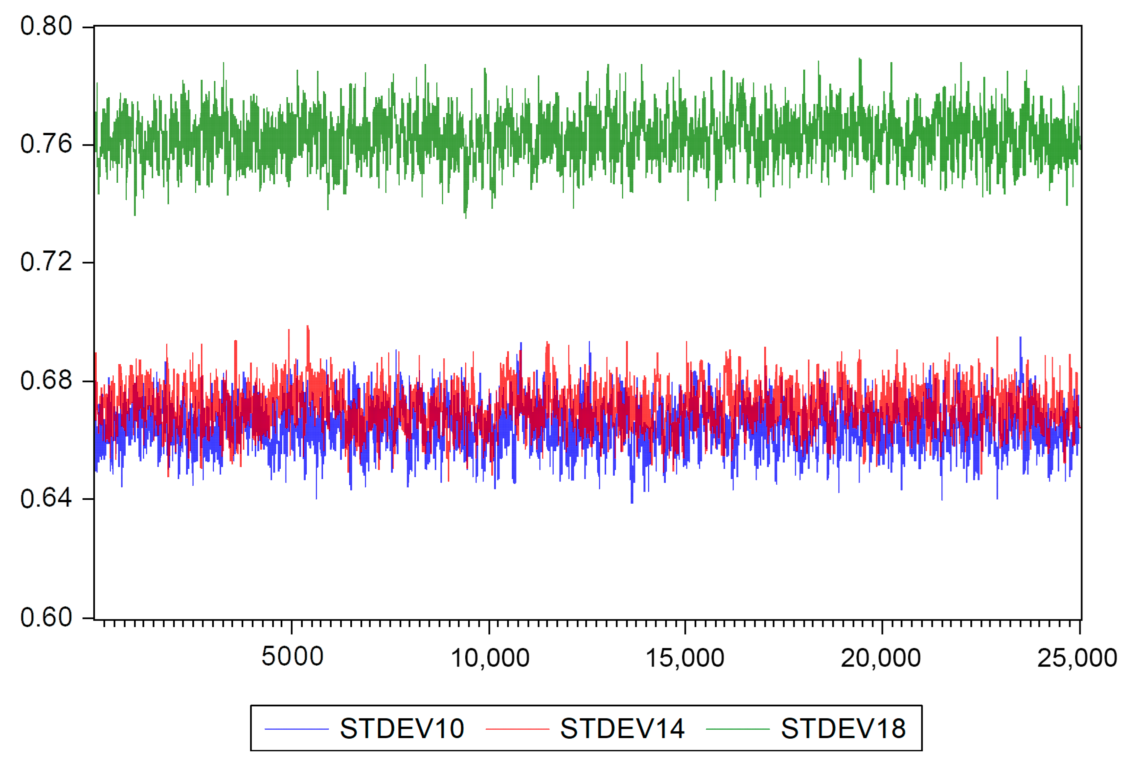
We first consider ML and Bayesian estimates of the ALD parameters and their implied estimates of the means and standard deviations of the distributions. These values are given in

Table 1. Summary statistics, maximum likelihood and Bayesian estimates.

2010
Sample size = 7228
		$\mu$	$\sigma$	m	$\lambda$	$\kappa$
Raw Data		0.6193	0.7967
ML Estimate (Standard Error)		0.6193 (0.0066)	0.6645 (0.0066)	0.0004 (0.0021)	5.8402 (0.0409)	0.2582 (0.0018)
Posterior Mean (Posterior St. Dev.)		0.6195 (0.0076)	0.6647 (0.0077)	0.0006 (0.0007)	5.8401 (0.1116)	0.2583 (0.0045)
2014
Sample size = 9436
		$\mu$	$\sigma$	m	$\lambda$	$\kappa$
Raw Data		0.6254	0.8120
ML Estimate (Standard Error)		0.6254 (0.0057)	0.6710 (0.0058)	0.00001 (0.0018)	5.8198 (0.0358)	0.2566 (0.0016)
Posterior Mean (Posterior St. Dev.)		0.6253 (0.0068)	0.6709 (0.0069)	0.00005 (0.0006)	5.8184 (0.1045)	0.2568 (0.0042)
2018
Sample size = 9523
		$\mu$	$\sigma$	m	$\lambda$	$\kappa$
Raw Data		0.7207	0.9165
ML Estimate (Standard Error)		0.7207 (0.0065)	0.7621 (0.0066)	−0.0003 (0.0019)	5.7248 (0.0416)	0.2295 (0.0017)
Posterior Mean (Posterior St. Dev.)		0.7206 (0.0078)	0.7621 (0.0080)	−0.0006 (0.0007)	5.7435 (0.1114)	0.2289 (0.0040)

Notes: The posterior means and standard deviations were calculated from 25,000 MCMC draws from the asymmetric Laplace posterior pdf. The ML standard errors for $\mu$ and $\sigma$ were calculated from the ML covariance matrix for $(m,\lambda ,\kappa )$ using the delta method.

, along with the means and standard deviations of the raw data. Estimates of the means are almost identical to those from the raw data. The standard deviation estimates are smaller than their raw data counterparts, consistent with our earlier conjecture that the ADL is not capturing a few extreme observations. When we ask how the mean and standard deviation of the wealth has changed from 2010 to 2018, we find little change in both from 2010 to 2014, but a substantial change from 2014 to 2018. In this latter period the level of wealth has increased but inequality has also increased, reflected by the increase in the standard deviation. These characteristics are well depicted by the trace plots for $\mu$ and $\sigma$ in Figure 2 and Figure 3, respectively. These figures serve two purposes. They not only illustrate that $\mu$ and $\sigma$ are similar in 2010 and 2014, and much larger in 2018, but also provide evidence that the MCMCs have converged.

The posterior probabilities for dominance are presented in

Table 2. Posterior probabilities of dominance.

	2010 versus 2014
	Using all quantiles		Using five quantiles
	$FSD$	$SSD$	$FSD$	$SSD$
$\mathrm{Pr}\left({2014}_{SD}2010\right)$	0.3100	0.3474	0.4309	0.3918
$\mathrm{Pr}\left({2010}_{SD}2014\right)$	0.1254	0.1560	0.2003	0.2014
$\mathrm{Pr}\left(\mathrm{no}\mathrm{dominance}\right)$	0.5646	0.4966	0.3688	0.4068
	2014 versus 2018
	Using all quantiles		Using five quantiles
	$FSD$	$SSD$	$FSD$	$SSD$
$\mathrm{Pr}\left({2018}_{SD}2014\right)$	0.9931	0.9915	1.0000	1.0000
$\mathrm{Pr}\left({2014}_{SD}2018\right)$	0.0000	0.0000	0.0000	0.0000
$\mathrm{Pr}\left(\mathrm{no}\mathrm{dominance}\right)$	0.0069	0.0085	0.0000	0.0000

Notes: “Using all quantiles” refers to all quantiles from 0.001 to 0.999 in increments of 0.001. “Using five quantiles” refers to the quantiles 0.1, 0.25. 0.5, 0.75 and 0.9. The dominance probabilities using these quantiles are upper bounds. The corresponding no dominance probabilities are the lower bounds.

. Two sets of probabilities are provided. The first set, labelled “Using all quantiles”, is that obtained using all values of p from 0.001 to 0.999 in increments of 0.001. Assuming this choice of p-values is adequate to represent all p, the probabilities in this set represent the probability that the necessary and sufficient conditions for dominance are satisfied. It is instructive to consider what conclusions might be drawn if a more limited number of values of the cumulative probability p are considered. Comparing these conclusions with those obtained when the complete range of p is considered can indicate the sensitivity of results to the choice of p. Also, satisfying dominance conditions at a limited number of points can be viewed as a set of conditions that are necessary but not sufficient. Resource or data limitations can sometimes mean that checking the necessary conditions is the best we can do. Yitzhaki and Schechtman (2013) argue that it can be useful and instructive to also consider necessary conditions that are not sufficient. As an example of finding posterior probabilities for necessary conditions, we found that the probabilities that (1) and (2) are satisfied at all five quantiles $p^{\ast }=\{0.1,0.25,0.5,0.75,0.9\}$. These probabilities are labelled “Using five quantiles” in Table 2.

Consider first the comparison between 2010 and 2014 using all quantiles. The most likely situation is that neither year dominates. There is weak evidence to suggest 2014 dominates 2010, and even weaker evidence to suggest that 2010 dominates 2014. Because FSD conditions are more restrictive than SSD conditions, we expect the SSD probabilities to be greater than those for FSD. This is indeed the case, but only marginally so. Also, we expect probabilities for conditions which are necessary but not sufficient to be greater than their necessary-and-sufficient counterparts and that is indeed the case when five quantiles are considered. What is perhaps surprising is that the probability for SSD no longer exceeds that for FSD when only necessary conditions are considered. That is, when using five quantiles,

$$\mathrm{Pr}\left({2014}_{FSD}2010|p=p^{\ast }\right)=0.43>\mathrm{Pr}\left({2014}_{SSD}2010|p=p^{\ast }\right)=0.39.$$

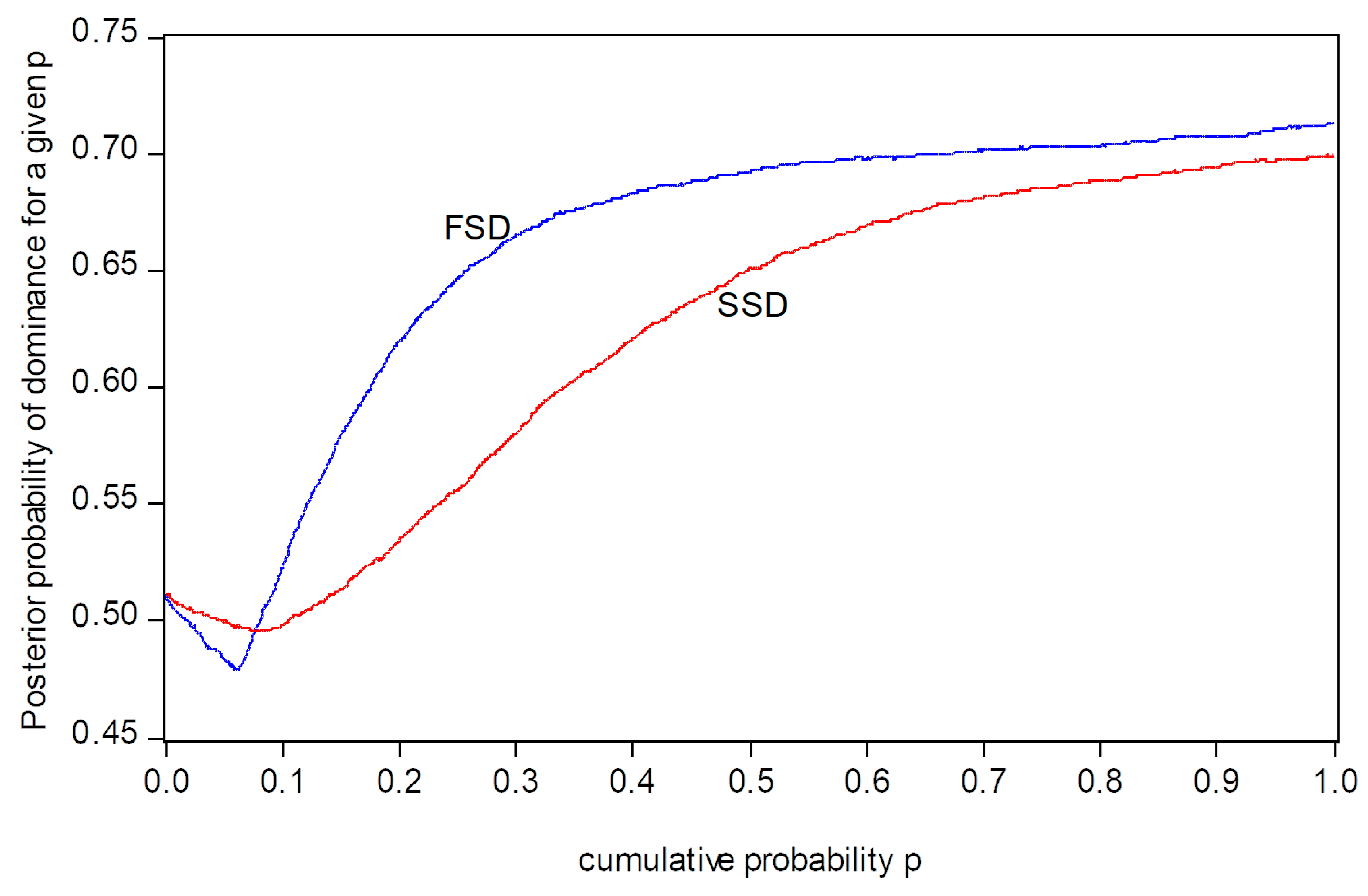
Examining the respective probability curves in Figure 4 provides insights into the relationship. These curves depict $\mathrm{Pr}\left[Q_{2014}(p)\ge Q_{2010}(p)\right]$ and $\mathrm{Pr}\left[R_{2014}(p)\ge R_{2010}(p)\right]$ as functions of p and are labelled FSD and SSD, respectively. Because, for example,

$$\begin{array}{cc}\mathrm{Pr}({2014}_{FSD}2010)& ={\displaystyle \frac{1}{M}}{\displaystyle \sum _{m=1}^M{\displaystyle \prod _{j=1}^{999}I\left[Q\left(p_j,{\mathsf{\theta }}_{2014}^{(m)}\right)\ge Q\left(p_j,{\mathsf{\theta }}_{2010}^{(m)}\right)\right]}}\\ & \le \underset{p}{\min }{\displaystyle \frac{1}{M}}{\displaystyle \sum _{m=1}^{M}I\left[Q\left(p,{\mathsf{\theta }}_{2014}^{(m)}\right)\ge Q\left(p,{\mathsf{\theta }}_{2010}^{(m)}\right)\right]}\end{array},$$

the dominance probabilities must be no greater than the minimum values of the curves. When all values of p are considered, the minimum of the SSD curve is greater than the minimum of the FSD curve. Those minima occur at $p=0.072$ (SSD) and $p=0.062$ (FSD), as depicted in Figure 4. Thus, we obtain the following:

$$\underset{p}{\min }\mathrm{Pr}\left[Q_{2014}(p)\ge Q_{2010}(p)\right]<\underset{p}{\min }\mathrm{Pr}\left[R_{2014}(p)\ge R_{2010}(p)\right].$$

That is,

$$\mathrm{Pr}\left[Q_{2014}(0.062)\ge Q_{2010}(0.062)\right]<\mathrm{Pr}\left[R_{2014}(0.072)\ge R_{2010}(0.072)\right].$$

When the values of p are restricted to $p^{\ast }=\left\{0.1,0.25,0.5,0.75,0.9\right\}$, the minimum values of both curves in Figure 4 occur at $p=0.1$, where

$$\mathrm{Pr}\left[Q_{2014}(0.1)\ge Q_{2010}(0.1)\right]>\mathrm{Pr}\left[R_{2014}(0.1)\ge R_{2010}(0.1)\right]$$

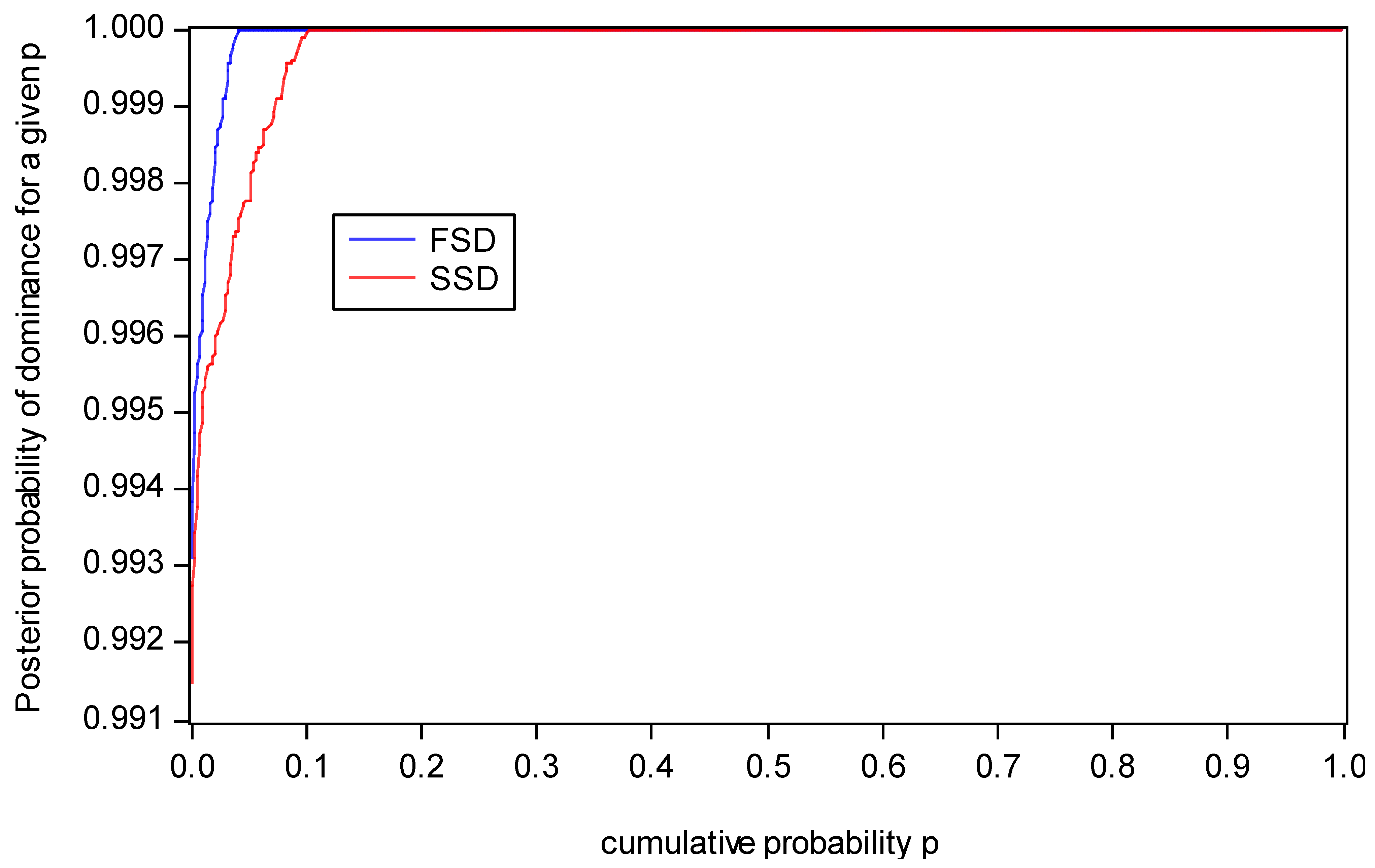
Comparing 2018 with 2014, in Table 2 we find that 2018 dominates 2014 for both FSD and SSD, with all probabilities equal to, or very close to, one. There is a slight anomaly, however. Using all quantiles, the SSD probability of 0.9915 is slightly less than the FSD probability of 0.9931 when we expect it to be larger. Further investigation revealed the problem lies at the zero endpoint. Neither probability curve has an interior minimum. The minimum value for each probability occurs at the smallest value of p. This was confirmed by considering smaller values of p. Eventually the probabilities appear to converge, but at values of p so small their relevance is questionable. The smallest value we considered was $p={10}^{-18}$, which would not include anybody in the current sample. Also, because the calculations involve taking the logarithm of p, there is a high chance of numerical errors. The two probability curves depicted in Figure 5 show that, when $p\ge 0.1$, both the FSD and SSD probabilities are one, a result confirmed by the results from the five quantiles. For $p<0.1,$ the FSD curve is greater than that for SSD and both probabilities of dominance for a given p decline as $p\to 0$. The message to take away from this outcome is that care must be exercised when the minimum of a probability curve is at a boundary point where p equals zero or one. If the smallest and largest values of p considered are 0.001 and 0.999, respectively, and a dominance probability is observed at one of those points, it would be useful to consider smaller or larger values of p to investigate how the dominance probability changes. A judgement about how small or how large these values should be can be based on the sample size.

4. Concluding Remarks

Governments denote considerable resources to monitoring indicators of well-being in the economy. In addition to macroeconomic measures such as the inflation, unemployment and growth rates, there is concern for improvements in attributes such as income, health and education, and the attribute we have considered in this paper: wealth. It is common to use single index measures such as means or medians to indicate whether improvements are being made. These measures do, however, mask what is happening to the complete distribution. The stochastic dominance framework described in this paper is one way of assessing whether there have been improvements over the whole distribution. Presenting information about possible improvements in terms of the posterior probabilities of dominance is more informative than typical sampling theory methods that are characterized by reject/fail-to-reject decisions. The nature of wealth distributions requires careful modelling. We have illustrated how the asymmetric Laplace distribution can be used for this purpose and how posterior dominance probabilities can be computed using it. Our results suggest that, in terms of wealth, society’s welfare did not improve in the period from 2010 to 2014, but from 2014 to 2018 there was a definite improvement. More work is necessary to shed light on what has happened since 2018. Other future research, designed to overcome limitations of the current research, could also be pursued. The modelling of the top coded observations, modifications of the ALD to better capture the peak of the empirical observations, and an investigation into the sensitivity of results when the probability curve minimum is at a boundary are possible candidates.

References

1. Anderson, G. (1996). Nonparametric tests for stochastic dominance. Econometrica, 64, 1183–1193. [Google Scholar] [CrossRef]
2. Barrett, G. F., & Donald, S. G. (2003). Consistent tests for stochastic dominance. Econometrica, 71, 71–104. [Google Scholar] [CrossRef]
3. Bennett, C. J. (2013). Inference for dominance relations. International Economic Review, 54, 1309–1328. [Google Scholar] [CrossRef]
4. Berrendero, J. C., & Cárcamo, J. (2011). Tests for second order stochastic dominance based on l-statistics. Journal of Business and Economic Statistics, 29, 260–270. [Google Scholar] [CrossRef]
5. Bishop, J. A., Chakraborti, S., & Thistle, P. D. (1989). Asymptotically distribution-free statistical inferences for generalized lorenz curves. Review of Economics and Statistics, 71, 725–727. [Google Scholar] [CrossRef]
6. Bishop, J. A., Formby, J. P., & Sakano, R. (1995). Lorenz and stochastic dominance comparisons of european income distributions. Research on Economic Inequality, 6, 77–92. [Google Scholar]
7. Chotikapanich, D., & Griffiths, W. E. (2006). Bayesian assessment of lorenz and stochastic dominance in income distributions. Research on Economic Inequality, 13, 297–321. [Google Scholar]
8. Chotikapanich, D., Griffiths, W. E., Hajargasht, G., Karunarathne, W., & Rao, D. S. P. (2018). Using the GB2 income distribution. Econometrics, 6(2), 21. [Google Scholar] [CrossRef]
9. Davidson, R., & Duclos, J. Y. (2000). Statistical inference for stochastic dominance and for the measurement of poverty and inequality. Econometrica, 68, 1435–1464. [Google Scholar] [CrossRef]
10. Davidson, R., & Duclos, J. Y. (2013). Testing for restricted stochastic dominance. Econometric Reviews, 32, 84–125. [Google Scholar] [CrossRef]
11. Donald, S., & Hsu, Y.-C. (2016). Improving the power of tests of stochastic dominance. Econometric Reviews, 35, 553–585. [Google Scholar] [CrossRef]
12. Gunawan, D., Griffiths, W. E., & Chotikapanich, D. (2021). Posterior probabilities for lorenz and stochastic dominance of australian income distributions. Economic Record, 97(319), 504–524. [Google Scholar] [CrossRef]
13. Gunawan, D., Griffiths, W. E., & Chotikapanich, D. (2023). Comparisons of distributions of australian mental health scores. Australian and New Zealand Journal of Statistics, 65(4), 287–308. [Google Scholar] [CrossRef]
14. Hinkley, D. V., & Revankar, N. S. (1977). Estimation of the pareto law from underreported data, a further analysis. Journal of Econometrics, 5, 1–11. [Google Scholar] [CrossRef]
15. Horváth, L., Kokoszka, P., & Zitikis, R. (2006). Testing for stochastic dominance using the weighted McFadden-Type statistic. Journal of Econometrics, 133, 191–205. [Google Scholar] [CrossRef]
16. Kaur, A., Rao, P. B. L. S., & Singh, H. (1994). Testing for second-order stochastic dominance of two distributions. Econometric Theory, 10, 849–866. [Google Scholar] [CrossRef]
17. Kleiber, C., & Kotz, S. (2003). Statistical size distributions in economics and actuarial sciences. Wiley. [Google Scholar]
18. Koop, G. (2003). Bayesian econometrics. Wiley. [Google Scholar]
19. Kotz, S., Kozubowski, T. J., & Podgórski, K. (2001). The laplace distribution and generalizations: A revisit with applications to communications, economics, engineering and finance. Springer. [Google Scholar]
20. Lambert, P. J. (2001). The distribution and redistribution of income (3rd ed.). Manchester University Press. [Google Scholar]
21. Lander, D., Gunawan, D., Griffiths, W. E., & Chotikapanich, D. (2020). Bayesian assessment of stochastic and lorenz dominance. Canadian Journal of Economics, 53(2), 767–799. [Google Scholar] [CrossRef]
22. Linton, O., Maasoumi, E., & Whang, Y.-J. (2005). Consistent testing for stochastic dominance under general sampling schemes. Review of Economic Studies, 72, 735–765. [Google Scholar] [CrossRef]
23. Linton, O., Song, K., & Whang, Y.-J. (2010). An improved bootstrap test for stochastic dominance. Journal of Econometrics, 154, 186–202. [Google Scholar] [CrossRef]
24. Maasoumi, E., & Heshmati, A. (2000). Stochastic dominance among swedish income distributions. Econometric Reviews, 19, 287–320. [Google Scholar] [CrossRef]
25. Maasoumi, E., & Heshmati, A. (2008). Evaluating dominance ranking of psid incomes by various household attributes. In G. Betti, & A. Lemmi (Eds.), Advances on income inequality and concentration measures (pp. 47–69). Routledge. [Google Scholar]
26. McFadden, D. (1989). Testing for stochastic dominance. In T. B. Fomby, & T. K. Seo (Eds.), Studies in the economics of uncertainty: In honor of josef hadar (pp. 113–134). Springer. [Google Scholar]
27. Reed, W. J., & Jorgensen, M. (2004). The double pareto–lognormal distribution—A new parametric model for size distributions. Communications in Statistics Theory and Methods, 33, 1733–1753. [Google Scholar] [CrossRef]
28. Shorrocks, A. F. (1983). Ranking income distributions. Economica, 50, 3–17. [Google Scholar] [CrossRef]
29. Singh, V. P. (1998). Entropy based parameter estimation in hydrology. Springer. [Google Scholar]
30. Watson, N., & Wooden, M. (2012). The HILDA survey: A case study in the design and development of a successful household panel study. Longitudinal and Life Course Studies, 3(3), 369–381. [Google Scholar]
31. Yitzhaki, S., & Schechtman, E. (2013). The gini methodology: A primer on statistical methodology. Springer. [Google Scholar]
Figure 1. Kernel and maximum likelihood estimates of wealth probability density functions. The left panel contains the kernel estimates and the right panel the maximum likelihood estimates of the asymmetric Laplace distribution.
Econometrics 14 00008 g001
Figure 2. Trace plots of the draws on μ from their posterior distributions.
Econometrics 14 00008 g002
Figure 3. Trace plots of the draws on σ from their posterior distributions.
Econometrics 14 00008 g003
Figure 4. Probability curves for Pr Q 2014 ( p ) Q 2010 ( p )   (FSD) and Pr R 2014 ( p ) R 2010 ( p ) (SSD).
Econometrics 14 00008 g004
Figure 5. Probability curves for Pr Q 2018 ( p ) Q 2014 ( p )   (FSD) and Pr R 2018 ( p ) R 2014 ( p ) (SSD).
Econometrics 14 00008 g005