Econometric Analysis and Forecasts on Exports of Emerging Economies from Central and Eastern Europe

Abstract

This study examines the evolution, heterogeneity, and short-term prospects of export performance in seven Central and Eastern European (CEE) economies—Croatia, Czech Republic, Hungary, Poland, Romania, Bulgaria, and Slovakia—over the period 1995–2024. Using annual World Bank data, exports are modeled as a share of GDP to ensure cross-country comparability and to capture differences in trade dependence. The analysis combines descriptive and inferential statistics with Augmented Dickey–Fuller tests, non-parametric comparisons, Granger causality analysis, and country-specific ARIMA models to investigate export dynamics, the role of foreign direct investment (FDI), and future export trajectories. The results reveal a common long-term upward trend in export intensity across all countries, driven by European integration and structural transformation, but with pronounced cross-country differences in export dependence and volatility. Highly open economies such as Slovakia, Hungary, and the Czech Republic exhibit strong export performance alongside greater exposure to external shocks, while larger domestic markets such as Poland and Romania display lower export intensity and greater stabilization. Granger causality tests indicate that FDI contributes to export growth in several economies, often with multi-year lags, highlighting the importance of absorptive capacity and institutional quality in translating investment inflows into export competitiveness. ARIMA-based forecasts for 2025–2027 suggest continued export expansion and relative stabilization despite recent global disruptions. This study’s primary contribution lies in integrating comparative export analysis, causality testing, and short-term forecasting within a unified econometric framework, offering policy-relevant insights into export-led growth and economic convergence in post-transition European economies.

1. Introduction

International trade has played a key role in the transformation of the former communist economies of Central and Eastern Europe that are members of the European Union, such as the Czech Republic, Slovakia, Hungary, Poland, Romania, Bulgaria, and Croatia, with effects felt in different socio-economic areas. Thus, following the fall of communism, the transition to a market economy in these countries was driven by major economic reforms, with international trade serving as a key engine of economic growth and global integration. Opening to international markets facilitated the inflow of foreign direct investment (FDI), which stimulated infrastructure modernization, industrial development, and job creation. EU membership offered these states access to a vast single market, eliminating trade barriers and supporting export growth (Cieślik et al., 2012). At the same time, it also imposed more rigorous economic and legal standards, helping stabilize the national economies. International trade has allowed these countries to diversify their economies, moving from traditional industries to more competitive sectors, such as IT, the automotive industry, and the production of technological equipment. Exposure to global markets has led local companies to improve the efficiency and quality of their products, thus increasing their international competitiveness. Exports and foreign investment have contributed to GDP growth and trade deficit reduction, strengthening the macroeconomic stability of these states (Gilbert & Muchová, 2018). Thus, international trade has been a key factor in the development of the former communist economies of Central and Eastern Europe, accelerating their modernization and facilitating their integration into the global economy.

After 1990, the evolution of the former communist economies of Central and Eastern Europe—Croatia, the Czech Republic, Hungary, Poland, Romania, Bulgaria, and Slovakia—was marked by their transition to a market economy, structural reforms and European integration. Following the collapse of the communist regimes, these countries experienced a difficult period of economic recession driven by the collapse of central planning, high inflation, and sometimes chaotic privatization processes. In the 1990s, major economic reforms were implemented, such as price liberalization, privatization of state-owned enterprises and attracting foreign investment. The Czech Republic, Hungary, Poland, and Slovakia joined the European Union in 2004, followed by Romania and Bulgaria in 2007 and Croatia in 2013, which brought significant economic benefits, such as access to European funds and markets and an increase in investment. The 2000s was characterized by sustained economic growth, infrastructure development, and increased competitiveness with Slovakia adopting the euro in 2009, consolidating its economic position (Cieślik et al., 2012). The manufacturing sector, especially the automotive industry, has become one of the main engines of economic growth for the Czech Republic, Slovakia, Hungary, Romania, and Poland.

The global economic crisis of 2008–2009 affected most of these countries as well, causing sharp declines in GDP, unemployment, and reduced investment. Hungary and Romania were among the hardest hit, having to request loans from the IMF, while Poland was the only EU country to avoid recession thanks to a more diverse economy and strong domestic consumption. After the crisis, the region’s economies gradually recovered, benefiting from massive European funds, foreign investment, and increased exports. Romania and Bulgaria recorded rapid economic growth, becoming attractive centers for investment, while the Czech Republic and Slovakia consolidated their position in the automotive and IT sectors, becoming highly industrialized economies. On the other hand, Croatia had a slower recovery, but tourism became a key economic driver, while Hungary adopted more nationalist economic policies, focusing on stimulating domestic production and controlling strategic economic sectors.

Moreover, even if the Central and Eastern European economies were hit hard by the COVID-19 pandemic, several countries recovered quickly due to European financial support and increased export demand. Inflation and the 2022 energy crisis have been major challenges, but economies continue to grow thanks to foreign investment and digitalization (Davidescu et al., 2022). Poland, the Czech Republic, and Romania have become important hubs for the relocation of European industry, and Slovakia continues to be a leader in the automotive industry.

The arguments provide evidence the economic transformation of the former communist countries of Central and Eastern Europe has been remarkable, marked by a successful shift from centrally planned systems to dynamic market economies. A pivotal driver of this progress has been their integration into the European Union, which has facilitated structural reforms, investment, and policy alignment; nowadays these countries rank among the most successful emerging economies in Europe.

This study aims to analyze the exports of the emerging economies of Central and Eastern Europe (Croatia, Czech Republic, Hungary, Poland, Romania, Bulgaria, and Slovakia) between 1995 and 2024, using annual export data from the World Bank, modelled using Eviews. The year 1995 was chosen as the starting point of the data set since it was the earliest year in which the World Bank database had export data for all the seven countries. The main objectives include identifying the evolution of exports as a percentage of GDP for each country, comparing export averages and identifying factors that cause these differences. To achieve these objectives, descriptive statistics and the inferential methods were used for the analysis of the export variations, while ARIMA models were used to forecast the exports’ evolution for 2025–2027, aiming to estimate the future tendencies of exports.

Exports are modeled as a percentage of GDP in order to enhance cross-country comparability and to capture the degree of export dependence and trade openness rather than absolute export size. Given the substantial differences in economic scale among the countries analyzed, using export values or volumes would largely reflect country size effects, potentially obscuring structural differences in export orientation and integration into international markets. Expressing exports relative to GDP also reduces the influence of inflation, exchange rate fluctuations, and price-level differences, thereby providing more stable time series for ARIMA modeling over a long historical period. This normalization is particularly relevant in the context of EU integration and convergence analysis, where export intensity is a key indicator of economic openness and external exposure. We acknowledge that modeling exports as a share of GDP may combine movements in both exports and output and may mask sectoral heterogeneity. However, this measure is well suited to the study’s objective of analyzing aggregate export dynamics and generating short-term forecasts of export dependence. Accordingly, the ARIMA forecasts should be interpreted as projections of export intensity rather than absolute export growth.

In order to fulfill its research objective, the paper addresses the following research questions, which structure both the empirical investigation and the discussion of results:

RQ1: Is there a common upward trend in export growth among CEE countries during the period 1995–2024?

RQ2: To what extent do EU integration and foreign direct investment (FDI) inflows influence export performance in the region?

RQ3: Are there significant differences in export performance across individual CEE countries?

RQ4: To what extent does a higher degree of trade openness increase export dependence and volatility, and how does domestic market size mitigate exposure to external shocks in Central and Eastern European countries?

RQ5: Can stable and reliable export forecasts for CEE economies be generated using ARIMA models?

RQ6: Does export growth contribute to the broader process of economic convergence within the region?

These research questions are designed to capture both the structural determinants and the dynamic mechanisms of export evolution in post-transition economies. They replace traditional hypothesis testing with an exploratory, data-driven approach, better suited to the mixed analytical framework combining forecasting, comparative analysis, and causality testing employed in this study.

The novelty of this research consists of carrying out a detailed comparative and updated assessment of export dynamics in seven Central and Eastern European (CEE) countries over nearly three decades (1995–2024), a period that uniquely encompasses the post-COVID recovery and the pre-conflict phase of the Ukraine crisis, as well as pre and post EU ascension phases. Unlike earlier studies that focused on narrower timeframes or single-country analyses, this paper provides a cross-country comparative perspective combining export forecasting with an examination of causal linkages between FDI inflows, EU integration, and trade performance. The inclusion of recent data and short-term forecasts for 2025–2027 allows for a timelier interpretation of export resilience and structural adaptation under evolving geopolitical and economic conditions. This comparative, up-to-date scope represents the paper’s main contribution, distinguishing it from prior studies on post-transition export performance in the CEE region. Rigorous statistical methods are applied, including Shapiro–Wilk, Mann–Whitney, Durbin-Watson, Breusch-Godfrey and ARCH tests to verify the validity of the results. At the same time, the ARIMA based forecasts contribute to understanding future trends and supporting economic and commercial policies.

Beyond examining export dynamics and forecasting trends, this study contributes novel empirical evidence by exploring the causal relationship between foreign direct investment (FDI) inflows and export performance in Central and Eastern European (CEE) economies. Using Granger causality analysis, the paper identifies the direction and timing of interactions between FDI and exports, providing insights into how integration into the European Union and participation in global value chains have shaped the region’s external competitiveness. This approach extends beyond traditional univariate forecasting by linking export evolution to underlying structural and policy-driven mechanisms. In doing so, the study offers a more comprehensive understanding of the factors driving export-led growth in post-transition economies and contributes to ongoing debates on the role of EU integration and investment flows in sustaining long-term economic convergence.

The research paper is structured in several sections. The second section consists of a review of specialized literature, presenting the results obtained by other authors regarding the topics addressed in this paper. The third section presents the research methodology, which includes the main statistical tests used to validate the forecast models, or a comparison of time series, while the fourth section presents and discusses the results of the research carried out in the work, together with the novelty elements. The work ends with the conclusions section and possible further developments.

2. Literature Review

2.1. EU Integration Effects

European integration and trade liberalization have profoundly reshaped CEE export patterns, but with markedly heterogeneous results. Some studies emphasize convergence: for example, Jambor and Gorton (2025) document “convergence clubs” in the region, noting that Poland and the Baltic states leveraged EU accession to achieve rapid agricultural productivity gains and export growth, whereas countries like Hungary and Croatia advanced more slowly. The prevailing trade-growth paradigm (Frankel & Romer, 1999) would predict broad income and export gains from such openness, and indeed CEE countries have seen substantial export-led income convergence. However, other analyses find that rapid integration could also be disruptive for some transition economies. Kuc-Czarnecka et al. (2021) report that the swift trade opening associated with EU enlargement inflicted significant short-term losses on several new members—akin to a sudden “trade shock” that some liken to the Latin American experience of the 1970s. In other words, while accession brought new export opportunities, it also exposed domestic firms to intense competition, producing divergent outcomes across countries.

Empirically, EU and global integration have reoriented CEE trade away from former socialist partners toward Western markets, accompanied by a structural upgrade in exports. For instance, Sheets and Boata (1998) and later Petrova and Sznajder Lee (2024) find that post-2000 export patterns cluster CEE economies into groups: a high-tech manufacturing core (Czech Republic, Hungary, Slovenia, Slovakia) versus a cluster of labor-intensive/resource exporters (the Baltics, Bulgaria), with Poland, Croatia and Romania in between. These observed patterns resonate with standard trade theory. Balassa (1965) introduced the revealed comparative advantage (RCA) index to show how countries specialize in sectors where they hold productivity advantages (Istudor et al., 2022). Indeed, many CEE countries have tended to specialize in industries congruent with their RCA, such as Central Europe in machinery and the Baltics in wood and textiles. Moreover, the Frankel–Romer finding that openness causally raises income suggests that trade integration should bolster growth; the CEE export expansions have certainly been an important engine of GDP growth during the transition (Deij et al., 2018).

At the same time, new trade theories imply more nuanced integration effects. Melitz (2003) shows that liberalization triggers firm-level selection: only the most productive firms export, while smaller firms exit or serve only the domestic market. CEE economies likely experienced such reallocation, though empirical studies directly applying Melitz’s (2003) framework in this context are scarce. Consistent with theory, recent work shows positive spillovers: Șeker and Șimdi (2024) find that a one-country increase in high-tech exports stimulates neighboring CEE exports, indicating integrated supply chains and technology transfer in the region. Monetary integration provides another channel: Cieślik et al. (2012) find that Euro adoption gave a temporary boost by eliminating currency risk for exporters.

While existing literature provides valuable insights into how export patterns in Central and Eastern Europe evolved during integration—such as shifts in destination markets and product composition—it frequently falls short of offering a unified explanation for the underlying drivers of these changes. Notably, there remains a significant gap in studies that simultaneously account for macro-level trade gains, as articulated in the Frankel–Romer framework, and micro-level firm selection dynamics, as theorized by Melitz (2003). This fragmentation narrows the understanding concerning the way in which the dual mechanisms are shaping export performance in transition economies. Furthermore, standard forecasting approaches have yet to incorporate structural indicators such as revealed comparative advantage, leaving models insensitive to changes in specialization or policy shifts. The absence of dynamic forecasting frameworks capable of adjusting to evolving comparative advantages or institutional transformations—such as EU accession or regulatory reform—renders it difficult to anticipate how future phases of integration or disintegration might affect export trajectories in the region.

2.2. Trade Competitiveness and Structural Constraints in Transition Economies

Beyond integration per se, a vast variety of studies examine how trade policies, domestic reforms, and structural factors influence CEE export competitiveness. The consensus is that trade liberalization and institutional quality go hand in hand with improved competitiveness, but structural mismatches persist. For example, Pilinkiene (2016) finds evidence of a virtuous cycle in the region: greater trade openness stimulates GDP growth, which in turn enhances national competitiveness and leads to further export expansion. This suggests that liberalization and regional cooperation have generally been beneficial. Yet domestic conditions are equally important: Davidescu et al. (2022) show that Romania’s export performance depends not only on demand from major EU markets but also on internal factors like government efficiency, corruption control and macroeconomic stability. In practice, CEE countries have had to complement liberal trade policies with institutional reforms to sustain export gains.

Despite these reforms, evidence indicates that CEE exporters face persistent structural competitiveness challenges. Gilbert and Muchová (2018) document that, although CEE transition economies improved their cost competitiveness after EU accession, global market share gains remained modest. The main culprit, they argue, consists of a mismatch between the region’s export profile and fast-growing world demand: CEE has been slow to reorient into new industries, instead largely deepening exports to EU partners. This finding suggests that many CEE countries have continued to rely on goods linked to their static comparative advantage, rather than moving into emerging sectors. Supporting this, Tang (2020) finds that in 1999–2016, exports of fuels and food (lower-value products) contributed to GDP growth in new EU members, while growth from high-value manufactured goods only accelerated later. In other words, although CEE economies have diversified since the 1990s, the timing and composition of exports still reflect old patterns of comparative advantage (Balassa, 1965) rather than a fully modernized export base.

At the micro level, firm- and sector-specific constraints hinder competitiveness. Melitz’s (2003) insight implies that only the most productive firms can exploit foreign markets In CEE, some evidence hints at such selection effects. Giucă et al. (2024) report that Romania’s vegetable sector suffers a chronic trade deficit because its farms are small, fragmented and technologically lagging, failing to meet the scale or quality needed to compete internationally. By Melitz’s (2003) logic, these inefficient producers will exit if markets fully open. Yet policy has not always facilitated this process. More generally, many studies note that investment in R&D, innovation, and infrastructure (factors underlying higher productivity) remain below what is needed for global competitiveness, even after years of convergence.

External shocks have further tested competitiveness. Notably, Kos-Labedowicz and Talar (2024) examine the Russia–Ukraine war and find that trade exposure did not uniformly translate into collapse: countries deemed “vulnerable” (e.g., Slovakia, Czech Republic) maintained robust exports in 2022 despite the conflict. This resilience implies that factors such as diversified trade networks or adaptive firms can mitigate price-based competitiveness deficits. It also underscores that conventional measures of competitiveness—which focus on costs and productivity—may miss dynamics like supply-chain flexibility.

Although a substantial body of literature has identified the key determinants of export competitiveness—such as trade openness, institutional quality, and technological capacity—these factors are rarely connected in a systematic way to forecasting outcomes. Comparative or counterfactual analyses across Central and Eastern European economies remain scarce, leaving unclear which structural constraints most significantly hinder export performance. Moreover, despite the relevance of classical trade concepts like revealed comparative advantage and modern firm-level theories such as Melitz’s (2003) model of heterogeneous exporters, these frameworks have not been rigorously incorporated into quantitative competitiveness indices tailored to the region. This omission limits the development of a coherent, data-driven understanding of the primary bottlenecks affecting export potential. In current forecasting practices, competitiveness is often treated as a static or exogenous condition, rather than as an evolving, measurable factor. As a result, most export projections fail to account for critical scenarios—such as declining institutional quality or shifts in comparative advantage—that could substantially reshape future export trajectories in transition economies.

2.3. Export-Led Growth and Value Chains

A wide range of statistical methods have been applied to forecast exports and trade-related indicators, but few are tailored to the CEE transition context. The foundational approach is autoregressive time-series modeling (see, for instance, Popescu et al., 2025). ARIMA models, for example, excel at capturing trends and seasonality in trade data. Lima et al. (2024) find ARIMA consistently outperforms Holt–Winters exponential smoothing for European retail trade forecasts. Similarly, Toaca et al. (2025) prove that an ARIMA model augmented with seasonal dummies closely tracked Moldova’s monthly export volatility, significantly reducing errors relative to naive benchmarks. Simple extrapolation can also be effective when trends are stable: Stankov et al. (2023) achieved an R² above 0.9 by fitting linear trends to Serbia’s fruit trade, projecting continued export growth based on historical patterns. These results illustrate that as far as short-term forecasting is concerned, well-specified classical models remain powerful, especially when historical seasonality and trends dominate.

Researchers also find benefit in combining models or using multivariate extensions. Toaca et al. (2025) note that averaging several ARIMA forecasts can lower error compared to relying on a single specification. In volatile series, adding volatility components (e.g., GARCH) can improve precision: Mahmoud Sayed Agbo (2023) enhances ARIMA forecasts of Egypt’s agricultural export prices by modeling time-varying variance.

Beyond traditional statistics, machine-learning methods have gained traction for capturing non-linear trade dynamics. For instance, Dai (2023) employs a neural network that predicts export volumes with over 30% greater accuracy than conventional regression and time-series models, thanks to its ability to learn complex relationships among macro indicators. Karabay et al. (2023) apply a neural-network autoregressive model to Turkey’s apparel exports and likewise find out it outperforms ARIMA approaches on standard error metrics. These studies suggest AI-based methods can uncover subtle patterns or structural breaks in the data that linear models miss. However, this power comes with costs: machine-learning models typically require large data samples and often sacrifice interpretability in terms of quality. Toaca et al. (2025) explicitly warn that methods like recurrent neural networks, although flexible, demand more data and obscure economic relationships compared to classic models.

Another emerging approach is to incorporate survey- or sentiment-based indicators. Lehmann (2021) shows that forward-looking business and consumer survey measures—such as export order books and industrial confidence—significantly improve short-term export forecasts for European countries. In out-of-sample tests for 18 economies, models including these “soft” indicators consistently yield lower errors for export growth than pure autoregressive benchmarks. This implies that qualitative expectations data can help to anticipate turning points in export performance that lagging indicators might miss.

Despite recent methodological advances in trade forecasting, their application to Central and Eastern European transition economies remains notably limited. Existing studies tend to focus on broader or non-comparable contexts—such as Egypt, Turkey, or Western Europe—failing to account for the unique structural and historical characteristics of post-socialist CEE countries. Most forecasting models overlook critical discontinuities in relation to EU accession, large-scale privatization, and region-specific external shocks, all of which have played a defining role in shaping export dynamics. Moreover, current approaches rarely integrate the theoretical foundations provided by the trade economics literature. A robust forecasting framework for CEE would ideally incorporate evolving comparative advantages and productivity shifts—elements central to models such as Melitz’s (2003)—yet these factors are typically treated as static or exogenous. Consequently, there remains a significant gap in developing export forecasting models that are both methodologically rigorous and contextually grounded in the institutional and structural realities of CEE economies. Until such frameworks are developed, the capacity to accurately project export trajectories in light of the region’s transitional legacies and ongoing economic transformations remains constrained.

Recent advances in econometric methodology have emphasized the importance of distributional heterogeneity and tail-dependent relationships in economic analysis. In this context, Ul-Durar et al. (2025) provide a comprehensive survey of quantile regression applications, highlighting how economic relationships may differ across the conditional distribution of the dependent variable and how tail behavior can reveal asymmetric or non-linear effects that are obscured by mean-based approaches. Their framework is particularly relevant for analyzing inequality, risk transmission, and heterogeneous responses to economic shocks.

While such distribution-sensitive techniques offer valuable insights, the present study departs from this strand of literature by focusing on the temporal dynamics and aggregate evolution of exports rather than on conditional distributional effects. Specifically, this paper employs ARIMA models to capture persistence, trend behavior, and short-term predictability in export intensity, complemented by Granger causality tests to examine the dynamic interaction between foreign direct investment and exports. This time-series–oriented approach is well suited to the study’s objective of generating policy-relevant export forecasts and identifying medium-term transmission mechanisms in post-transition economies. Consequently, our contribution is complementary to quantile-based analyses: instead of modeling heterogeneity across the export distribution, we emphasize cross-country comparability, dynamic adjustment, and forecasting performance in the context of European integration and structural transformation.

2.4. International Trade Theories

A solid theoretical foundation links export growth to economic transformation. For example, classic trade-growth models highlight that a country’s comparative advantage evolves over time through technology and factor accumulation (Fertő, 2007). In this view, economies specializing in the “wrong” industries can suffer permanently by a slower growth (Grossman & Helpman, 1991; Lucas, 1988). Applied to CEE, this implies exports should shift from low-tech or primary goods towards more complex industries as countries develop (Bierut & Kuziemska-Pawlak, 2016). New Trade Theory (Krugman, 1980) and firm-level models (Melitz, 2003) add that reducing trade barriers (e.g., EU accession) leads only the most productive firms to export and forces inefficient ones to exit, raising industry productivity. In short, as trade costs fall, firms reallocate towards export sectors and aggregate productivity rises (Melitz, 2003). Convergence theory also suggests that poorer CEE economies should experience faster catch-up growth once they integrate with richer markets (Borys et al., 2008). These theories jointly predict that EU integration and increased competition will spur a deepening and upgrading of CEE exports.

Empirical gravity models show trade volumes are largely driven by market size and proximity. EU enlargement removed tariffs and barriers, effectively enlarging market size. Indeed, studies find CEE countries have rapidly expanded trade with the euro-area, becoming its third-largest partner, driven by geographic closeness and growth. In this context, participating in the EU’s Customs Union creates trade-creation: CEE exporters gain easier access to large EU markets at lower cost (Borys et al., 2008). New-Economic-Geography models predict that when trade costs fall, industry relocates toward core markets, potentially producing a “core-periphery” pattern (Székely & Kuenzel, 2021). In practice, EU membership and free-trade agreements have indeed been associated with significantly higher trade and investment flows between CEE and Western Europe (Bussière et al., 2005).

As noted above, comparative advantage is dynamic as argued by Fertő (2007), who finds that while some new EU members continued to specialize in traditional sectors, others (Poland, Hungary, Czech Republic, Slovenia) have upgraded their revealed comparative advantage toward technology- and human-capital-intensive product. In combination, these theories predict catch-up export growth in CEE driven by structural shifts to higher-value goods.

Moreover, according to Melitz (2003), exposure to larger markets and competition causes only the most efficient firms to export; the rest exit, raising average productivity. In a CEE context, EU accession and deeper integration mean firms face bigger markets and must upgrade productivity to survive. Relatedly, Krugman’s (1980) models of integration suggest gains from scale economies and agglomeration when barriers fall (Székely & Kuenzel, 2021). These mechanisms imply that trade liberalization linked with EU integration should lead to productivity gains and thus stronger export performance.

Beyond trade costs, recent studies emphasize non-price factors. Bierut and Kuziemska-Pawlak (2016) show that CEE export shares grew substantially over two decades, largely driven by technological innovation and institutional quality rather than mere cost-competitiveness. In their panel analysis, patenting (innovation) had the strongest positive effect on export performance, and improvements in regulatory quality also boosted market shares. This suggests that as CEE firms adopt new technologies and as institutions improve through EU norms, exports expand and become more sophisticated (Bierut & Kuziemska-Pawlak, 2016).

While international trade theories offer robust conceptual frameworks for understanding the evolution of export structures in transition economies, their empirical application to Central and Eastern Europe (CEE) remains fragmented and underdeveloped. Existing studies often treat classical, new trade, and firm-level theories in isolation, without integrating their mechanisms into a unified analytical or empirical framework. For example, while the Melitz model has been widely cited to explain post-accession firm dynamics, few studies have operationalized its predictions using firm-level export data across CEE. Similarly, the evolving nature of comparative advantage is well established theoretically, yet seldom linked to forecasting models or sector-specific policy assessments in the region. There is also a lack of longitudinal studies that connect the theoretical predictions of export upgrading, market reallocation, and productivity convergence with real-time structural indicators or trade policy changes. As a result, the capacity to translate theoretical insights into predictive tools that capture the complexity of CEE’s export transformation remains limited, leaving a significant gap in theory-informed forecasting for post-transition economies.

2.5. EU Integration, FDI, and Export Growth

After 2004, EU accession was expected to accelerate these trends. Removal of tariff and non-tariff barriers under the EU framework gave CEE firms direct access to western markets. Several studies find a marked increase in trade around EU entry: for example, ECB analysis shows CEE integration with the euro-area doubled in the 1990s and continued into the 2000s, driven by proximity, growth differentials, and especially by “removal of trade hurdles and accession to the European Union” (Bussière et al., 2005). In theory, joining the EU also commits countries to legal and regulatory reforms, which can raise investor confidence and trade integration.

Foreign direct investment (FDI) is a key channel connecting integration to exports. Western European multinationals invested heavily in CEE after EU enlargement, bringing new technologies and integrating local plants into EU-wide supply chains (Jirasavetakul & Rahman, 2018; Székely & Kuenzel, 2021). This FDI inflow was both motivated by new market access and helped CEE countries move into higher-value sectors. Indeed, IMF research finds EU-11 member states (joined 2004+) received about $700 billion in FDI by 2016, and that FDI “has played a strong role in the export-led growth of Eastern European countries” (Jirasavetakul & Rahman, 2018). Over time, these investments reshaped CEE export baskets towards more technology-intensive products. In short, EU accession increased FDI, and FDI in turn boosted exports and moved them up the value chain.

Moreover, empirical work confirms that EU accession itself raised growth factors that support exports. One cross-country study finds EU membership had a “strong positive impact on FDI inflows,” reflecting both the trade benefits and structural reforms associated with accession (Jirasavetakul & Rahman, 2018). Another strand of regional integration literature predicts that customs union membership creates trade among member states at the expense of non-member states, consistent with CEE export patterns shifting towards EU partners. Therefore, the post-2004 era saw CEE economies rapidly integrate: EU markets became dominant destinations, and FDI-led supply-chain embedding enabled sustained catch-up via exports (Bussière et al., 2005; Gábor Márk Pellényi, 2020).

Although extensive research has documented the positive relationship between EU integration, foreign direct investment, and export growth in Central and Eastern Europe, several analytical gaps persist. Most existing studies focus on the descriptive effects of integration—such as increases in trade volume and FDI inflows—without fully disentangling the causal pathways through which these forces influence export sophistication and sustainability. The role of FDI in reshaping export structures is often acknowledged but rarely modeled with precision, particularly in terms of how technology transfer, supply chain embedding, and ownership structure affect long-term competitiveness. Furthermore, the integration–FDI–export nexus has not been sufficiently incorporated into forecasting frameworks. There is a notable absence of dynamic models that can simulate how future shifts in EU policy, investment trends, or geopolitical shocks might alter export trajectories. Consequently, a critical gap remains in developing forward-looking approaches that account for the structural role of FDI and institutional integration in shaping the export futures of CEE economies.

3. Research Methodology

The application of both descriptive and inferential statistical techniques facilitates a comprehensive examination of economic and financial data, allowing for the derivation of insights that support informed decision-making. At the same time, rigorous empirical analysis requires careful consideration of contextual conditions and the selection of analytical methods that are consistent with the characteristics and distributional properties of the underlying data.

The normality of the analyzed time series is evaluated using the Shapiro–Wilk test, which is particularly appropriate for small samples, typically those containing fewer than 50 observations. At the conventional 5% significance level, a probability value exceeding 0.05 indicates that the null hypothesis of normality cannot be rejected. For a time series Y_t, where t = 1, …, n, the Shapiro–Wilk statistic, as introduced by Shapiro and Wilk (1965), provides a formal measure for assessing whether the observed distribution deviates from normality:

$$W={\displaystyle \frac{{\sum }_{t=1}^n{(p_t y_t)}^2}{{\sum }_{t=1}^n{(y_t-\overline{y})}^2}},$$

(1)

where y_t denotes the ordered observations of the original series Y_t, arranged in ascending order y₁ ≤ y₂ ≤ … ≤ y_n represents the sample mean, and p_t are the associated weighting coefficients. The null hypothesis of normality is rejected when the test statistic WWW is less than or equal to the critical value W_α, as reported by Shapiro and Wilk (1965) for the selected significance level. In addition, the procedure provides a corresponding probability value, computed using IBM SPSS Statistics 31.0; a probability greater than 0.05 indicates that the null hypothesis of normality cannot be rejected at the 5% significance level.

The Mann–Whitney test—also referred to as the Mann–Whitney U test or the Wilcoxon rank-sum test (Mann & Whitney, 1947)—is a non-parametric procedure used to compare two independent samples and to evaluate whether they originate from the same underlying distribution. It serves as a suitable alternative to the independent-samples t-test when the assumption of normality is violated. Under the null hypothesis H₀, the distributions of the two groups are assumed to be identical, whereas the alternative hypothesis H₁ posits the existence of a statistically significant difference between them. The test yields the U statistic, which quantifies the extent of divergence between the sample distributions, together with an associated probability value that reflects the likelihood that the observed differences arise by chance. A p-value below 0.05 leads to rejection of the null hypothesis and indicates a statistically significant difference between the samples; conversely, a p-value above this threshold suggests insufficient evidence to conclude that the distributions differ.

To estimate the parameters of the ARIMA forecasting models, the least squares estimation technique was applied. The statistical significance of individual coefficients was assessed using Student’s t-test, while the overall validity of each model was evaluated through the F-test. The null hypothesis H₀ assumes that the estimated coefficients are not statistically different from zero, whereas the alternative hypothesis H₁ indicates statistically significant parameters. When the probability values associated with the t- and F-statistics fall below the 0.05 threshold, the null hypothesis is rejected in favor of H₁ at the 5% level of significance.

Subsequently, a series of diagnostic tests is applied to verify the adequacy of the estimated models. First-order serial correlation and the independence of residuals are examined using the Durbin–Watson test, while higher-order autocorrelation is assessed through the Breusch–Godfrey test. In addition, the ARCH test is employed to evaluate whether the variance of the error terms is constant over time or exhibits conditional heteroscedasticity. Autocorrelation arises when residuals are correlated across time, which may result in underestimated standard errors and, consequently, misleading inferences regarding parameter significance. The Durbin–Watson statistic (DW) is computed based on the differences between residuals observed in successive time periods (Durbin & Watson, 1950)

$$DW={\displaystyle \frac{{\sum }_{i=2}^n{(e_i-e_{i-1})}^2}{{\sum }_{i=1}^n{\left(e_i\right)}^2}}$$

(2)

where n denotes the total number of observations. The Durbin–Watson statistic takes values between 0 and 4, with values close to 2 indicating the absence of first-order autocorrelation in the residuals. In practical applications, the calculated DW value is compared against the lower d_L and upper d_U critical bounds provided in the Durbin–Watson tables for the chosen significance level. When the statistic lies within the interval (d_u, 4 − d_u) the null hypothesis H₀ of no residual autocorrelation is accepted.

The Breusch–Godfrey test (Breusch, 1978; Godfrey, 1978) is applied to identify the presence of higher-order serial correlation in the model residuals and yields a corresponding probability value. When this probability is greater than 0.05, the null hypothesis H₀ cannot be rejected, indicating that higher-order autocorrelation is not statistically significant at the 5% significance level.

The Dickey–Fuller test (Dickey & Fuller, 1979) is employed to assess whether a time series is stationary, a fundamental requirement in time-series analysis. Stationarity implies that key statistical properties of the series, such as its mean and variance, remain constant over time. The test examines the presence of a unit root within an autoregressive framework, where the existence of such a root indicates non-stationarity. In this case, the series exhibits persistent movements over time and does not revert to a stable long-run mean. To enhance robustness, the augmented Dickey–Fuller (ADF) test is used, allowing for the inclusion of deterministic components (such as an intercept or trend) and additional lagged terms. These lagged differences serve to eliminate residual autocorrelation, which may otherwise bias inference when applying the basic Dickey–Fuller test. The null hypothesis H₀ posits the presence of a unit root, while the alternative hypothesis H₁ implies stationarity of the series. Test outcomes are interpreted by comparing the calculated test statistic with critical values at the 1%, 5%, and 10% significance levels, or by evaluating the associated probability value. A probability below 0.05 leads to rejection of the null hypothesis, indicating that the time series is stationary at the 5% significance level.

The ARCH test (Engle, 1982) is applied to identify the presence of conditional heteroscedasticity in time-series data. Heteroscedasticity arises when the variance of the regression residuals is not constant over time; in a conditional setting, this variance depends on past error terms. The null hypothesis H₀ assumes that the residual variance is homoscedastic and remains stable across periods, whereas the alternative hypothesis H₁ indicates that the variance is conditionally time-dependent. The test yields an associated probability value, and when this value exceeds 0.05, the null hypothesis is not rejected, implying the absence of conditional heteroscedasticity at the 5% significance level.

The ARIMA (AutoRegressive Integrated Moving Average) model is a widely used statistical framework for time-series analysis and forecasting, denoted as ARIMA(p,d,q). The model integrates three core components (Box et al., 2016). The autoregressive (AR) component captures the dependence of the current value of the series on its past realizations, with the parameter p indicating the number of lagged terms included. The integrated (I) component reflects the degree of differencing required to render the series stationary, where the parameter d specifies the number of times the series must be differenced to remove deterministic trends. Finally, the moving average (MA) component accounts for the influence of past forecast errors on current values, with the parameter q representing the number of lagged error terms incorporated into the model.

4. Results

4.1. Export Dynamics in CEE Countries

The evolution of exports in Central and Eastern European (CEE) countries between 1995 and 2024 reflects the profound economic transformations resulting from the transition from centrally planned to market economies, driven by trade liberalization, foreign direct investment, and European integration. In the first stage (1995–2007), export growth was primarily driven by specialization in medium-technology manufacturing industries, supported by relatively low labor costs and capital accumulation, which facilitated technological modernization and productivity improvements. This trajectory is consistent with international trade and economic convergence theories, which emphasize the role of factor endowments and the adoption of advanced technologies in approaching the efficiency levels of developed economies.

In the subsequent stage (2007–2015), the progressive accession of CEE countries to the European Union accelerated trade flows and structural reorganization, fostering integration into global value chains and strengthening external competitiveness, while cross-country differences were shaped by the timing of accession and the specific characteristics of infrastructure and industrial policies.

In the most recent period (2016–2024), exports reflected the maturation of competitive advantages and structural adjustment to global factors, such as supply chain reconfigurations, the global health crisis, and geopolitical tensions. Within this context, the Czech Republic, Slovakia, and Hungary experienced rapid export growth due to early integration and robust industrial infrastructure; Poland pursued a strategy of diversification and consolidation of domestic exporters; and Romania, Bulgaria, and Croatia exhibited later or more fluctuating developments, consistent with slower transitions and less developed infrastructure. Overall, the dynamics of CEE exports confirm the role of international trade, economic convergence, and regional integration in structural modernization and the gradual convergence of these economies toward the development levels of Western European states, highlighting the direct link between economic policies, institutional context, and external performance in the region.

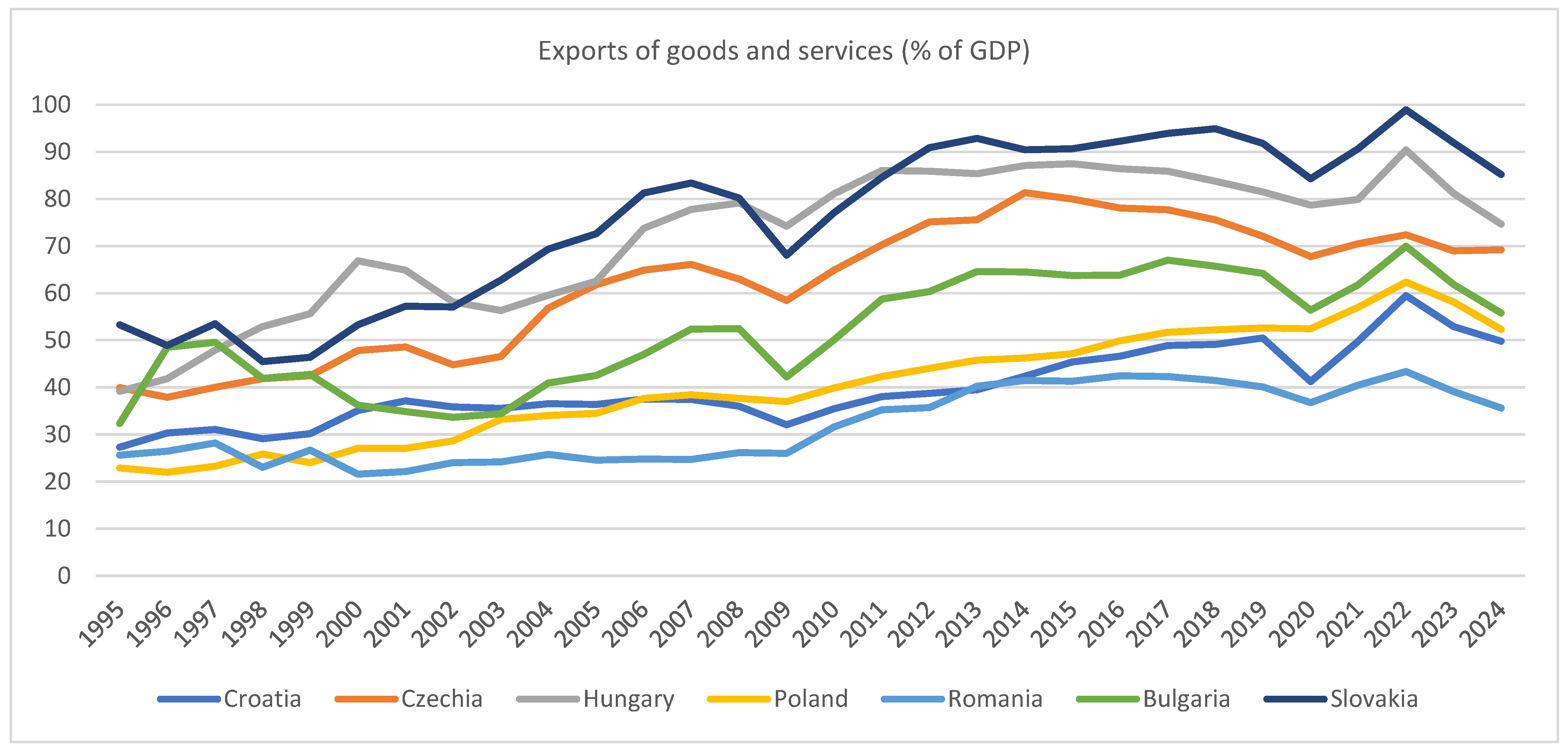
The Central and Eastern European countries experienced a visible increase (Figure 1) in the export share in GDP during the transition period, as a result of EU accession (2004–2007) and the inflow of foreign investment. Slovakia, Hungary, and the Czech Republic stand out with very high values (often above 70–90% of GDP), explained by export-oriented markets integrated into European value chains (especially the automotive and electronics industries). Romania and Poland show lower values (20–45% for Romania, 20–60% for Poland), reflecting larger domestic markets, less dependent on exports. At the same time, Bulgaria and Croatia are at an intermediate level (40–65%), with Bulgaria’s exports increasing after 2004, driven by investment and EU integration.

The global financial crisis (2008–2009) caused notable declines in all countries (e.g., Hungary from 79% in 2008 to 74% in 2009; Romania from 52% to 42%), primarily due to decreased external demand in key sectors such as automotive and capital goods. Between 2010 and 2014, a post-crisis recovery led to significant increases, especially in the Czech Republic, Slovakia, and Hungary. The period 2015–2019 was marked by relative stagnation and structural adjustments, with slower growth in countries with strong domestic markets, such as Poland and Romania. The COVID-19 pandemic in 2020 generated sharp declines (Romania 36%, Croatia 41%, Czech Republic 67%) due to restrictions, supply chain disruptions, and reduced external demand, followed by strong rebounds in 2021–2022 (e.g., Slovakia 99%, Hungary 90%) driven by recovering global demand and industrial production. In 2023–2024, most countries experienced declines linked to the European economic slowdown, high inflation, and the impact of the war in Ukraine.

Differences in export performance reflect structural characteristics. Highly open markets such as Slovakia, Hungary, and Czech Republic depend heavily on industrial exports, particularly in the automotive sector, making them sensitive to cyclical European and global dynamics. Medium-open markets, including Bulgaria and Croatia, combine tourism, industry, and services, showing growth aligned with EU integration but subject to seasonal variations. Larger markets with substantial domestic markets, such as Poland and Romania, record lower export shares, as domestic consumption partially offsets dependence on external trade.

These differences can be observed in

Table 1. Descriptive statistics of exports (% of GDP).

	Mean	Standard Deviation	Coefficient of Variation	Kurtosis	Skewness	Minimum	Maximum
Croatia	39.85%	7.99%	20.05%	−0.27	0.60	27.306%	59.49%
Czech Republic	62.02%	13.84%	22.32%	−1.20	−0.45	37.89%	81.35%
Hungary	72.21%	14.78%	20.47%	−0.51	−0.79	39.18%	90.41%
Poland	40.24%	11.83%	29.41%	−1.13	0.02	21.98%	62.35%
Romania	32.03%	7.70%	24.06%	−1.74	0.16	21.58%	43.36%
Bulgaria	52.02%	11.65%	22.40%	−1.30	−0.22	32.33%	69.97%
Slovakia	76.12%	17.15%	22.53%	−1.24	−0.52	45.48%	98.95%

Source: Authors’ contribution, based on data from the World Bank (Exports of Goods and Services).

, where Slovakia (76.1%), Hungary (72.2%), and Czech Republic (62.0%) register the highest average export share in GDP, confirming their status as highly export-oriented economies. At the opposite end of the spectrum, Romania (32.0%) and Croatia (39.8%) exhibit markedly lower levels of export dependence, while Poland (40.2%) and Bulgaria (52.0%) register intermediate values. These values align with the broader regional pattern in which Central European economies—characterized by advanced industrial structures and stronger integration within EU production systems—display significantly higher export intensity compared to Southeastern European economies, where export growth has progressed more gradually due to structural and institutional constraints.

Czech Republic (13.8%), Hungary (14.8%), and Slovakia (17.1%) record the largest standard deviations in export shares, indicating substantial year-to-year variability and a strong sensitivity to external economic cycles. In contrast, Romania (7.7%) and Croatia (8.0%) display smaller deviations, suggesting relatively greater stability, although at lower levels of export intensity. This pattern is further supported by the coefficient of variation, which shows that Poland (29.4%) and Romania (24.1%) have the most unstable series relative to their average export levels, while Croatia (20.0%) and Hungary (20.5%) exhibit comparatively more consistent export behavior over time.

Overall, the evidence confirms that Slovakia, Hungary, and the Czech Republic represent highly open but more volatile economies, whose export performance remains closely tied to industrial sectors—particularly the automotive and electronics industries—and thus to broader European demand cycles. By contrast, Romania and Poland maintain lower export-to-GDP ratios, with fluctuations that appear more pronounced relative to their average levels; this can be attributed to the stabilizing role of their large domestic markets, which cushion external shocks. Bulgaria and Croatia occupy an intermediate position, characterized by more diversified export structures and flatter distributions, reflecting a balanced mix of industrial, service, and tourism-based economic activities that help moderate volatility.

The differences in export performance among the analyzed CEE countries can be attributed to a complex interplay of economic structure, industrial specialization, foreign investment policies, and infrastructural development. Countries such as Slovakia, Hungary, and the Czech Republic record the highest export shares (exceeding 60% of GDP), largely due to their deep integration into European production networks, particularly in the automotive and machinery industries (e.g., Volkswagen, Audi, Škoda). In contrast, Romania and Croatia display considerably lower average export shares (32.03% and 39.85%, respectively), reflecting a smaller industrial base and more limited participation in Central European supply chains. Economies with smaller domestic markets, such as Slovakia and Hungary, tend to exhibit higher export dependence, whereas Poland and Romania, with larger and more diversified internal markets, rely more heavily on domestic consumption, thereby reducing export intensity. Policy differences have also played a crucial role: Hungary, the Czech Republic, and Slovakia actively pursued FDI-oriented industrial policies that attracted export-driven investment, while Romania and Bulgaria experienced slower FDI inflows, constraining their export competitiveness. Moreover, the quality of infrastructure and macroeconomic stability further differentiate performance—countries with well-developed transport and industrial infrastructure (Czech Republic, Slovakia, Poland, Hungary) hold a structural advantage, while weaker infrastructure in Romania and Bulgaria has hindered export efficiency. Overall, these disparities reflect varying degrees of integration into European manufacturing value chains and the differential impact of investment and policy frameworks across the region.

These structural differences are also reflected in the statistical characteristics of the export data. As shown in

Table 2. Shapiro–Wilk test for the normal distribution of exports (% of GDP).

	Croatia	Czech Republic	Hungary	Poland	Romania	Bulgaria	Slovakia
Test Shapiro–Wilk (p-value)	0.106	0.013	0.006	0.195	0.001	0.045	0.004

Source: Authors’ contribution, based on data from the World Bank (Exports of Goods and Services).

, the Shapiro–Wilk test indicates that only Croatia and Poland exhibit a normal distribution of export values, with p-values greater than 0.05, consistent with their more diversified and stable economic structures. In contrast, the export series for the other CEE countries deviates from normality, reflecting greater volatility associated with industrial specialization and higher exposure to external demand fluctuations.

Given these distributional properties, the Spearman correlation coefficient is more appropriate than Pearson’s for assessing the relationships among the export series, as it does not assume normality and is less affected by outliers. The correlation matrix (

Table 3. Spearman correlation matrix.

	Croatia	Czech Republic	Hungary	Poland	Romania	Bulgaria	Slovakia
Croatia	1
Czech Republic	0.842	1
Hungary	0.787	0.951	1
Poland	0.940	0.847	0.821	1
Romania	0.743	0.815	0.789	0.781	1
Bulgaria	0.806	0.877	0.862	0.825	0.926	1
Slovakia	0.915	0.920	0.882	0.909	0.838	0.899	1

Source: Authors’ contribution, based on data from the World Bank (Exports of Goods and Services).

) provides meaningful insights into the degree of interdependence between the CEE economies. The highest correlation is observed between Czech Republic and Hungary (0.951), indicating strong synchronization in export dynamics. The Central European countries—Czech Republic, Slovakia, Hungary, and Poland—display the strongest mutual correlations, reflecting their deep integration within European production networks, particularly in the automotive and electronics sectors, and their shared membership in the Visegrad (V4) alliance. Meanwhile, Romania and Bulgaria also show a strong bilateral correlation (≈0.93) but weaker ties with the Central European group, suggesting good yet more peripheral integration. Croatia, by contrast, presents positive but slightly lower correlations with the other countries, a result consistent with its distinct economic profile—greater reliance on tourism and later EU accession timing.

Since the majority of countries do not exhibit normally distributed export data (measured as a percentage of GDP), the Mann–Whitney U test was applied as a suitable non-parametric method for comparing independent samples. This approach assesses whether statistically significant differences exist between the distributions of exports across countries, without relying on the assumption of normality.

The results, presented in

Table 4. Mann–Whitney U test for exports (% of GDP).

	Croatia	Czech Republic	Hungary	Poland	Romania	Bulgaria	Slovakia
Croatia	-----------
Czech Republic	Statistics U = 88.0 p = 9.1 × 10−8	-----------
Hungary	Statistics U = 34.0 p = 8.1 × 10−10	Statistics U = 260.0 p = 5.1 × 10−3	-----------
Poland	Statistics U = 437.0 p = 0.85	Statistics U = 784.0 p = 8.2 × 10−7	Statistics U = 851.0 p = 3.2 × 10−9	-----------
Romania	Statistics U = 659.0 p = 2.1 × 10−3	Statistics U = 868.0 p = 6.7 × 10−10	Statistics U = 888.0 p = 9.9 × 10−11	Statistics U = 628.0 p = 8.7 × 10−3	-----------
Bulgaria	Statistics U = 193.0 p = 1.5 × 10−4	Statistics U = 649.0 p = 3.3 × 10−3	Statistics U = 755.0 p = 6.7 × 10−6	Statistics U = 224.0 p = 8.6 × 10−4	Statistics U = 81.0 p = 5.1 × 10−8	-----------
Slovakia	Statistics U = 28.0 p = 4.6 × 10−10	Statistics U = 227.0 p = 1.0 × 10−3	Statistics U = 358.0 p = 0.18	Statistics U = 44.0 p = 2.0 × 10−9	Statistics U = 0.0 p = 3.0 × 10−11	Statistics U = 172.0 p = 6.0 × 10−5	-----------

Source: Authors’ contribution, based on data from the World Bank (Exports of Goods and Services).

, show that in almost all pairwise comparisons—except for Croatia versus Poland and Hungary versus Slovakia—there are significant differences (p < 0.05) in export distributions, indicating that most countries originate from distinct statistical populations. The smallest p-values (e.g., 3.0 × 10⁻¹¹ between Romania and Slovakia) highlight particularly strong dissimilarities in export behavior. The greatest divergences are observed among Slovakia, Romania, and Hungary, which record the lowest U statistics and p-values, whereas Croatia and Poland (p = 0.85) and Hungary and Slovakia (p = 0.18) exhibit similar export patterns. Overall, these findings reveal marked heterogeneity in export performance across the CEE region, largely reflecting structural and institutional differences in industrial specialization, trade openness, and integration into European production networks. The general ranking of export intensity can be summarized as: Slovakia ≈ Hungary > Czech Republic > Bulgaria > Croatia ≈ Poland > Romania.

Building on these findings of significant cross-country heterogeneity in export behavior, it is also essential to examine the temporal properties of the export series for each economy. To this end, the Augmented Dickey–Fuller (ADF) test was applied to the export time series (expressed as a percentage of GDP) for all seven CEE countries, as shown in

Table 5. Augmented Dickey–Fuller test for export (% GDP).

		Bulgaria	Croatia	Czech Republic	Hungary	Poland	Romania	Slovakia
Export	t-statistic	−2.1448	−3.3156	−0.7512	−1.1855	−0.5244	−1.5304	−1.7684
	p-value	0.5007	0.0837	0.9589	0.8949	0.8714	0.7952	0.6928
D(Export)	t-statistic	−4.8873	−6.8672	−4.2196	−4.4870	−5.3618	−5.2536	−4.4174
	p-value	0.0029	0.0000	0.0127	0.0072	0.0002	0.0011	0.0084

Source: Authors’ contribution, based on data from the World Bank (Exports of Goods and Services).

. The purpose of this analysis is to assess the stationarity of the data and determine the presence of unit roots, thereby establishing the degree of integration of each series. Understanding these properties is crucial for ensuring the validity of subsequent ARIMA modeling and forecasting, as non-stationary series require transformation before reliable predictive analysis can be conducted.

The results indicate that, for all analyzed countries, the p-values of the initial export series exceed the 0.05 significance threshold, leading to the non-rejection of the null hypothesis (H₀) regarding the presence of a unit root. Consequently, the export series are non-stationary at level, reflecting the existence of a deterministic or long-term growth trend. The only partial exception is Croatia (p = 0.0837), which approaches the critical threshold and may exhibit a degree of semi-stationarity. After applying first-order differencing, all series become stationary (p < 0.05), indicating that they are integrated of order one, I(1). This implies that while the long-term level of exports follows an upward trajectory, the annual changes in exports—that is, the year-to-year variations—display a stable mean and variance. Overall, the statistical evidence confirms the existence of a persistent long-term growth trend in exports (as a share of GDP) across all seven CEE countries, reflecting the cumulative effects of European economic integration, industrial upgrading, and the expansion of international trade flows over the past two decades.

The Central European markets—notably Czech Republic, Slovakia, Hungary, and Poland—have undergone a substantial consolidation of their export sectors, primarily driven by foreign direct investment and their integration into European production and value chains. On the other hand, Romania, Bulgaria, and Croatia, even if they exhibit more diversified economic structures and relatively lower levels of trade integration, their export performance registered a similar upward trend indicating a gradual convergence toward export-led growth patterns across the region.

The stationarity achieved after first-order differencing further demonstrates that, although export levels fluctuate over time, their rate of variation remains stable and predictable. This finding supports the view that the trade structure of the CEE region has reached a stage of relative maturity, characterized by consistent growth dynamics and structural stability. Importantly, this property provides a solid empirical foundation for the application of ARIMA-based forecasting models and Granger causality tests, ensuring that the subsequent econometric analyses are both statistically valid and economically meaningful.

4.2. The Granger Causality of the Dynamic Relationship Between FDI and Export Performance

Understanding the dynamic relationship between foreign direct investment and export performance is crucial for evaluating the effectiveness of investment policies and the integration of domestic markets into global markets. Granger causality analysis provides a statistical framework to investigate whether past variations in FDI can predict changes in exports, and vice versa, allowing for the identification of potential short- and medium-term linkages between these variables. The following analysis applies this approach to Central and Eastern European (CEE) countries over the period 1995–2024, providing insights into the timing and direction of the interactions between FDI inflows and export growth.

To assess the stationarity properties of FDI inflows expressed as a share of GDP, the Augmented Dickey–Fuller (ADF) test was applied for the period 1995–2024. The results, presented in

Table 6. Augmented Dickey–Fuller test for FDI (% GDP).

		Bulgaria	Croatia	Czech Republic	Hungary	Poland	Romania	Slovakia
FDI	t-statistic	−2.884484	−3.982841	−3.953486	−5.385165	−3.597273	−2.622572	−5.385080
	p-value	0.1821	0.0048	0.0051	0.0001	0.0477	0.1001	0.0008
D(FDI)	t-statistic	−4.200150					−3.285673
	p-value	0.0136					0.0257

Source: Authors’ contribution, based on data from the World Bank (Exports of Goods and Services).

, indicate significant cross-country differences. Based on the p-values, the null hypothesis of a unit root is rejected at the 5% significance level for Croatia (p = 0.0048), the Czech Republic (p = 0.0051), Hungary (p = 0.0001), Poland (p = 0.0477), and Slovakia (p = 0.0008), suggesting that the FDI (% GDP) series in these countries are stationary and tend to fluctuate around a constant mean without exhibiting a systematic long-term trend. In contrast, for Bulgaria (p = 0.1821) and Romania (p = 0.1001), the null hypothesis cannot be rejected in the original series, indicating non-stationarity. However, after first differencing, both series become stationary (p = 0.0136 for Bulgaria and p = 0.0257 for Romania), implying integration of order one and suggesting that long-term structural factors, such as economic transition, financial crises, or EU accession, have generated persistent trends in these series.

For Bulgaria, the VAR Lag Order Selection Criteria (Appendix A,

Table A1. VAR Lag Order Selection Criteria for Bulgaria, Endogenous variables: DEXPORT DFDI.

Lag	LogL	LR	FPE	Akaike Information Criterion (AIC)	Schwarz Criterion (SC)	HQ
0	−126.2621	NA *	692.1669 *	12.21544 *	12.31492 *	12.23703 *
1	−124.9128	2.313114	894.3208	12.46788	12.76632	12.53265
2	−119.3592	8.462609	782.7419	12.31992	12.81731	12.42787
3	−119.0440	0.420261	1150.628	12.67086	13.36720	12.82198
4	−117.7796	1.445002	1593.891	12.93139	13.82670	13.12570
5	−116.6798	1.047486	2351.727	13.20760	14.30186	13.44508
6	−110.6392	4.602290	2333.571	13.01326	14.30648	13.29392
7	−105.6239	2.865916	2884.721	12.91656	14.40874	13.24040
8	−100.1929	2.068935	4311.384	12.78028	14.47141	13.14730

* indicates lag order selected by the criterion. Source: Authors’ contribution, based on data from the World Bank (Exports of Goods and Services).

) indicate a minimum value at lag 0 across all selection metrics (LogL, FPE, AIC, SC, HQ). However, as Granger causality testing requires at least one lag, the analysis was conducted using lag 1, which is standard practice when working with annual data. The results (Appendix A,

Table A2. Granger Test Results for Bulgaria.

Lag	Tested Direction	F-Statistic	p-Value	Interpretation
1	DFDI → DEXPORT	3.1 × 10−6	0.9986	No causality
1	DEXPORT → DFDI	0.175	0.679	No causality
2	DFDI → DEXPORT	1.509	0.243	No causality
2	DEXPORT → DFDI	0.211	0.811	No causality
3	DFDI → DEXPORT	1.591	0.225	No causality
3	DEXPORT → DFDI	0.079	0.971	No causality
4	DFDI → DEXPORT	1.088	0.395	No causality
4	DEXPORT → DFDI	0.379	0.821	No causality

Source: Authors’ contribution, based on data from the World Bank (Exports of Goods and Services).

) show that no p-values fall below the 0.10 significance threshold, indicating the absence of Granger causality between FDI and exports in either direction. This suggests that short-term fluctuations in FDI do not influence export performance, nor do changes in exports drive subsequent FDI inflows. A plausible explanation is that FDI inflows in Bulgaria during the analyzed period were not primarily export-oriented, being instead concentrated in services and domestic market activities. Alternatively, the impact of FDI on export growth may materialize only over a longer time horizon, beyond the short-term dynamics captured by the current model.

For Romania, the optimal lag length identified by the selection criteria is 8 (Appendix A,

Table A3. VAR Lag Order Selection Criteria for Romania, Endogenous variables: DEXPORT DFDI.

Lag	LogL	LR	FPE	AIC	SC	HQ
0	−91.80194	NA *	25.99509	8.933518	9.032996	8.955107
1	−88.96866	4.857044	29.16052	9.044634	9.343069	9.109402
2	−84.90694	6.189284	29.41889	9.038756	9.536148	9.146703
3	−81.57875	4.437592	32.45793	9.102738	9.799086	9.253863
4	−80.04723	1.750303	43.83240	9.337832	10.23314	9.532136
5	−70.81244	8.795040	29.80242	8.839280	9.933542	9.076763
6	−65.44032	4.093044	31.51600	8.708602	10.00182	8.989263
7	−52.96222	7.130346	19.14009	7.901163	9.393338	8.225004
8	−37.03355	6.068064	10.52585 *	6.765100 *	8.456231 *	7.132119 *

* indicates lag order selected by the criterion. Source: Authors’ contribution, based on data from the World Bank (Exports of Goods and Services).

). At shorter lags (1–2), no statistically significant causal relationship is observed between D(FDI) and D(EXPORT). However, beginning from lag 3, evidence of a unidirectional Granger causality from FDI to exports gradually emerges, approaching the 10% significance level. The relationship becomes statistically significant at the 5% threshold (p = 0.049) at lag 7 (Appendix A,

Table A4. Granger Test Results for Romania.

Lag	Tested Direction	F-Statistic	p-Value	Interpretation
1	DFDI → DEXPORT	0.6269	0.4359	No causality
1	DEXPORT → DFDI	0.0147	0.9046	No causality
2	DFDI → DEXPORT	0.9270	0.4107	No causality
2	DEXPORT → DFDI	0.1646	0.8493	No causality
3	DFDI → DEXPORT	2.8615	0.0641	Quasi-significant (≈10%)
3	DEXPORT → DFDI	0.0564	0.9819	No causality
4	DFDI → DEXPORT	2.3560	0.0976	Weakly significant (≈10%)
4	DEXPORT → DFDI	0.4227	0.7900	No causality
5	DFDI → DEXPORT	1.5199	0.2504	No causality
5	DEXPORT → DFDI	1.8347	0.1751	No causality
6	DFDI → DEXPORT	1.1398	0.4066	No causality
6	DEXPORT → DFDI	1.4033	0.3028	No causality
7	DFDI → DEXPORT	3.8116	0.0492	Significant at 5%
7	DEXPORT → DFDI	0.8092	0.6064	No causality
8	DFDI → DEXPORT	5.3598	0.0612	Weakly significant (≈10%)
8	DEXPORT → DFDI	1.3825	0.4001	No causality

Source: Authors’ contribution, based on data from the World Bank (Exports of Goods and Services).

), permitting the rejection of the null hypothesis that D(FDI) does not Granger-cause D(EXPORT). Conversely, there is no evidence of reverse causality (D(EXPORT) → D(FDI)), as p-values remain consistently above 0.17–0.90 across all tested lags. These findings indicate that increases in FDI (as a share of GDP) tend to be followed—after several years—by subsequent growth in exports, consistent with the economic transmission mechanism whereby foreign investment contributes capital, technology transfer, and managerial know-how, which in turn enable domestic firms to expand their export capacity once integration into production and distribution networks is achieved.

For Croatia, the Granger causality tests identify an optimal lag length of 8 (Appendix A,

Table A5. VAR Lag Order Selection Criteria for Croatia, Endogenous variables: DEXPORT DFDI.

Lag	LogL	LR	FPE	AIC	SC	HQ
0	−104.2036	NA	84.69176	10.11463	10.21411	10.13622
1	−100.7838	5.862459	89.84355	10.16989	10.46832	10.23466
2	−92.85744	12.07831	62.72920	9.795947	10.29334	9.903893
3	−91.92335	1.245455	86.93361	10.08794	10.78429	10.23906
4	−88.16153	4.299224	94.93222	10.11062	11.00593	10.30493
5	−84.85464	3.149412	113.5158	10.17663	11.27089	10.41412
6	−68.00682	12.83644 *	40.24251	8.953031	10.24625	9.233692
7	−62.86160	2.940125	49.13561	8.843962	10.33614	9.167802
8	−38.15724	9.411185	11.71479 *	6.872118 *	8.563250 *	7.239137 *

* indicates lag order selected by the criterion. Source: Authors’ contribution, based on data from the World Bank (Exports of Goods and Services).

). The results reveal that at lags 6–7, there is significant causality running from FDI to exports, indicating that foreign investment stimulates subsequent export growth through technology transfer, capital accumulation, and managerial know-how, with these effects typically materializing over a five- to seven-year horizon. At shorter lags (2–4), the causal influence remains weaker but directionally consistent (Appendix A,

Table A6. Granger Test Results for Croatia.

Lag	Tested Direction	F-Statistic	p-Value	Interpretation
1	FDI → DEXPORT	0.702	0.41	No causality
1	DEXPORT → FDI	4.30	0.049	DEXPORT → FDI
2	FDI → DEXPORT	2.78	0.084	FDI → Weak DEXPORT
4	FDI → DEXPORT	2.26	0.108	FDI → Weak DEXPORT
6	FDI → DEXPORT	5.94	0.007	FDI → DEXPORT
7	FDI → DEXPORT	4.15	0.040	FDI → DEXPORT
8	FDI → DEXPORT	2.14	0.241	No effect
8	DEXPORT → FDI	13.08	0.013	DEXPORT → FDI

Source: Authors’ contribution, based on data from the World Bank (Exports of Goods and Services).

). In the reverse direction (D(EXPORT) → D(FDI)), lags 1 and 8 suggest that export performance can positively influence future FDI inflows, likely reflecting the signaling effect of strong export outcomes on investor confidence and perceptions of profitability. Overall, the findings point to a bidirectional relationship between FDI and exports in Croatia, where export success attracts new investment, and foreign investment subsequently enhances export capacity, reinforcing the country’s integration into international trade networks.

In Slovakia, export variations appear to exert a weak influence on FDI decisions after 4–5 years, though statistical significance is limited (Appendix A,

Table A7. VAR Lag Order Selection Criteria for Slovakia, Endogenous variables: DEXPORT DFDI.

Lag	LogL	LR	FPE	AIC	SC	HQ
0	−499.8008	NA *	1.95 × 1018 *	47.79055 *	47.89003 *	47.81214 *
1	−498.8561	1.619450	2.62 × 1018	48.08153	48.37997	48.14630
2	−496.0376	4.294858	2.98 × 1018	48.19406	48.69145	48.30200
3	−493.5552	3.309927	3.56 × 1018	48.33859	49.03493	48.48971
4	−486.4380	8.133852	2.82 × 1018	48.04172	48.93702	48.23602
5	−485.8909	0.521120	4.39 × 1018	48.37056	49.46482	48.60804
6	−484.1594	1.319216	6.57 × 1018	48.58661	49.87983	48.86727
7	−480.3313	2.187505	9.09 × 1018	48.60298	50.09515	48.92682
8	−475.8398	1.711037	1.49 × 1019	48.55617	50.24730	48.92319

* indicates lag order selected by the criterion. Source: Authors’ contribution, based on data from the World Bank (Exports of Goods and Services).

and

Table A8. Granger Test Results for Slovakia.

Lag	Tested Direction	F-Statistic	p-Value	Interpretation
1	FDI → DEXPORT	0.432	0.517	No causality
1	DEXPORT → FDI	0.756	0.393	No causality
2	FDI → DEXPORT	0.066	0.936	No causality
2	DEXPORT → FDI	0.896	0.423	No causality
3	FDI → DEXPORT	0.054	0.983	No causality
3	DEXPORT → FDI	1.612	0.220	No causality
4	FDI → DEXPORT	0.060	0.993	No causality
4	DEXPORT → FDI	2.854	0.058	Weakly significant (~10%)
5	FDI → DEXPORT	0.080	0.994	No causality
5	DEXPORT → FDI	2.397	0.095	Weakly significant (~10%)
6	FDI → DEXPORT	0.255	0.946	No causality
6	DEXPORT → FDI	1.717	0.214	No causality
7	FDI → DEXPORT	0.435	0.853	No causality
7	DEXPORT → FDI	1.911	0.206	No causality
8	FDI → DEXPORT	0.263	0.949	No causality
8	DEXPORT → FDI	1.082	0.505	No causality

Source: Authors’ contribution, based on data from the World Bank (Exports of Goods and Services).

). No evidence suggests that FDI levels drive export changes, indicating negligible or delayed effects of FDI on Slovak exports during the analyzed period.

Granger causality tests for Poland (Appendix A,

Table A9. VAR Lag Order Selection Criteria for Poland, Endogenous variables: DEXPORT DFDI.

Lag	LogL	LR	FPE	AIC	SC	HQ
0	−85.16974	NA	13.82212	8.301880	8.401358	8.323469
1	−82.05293	5.343107	15.09215	8.385993	8.684428	8.450761
2	−72.09267	15.17754	8.681808	7.818349	8.315741 *	7.926296
3	−69.08982	4.003797	9.880104	7.913316	8.609664	8.064442
4	−60.40483	9.925708 *	6.750846 *	7.467126	8.362431	7.661430
5	−59.10627	1.236721	9.773904	7.724407	8.818668	7.961889
6	−50.52403	6.538852	7.613293	7.288002	8.581221	7.568664 *
7	−48.57527	1.113575	12.60358	7.483359	8.975534	7.807199
8	−42.41244	2.347743	17.56854	7.277376 *	8.968507	7.644394

* indicates lag order selected by the criterion. Source: Authors’ contribution, based on data from the World Bank (Exports of Goods and Services).

and

Table A10. Granger Test Results for Poland.

Lag	Tested Direction	F-Statistic	p-Value	Interpretation
1	FDI → DEXPORT	1.785	0.194	No causality
1	DEXPORT → FDI	0.550	0.465	No causality
2	FDI → DEXPORT	0.954	0.401	No causality
2	DEXPORT → FDI	0.848	0.442	No causality
3	FDI → DEXPORT	0.833	0.492	No causality
3	DEXPORT → FDI	0.610	0.617	No causality
4	FDI → DEXPORT	1.802	0.178	No causality
4	DEXPORT → FDI	1.021	0.426	No causality
5	FDI → DEXPORT	1.354	0.303	No causality
5	DEXPORT → FDI	1.711	0.201	No causality
6	FDI → DEXPORT	0.968	0.493	No causality
6	DEXPORT → FDI	1.891	0.178	No causality
7	FDI → DEXPORT	1.221	0.400	No causality
7	DEXPORT → FDI	1.447	0.319	No causality
8	FDI → DEXPORT	0.741	0.668	No causality
8	DEXPORT → FDI	1.370	0.404	No causality

Source: Authors’ contribution, based on data from the World Bank (Exports of Goods and Services).

) and Hungary (Appendix A,

Table A11. VAR Lag Order Selection Criteria for Hungary, Endogenous variables: DEXPORT DFDI.

Lag	LogL	LR	FPE	AIC	SC	HQ
0	−166.5990	NA	32255.35 *	16.05705	16.15653 *	16.07864 *
1	−165.8119	1.349403	43967.94	16.36303	16.66147	16.42780
2	−160.4246	8.209128	39096.85	16.23092	16.72831	16.33886
3	−159.7591	0.887422	55586.10	16.54848	17.24483	16.69961
4	−156.7181	3.475343	65014.37	16.63982	17.53513	16.83413
5	−155.4197	1.236593	94129.29	16.89712	17.99138	17.13460
6	−152.7258	2.052539	128462.7	17.02150	18.31472	17.30216
7	−136.0826	9.510390 *	52470.67	15.81739 *	17.30956	16.14123
8	−132.3513	1.421443	92199.83	15.84298	17.53411	16.21000

* indicates lag order selected by the criterion. Source: Authors’ contribution, based on data from the World Bank (Exports of Goods and Services).

and

Table A12. Granger Test Results for Hungary.

Lag	Tested Direction	F-Statistic	p-Value	Interpretation
1	FDI → DEXPORT	0.111	0.741	No causality
1	DEXPORT → FDI	0.028	0.869	No causality
2	FDI → DEXPORT	0.681	0.517	No causality
2	DEXPORT → FDI	0.175	0.841	No causality
3	FDI → DEXPORT	0.700	0.564	No causality
3	DEXPORT → FDI	0.179	0.909	No causality
4	FDI → DEXPORT	1.055	0.410	No causality
4	DEXPORT → FDI	0.199	0.935	No causality
5	FDI → DEXPORT	1.338	0.309	No causality
5	DEXPORT → FDI	0.137	0.981	No causality
6	FDI → DEXPORT	0.948	0.503	No causality
6	DEXPORT → FDI	0.209	0.966	No causality
7	FDI → DEXPORT	0.987	0.507	No causality
7	DEXPORT → FDI	1.934	0.202	No causality
8	FDI → DEXPORT	0.725	0.677	No causality
8	DEXPORT → FDI	1.515	0.363	No causality

Source: Authors’ contribution, based on data from the World Bank (Exports of Goods and Services).

) using D(EXPORT) (differenced) and stationary FDI, reveal no significant causal relationship. In the short term, FDI does not drive export changes, nor do export fluctuations affect FDI inflows, suggesting that FDI was not directly oriented toward export sectors or that effects materialize over a longer horizon than captured by the differenced series.

In particular, a substantial share of FDI in these economies has been directed toward domestic market-oriented activities (e.g., services, retail, finance) or toward manufacturing segments integrated into global value chains where export decisions are driven by multinational production networks rather than host-country export performance. In such cases, exports may respond to global demand conditions and firm-level strategies with longer or heterogeneous adjustment lags that are not fully captured by standard Granger causality tests. Moreover, the relatively diversified industrial structure and larger domestic market, especially in the case of Poland, may weaken the short-run statistical linkage between FDI inflows and aggregate exports expressed as a percentage of GDP, as domestic demand absorbs a significant share of output. As a result, FDI may contribute more to productivity, technology transfer, or import substitution than to immediate export expansion.

For Czech Republic (Appendix A,

Table A13. VAR Lag Order Selection Criteria for Czech Republic, Endogenous variables: DEXPORT DFDI.

Lag	LogL	LR	FPE	AIC	SC	HQ
0	−100.4085	NA	59.00264	9.753192	9.852670	9.774781
1	−98.39416	3.453179	71.55617	9.942301	10.24074	10.00707
2	−96.64178	2.670290	89.94884	10.15636	10.65375	10.26431
3	−92.88120	5.014115	95.23702	10.17916	10.87551	10.33029
4	−90.79847	2.380257	122.0342	10.36176	11.25706	10.55606
5	−75.57800	14.49569	46.92037	9.293143	10.38740	9.530625
6	−74.00901	1.195422	71.27606	9.524667	10.81789	9.805329
7	−66.77645	4.132891	71.33781	9.216804	10.70898	9.540645
8	−18.99150	18.20379 *	1.888048 *	5.046809 *	6.737941 *	5.413828 *

* indicates lag order selected by the criterion. Source: Authors’ contribution, based on data from the World Bank (Exports of Goods and Services).

and

Table A14. Granger Test Results for Czech Republic.

Lag	Tested Direction	F-Statistic	p-Value	Interpretation
1	FDI → DEXPORT	0.301	0.588	No causality
1	DEXPORT → FDI	1.612	0.216	No causality
2	FDI → DEXPORT	0.298	0.745	No causality
2	DEXPORT → FDI	0.927	0.411	No causality
3	FDI → DEXPORT	0.235	0.871	No causality
3	DEXPORT → FDI	1.191	0.340	No causality
4	FDI → DEXPORT	0.664	0.626	No causality
4	DEXPORT → FDI	1.139	0.374	No causality
5	FDI → DEXPORT	4.296	0.016	Significant causality
5	DEXPORT → FDI	0.992	0.459	No causality
6	FDI → DEXPORT	3.374	0.044	Significant causality
6	DEXPORT → FDI	1.266	0.353	No causality
7	FDI → DEXPORT	3.267	0.071	Possibly significant (10%)
7	DEXPORT → FDI	0.495	0.813	No causality
8	FDI → DEXPORT	3.178	0.139	No causality
8	DEXPORT → FDI	0.594	0.754	No causality

Source: Authors’ contribution, based on data from the World Bank (Exports of Goods and Services).

), Granger tests indicate unidirectional causality from FDI to exports at lags 5–6 years, with no evidence of reverse causality. These findings imply that while exports do not affect FDI in the short term, FDI contributes to medium-term export growth.

4.3. ARIMA Models

For all ARIMA models selected for export forecasting, the estimated coefficients are statistically significant, with t-statistic p-values below the 0.05 threshold. The overall goodness of fit of the models is further supported by the F-tests, which consistently yield probabilities below the 5% significance level. The selection of ARIMA parameters (p,1,q) was based on the analysis of correlograms of the first-differenced export series, D(Export), for each country (Appendix B,

Table A15. Correlogram D(Export) for Bulgaria.

Autocorrelation	Partial Correlation		AC	PAC	Q-Stat	Prob
.  |  .    |	.  |  .    |	1	0.046	0.046	0.0677	0.795
***|  .    |	***|  .    |	2	−0.321	−0.324	3.4951	0.174
.  |  .    |	.  |  .    |	3	0.022	0.063	3.5114	0.319
. *|  .    |	.**|  .    |	4	−0.061	−0.191	3.6437	0.456
.  |  .    |	.  |  .    |	5	−0.034	0.016	3.6875	0.595
.  |  .    |	. *|  .    |	6	−0.041	−0.147	3.7542	0.710
.  |  .    |	.  |  .    |	7	−0.007	0.012	3.7563	0.807
.  |  .    |	.  |  .    |	8	0.033	−0.053	3.8021	0.875
.  |  .    |	.  |  .    |	9	0.017	0.025	3.8158	0.923
.  |  .    |	. *|  .    |	10	−0.022	−0.058	3.8382	0.954
.  |**.    |	.  |**.    |	11	0.249	0.318	6.9243	0.805
. *|  .    |	***|  .    |	12	−0.177	−0.358	8.5838	0.738

*, **, *** indicate the level of statistical significance of autocorrelations (*—significant at ≈ 10%; **—significant at ≈ 5%; ***—significant at ≈ 1%). Source: Authors’ contribution, based on data from the World Bank (Exports of Goods and Services).

,

Table A16. Correlogram D(Export) for Croatia.

Autocorrelation	Partial Correlation		AC	PAC	Q-Stat	Prob
. *|  .    |	. *|  .    |	1	−0.093	−0.093	0.2790	0.597
***|  .    |	***|  .    |	2	−0.510	−0.524	8.9544	0.011
.  |  .    |	. *|  .    |	3	0.057	−0.089	9.0679	0.028
.  |* .    |	. *|  .    |	4	0.163	−0.151	10.026	0.040
.  |  .    |	.  |  .    |	5	−0.005	−0.015	10.027	0.074
.  |  .    |	.  |  .    |	6	−0.043	−0.024	10.101	0.120
.  |  .    |	.  |* .    |	7	0.057	0.091	10.233	0.176
. *|  .    |	. *|  .    |	8	−0.077	−0.091	10.484	0.233
. *|  .    |	. *|  .    |	9	−0.161	−0.173	11.651	0.234
.  |  .    |	.**|  .    |	10	−0.017	−0.245	11.666	0.308
.  |**.    |	.  |  .    |	11	0.250	0.050	14.799	0.192
. *|  .    |	. *|  .    |	12	−0.059	−0.172	14.981	0.242

*, **, *** indicate the level of statistical significance of autocorrelations (*—significant at ≈ 10%; **—significant at ≈ 5%; ***—significant at ≈ 1%). Source: Authors’ contribution, based on data from the World Bank (Exports of Goods and Services).

,

Table A17. Correlogram D(Export) for Czech Republic.

Autocorrelation	Partial Correlation		AC	PAC	Q-Stat	Prob
.  |**.    |	.  |**.    |	1	0.268	0.268	2.2989	0.129
. *|  .    |	.**|  .    |	2	−0.153	−0.242	3.0799	0.214
. *|  .    |	.  |  .    |	3	−0.068	0.054	3.2412	0.356
.  |  .    |	. *|  .    |	4	−0.033	−0.073	3.2796	0.512
. *|  .    |	. *|  .    |	5	−0.173	−0.172	4.4025	0.493
.  |* .    |	.  |**.    |	6	0.153	0.295	5.3131	0.504
.  |**.    |	.  |* .    |	7	0.279	0.077	8.4969	0.291
. *|  .    |	.**|  .    |	8	−0.102	−0.208	8.9381	0.348
.**|  .    |	.  |  .    |	9	−0.206	−0.016	10.850	0.286
.  |* .    |	.  |* .    |	10	0.110	0.157	11.421	0.326
.  |  .    |	.  |  .    |	11	0.053	−0.042	11.562	0.397
. *|  .    |	. *|  .    |	12	−0.114	−0.065	12.247	0.426

*, ** indicate the level of statistical significance of autocorrelations (*—significant at ≈ 10%; **—significant at ≈ 5%). Source: Authors’ contribution, based on data from the World Bank (Exports of Goods and Services).

,

Table A18. Correlogram D(Export) for Hungary.

Autocorrelation	Partial Correlation		AC	PAC	Q-Stat	Prob
.  |* .    |	.  |* .    |	1	0.150	0.150	0.7254	0.394
.**|  .    |	.**|  .    |	2	−0.211	−0.239	2.2023	0.332
. *|  .    |	.  |  .    |	3	−0.083	−0.009	2.4406	0.486
.  |  .    |	.  |  .    |	4	0.014	−0.020	2.4481	0.654
.  |  .    |	.  |  .    |	5	−0.026	−0.050	2.4726	0.781
.  |* .    |	.  |* .    |	6	0.147	0.173	3.3211	0.768
.  |* .    |	.  |* .    |	7	0.150	0.084	4.2385	0.752
.  |  .    |	.  |* .    |	8	0.041	0.072	4.3121	0.828
. *|  .    |	. *|  .    |	9	−0.122	−0.080	4.9845	0.836
.  |* .    |	.  |* .    |	10	0.069	0.145	5.2078	0.877
.  |* .    |	.  |* .    |	11	0.135	0.080	6.1168	0.865
.  |  .    |	. *|  .    |	12	−0.055	−0.085	6.2777	0.901

*, ** indicate the level of statistical significance of autocorrelations (*—significant at ≈ 10%; **—significant at ≈ 5%). Source: Authors’ contribution, based on data from the World Bank (Exports of Goods and Services).

,

Table A19. Correlogram D(Export) for Poland.

Autocorrelation	Partial Correlation		AC	PAC	Q-Stat	Prob
.  |* .    |	.  |* .    |	1	0.103	0.103	0.3433	0.558
***|  .    |	***|  .    |	2	−0.415	−0.431	6.0868	0.048
. *|  .    |	.  |  .    |	3	−0.075	0.038	6.2824	0.099
.  |  .    |	.**|  .    |	4	0.003	−0.211	6.2827	0.179
.  |* .    |	.  |* .    |	5	0.120	0.171	6.8220	0.234
.  |  .    |	. *|  .    |	6	0.065	−0.085	6.9887	0.322
. *|  .    |	.  |  .    |	7	−0.158	−0.054	8.0057	0.332
. *|  .    |	.  |  .    |	8	−0.072	−0.045	8.2286	0.411
.  |  .    |	.  |  .    |	9	0.059	−0.014	8.3874	0.496
.  |* .    |	.  |  .    |	10	0.091	0.060	8.7773	0.553
.  |  .    |	.  |  .    |	11	0.004	−0.046	8.7779	0.642
.  |  .    |	.  |  .    |	12	−0.047	0.053	8.8929	0.712

*, **, *** indicate the level of statistical significance of autocorrelations (*—significant at ≈ 10%; **—significant at ≈ 5%; ***—significant at ≈ 1%). Source: Authors’ contribution, based on data from the World Bank (Exports of Goods and Services).

,

Table A20. Correlogram D(Export) for Romania.

Autocorrelation	Partial Correlation		AC	PAC	Q-Stat	Prob
. *|  .    |	. *|  .    |	1	−0.082	−0.082	0.2137	0.644
.  |  .    |	.  |  .    |	2	0.038	0.031	0.2607	0.878
.  |* .    |	.  |* .    |	3	0.093	0.099	0.5601	0.906
.  |  .    |	.  |  .    |	4	−0.017	−0.003	0.5704	0.966
.  |* .    |	.  |* .    |	5	0.087	0.079	0.8524	0.974
.  |  .    |	.  |  .    |	6	−0.046	−0.042	0.9352	0.988
.  |  .    |	.  |  .    |	7	−0.042	−0.055	1.0071	0.995
.  |  .    |	.  |  .    |	8	−0.012	−0.033	1.0135	0.998
.  |  .    |	.  |  .    |	9	0.022	0.032	1.0357	0.999
.**|  .    |	.**|  .    |	10	−0.313	−0.314	5.6757	0.842
.  |* .    |	.  |  .    |	11	0.086	0.055	6.0414	0.871
. *|  .    |	. *|  .    |	1	−0.082	−0.082	0.2137	0.644

*, ** indicate the level of statistical significance of autocorrelations (*—significant at ≈ 10%; **—significant at ≈ 5%). Source: Authors’ contribution, based on data from the World Bank (Exports of Goods and Services).

and

Table A21. Correlogram D(Export) for Slovakia.

Autocorrelation	Partial Correlation		AC	PAC	Q-Stat	Prob
.  |* .    |	.  |* .    |	1	0.096	0.096	0.2933	0.588
.**|  .    |	.**|  .    |	2	−0.299	−0.311	3.2679	0.195
. *|  .    |	. *|  .    |	3	−0.166	−0.110	4.2203	0.239
.  |* .    |	.  |  .    |	4	0.081	0.020	4.4571	0.348
.  |  .    |	.  |  .    |	5	0.059	−0.037	4.5869	0.468
.  |* .    |	.  |* .    |	6	0.128	0.155	5.2249	0.515
.  |  .    |	.  |  .    |	7	0.007	0.002	5.2269	0.632
.**|  .    |	.**|  .    |	8	−0.252	−0.205	7.9484	0.439
. *|  .    |	.  |  .    |	9	−0.067	0.021	8.1504	0.519
.  |* .    |	.  |  .    |	10	0.139	0.007	9.0621	0.526
.  |***    |	.  |**.    |	11	0.332	0.294	14.564	0.203
. *|  .    |	.**|  .    |	12	−0.145	−0.193	15.680	0.206

*, **, *** indicate the level of statistical significance of autocorrelations (*—significant at ≈ 10%; **—significant at ≈ 5%; ***—significant at ≈ 1%). Source: Authors’ contribution, based on data from the World Bank (Exports of Goods and Services).

), complemented by the inspection of autocorrelation (ACF) and partial autocorrelation (PACF) plots (Appendix B,

Table A22. ARIMA (4,1,4) model at D(EXPORT) for Bulgaria.

Variable	Coefficient	t-Statistic	Prob.
C	0.780836	0.687240	0.4991
AR(4)	−0.474633	−2.915566	0.0080
MA(4)	0.860989	18.87786	0.0000
		Akaike info criterion	6.033136
R-squared	0.282708	Schwarz criterion	6.179401
Adjusted R-squared	0.217500	F-statistic	4.335461
Durbin-Watson stat.	2.165395	Prob(F-statistic)	0.025862
		F-statistic	Prob.
Breusch-Godfrey Serial Correlation LM Test:		2.477102	0.081021
ARCH Test:		0.170641	0.683541

Source: Authors’ contribution, based on data from the World Bank (Exports of Goods and Services).

,

Table A23. ARIMA (2,1,7) model at D(EXPORT) for Croatia.

Variable	Coefficient	t-Statistic	Prob.
C	0.937236	3.851401	0.0008
AR(2)	−0.640498	−3.741616	0.0010
MA(6)	−0.792851	−12.40892	0.0000
		Akaike info criterion	5.123205
R-squared	0.457218	Schwarz criterion	5.267187
Adjusted R-squared	0.411987	F-statistic	10.10834
Durbin-Watson stat.	2.537757	Prob(F-statistic)	0.000654
		F-statistic	Prob.
Breusch-Godfrey Serial Correlation LM Test:		1.440607	0.258263
ARCH Test:		0.831300	0.350837

Source: Authors’ contribution, based on data from the World Bank (Exports of Goods and Services).

,

Table A24. ARIMA (4,1,4) model at D(EXPORT) for Czech Republic.

Variable	Coefficient	t-Statistic	Prob.
C	1.169198	1.526787	0.1411
AR(4)	−0.626973	−4.153465	0.0004
MA(4)	0.924833	18.91172	0.0000
		Akaike info criterion	5.470068
R-squared	0.283854	Schwarz criterion	5.616333
Adjusted R-squared	0.218750	F-statistic	4.360000
Durbin-Watson stat.	1.527042	Prob(F-statistic)	0.025411
		F-statistic	Prob.
Breusch-Godfrey Serial Correlation LM Test:		0.369849	0.695466
ARCH Test:		0.009542	0.923068

Source: Authors’ contribution, based on data from the World Bank (Exports of Goods and Services).

,

Table A25. ARIMA (2,1,2) model at D(EXPORT) for Hungary.

Variable	Coefficient	t-Statistic	Prob.
C	0.175318	0.156130	0.8772
AR(2)	0.691478	4.090796	0.0004
MA(2)	−0.890163	−15.02478	0.0000
		Akaike info criterion	6.108513
R-squared	0.194653	Schwarz criterion	6.252495
Adjusted R-squared	0.127540	F-statistic	2.900404
Durbin-Watson stat.	1.686657	Prob(F-statistic)	0.074439
		F-statistic	Prob.
Breusch-Godfrey Serial Correlation LM Test:		2.155165	0.139720
ARCH Test:		0.637235	0.432542

Source: Authors’ contribution, based on data from the World Bank (Exports of Goods and Services).

,

Table A26. ARIMA (2,1,1) model at D(EXPORT) for Poland.

Variable	Coefficient	t-Statistic	Prob.
C	1.366348	49.27894	0.0000
AR(2)	−0.890122	−3.976966	0.0006
MA(1)	−0.935401	−27.73460	0.0000
		Akaike info criterion	4.172893
R-squared	0.479872	Schwarz criterion	4.316875
Adjusted R-squared	0.436528	F-statistic	11.07126
Durbin-Watson stat.	1.627986	Prob(F-statistic)	0.000392
		F-statistic	Prob.
Breusch-Godfrey Serial Correlation LM Test:		1.143589	0.336901
ARCH Test:		0.065982	0.799469

Source: Authors’ contribution, based on data from the World Bank (Exports of Goods and Services).

,

Table A27. ARIMA (2,1,3) model at D(EXPORT) for Romania.

Variable	Coefficient	t-Statistic	Prob.
C	0.544244	0.895735	0.3793
AR(2)	−0.477167	−2.324445	0.0289
MA(3)	0.900947	28.57519	0.0000
		Akaike info criterion	4.722851
R-squared	0.315144	Schwarz criterion	4.866833
Adjusted R-squared	0.258073	F-statistic	5.521930
Durbin-Watson stat.	1.675521	Prob(F-statistic)	0.010646
		F-statistic	Prob.
Breusch-Godfrey Serial Correlation LM Test:		0.027254	0.973146
ARCH Test:		0.966600	0.335338

Source: Authors’ contribution, based on data from the World Bank (Exports of Goods and Services).

and

Table A28. ARIMA (2,1,8) model at D(EXPORT) for Slovakia.

Variable	Coefficient	t-Statistic	Prob.
C	1.078707	1.822276	0.0809
AR(2)	−0.495125	−2.198555	0.0378
MA(8)	−0.867113	−15.26330	0.0000
		Akaike info criterion	5.930365
R-squared	0.456634	Schwarz criterion	6.074347
Adjusted R-squared	0.411354	F-statistic	10.08457
Durbin-Watson stat.	1.730231	Prob(F-statistic)	0.000662
		F-statistic	Prob.
Breusch-Godfrey Serial Correlation LM Test:		0.512117	0.606195
ARCH Test:		0.452083	0.507770

Source: Authors’ contribution, based on data from the World Bank (Exports of Goods and Services).

). All selected models satisfy the stability condition, with both autoregressive (AR) and moving average (MA) roots lying within the unit circle. Consistent with the results of the ADF tests (Table 5), the original export series were non-stationary at level but became stationary after first differencing, confirming the appropriateness of the ARIMA framework for modeling and forecasting export dynamics.

For some countries, the differences among the information criteria (AIC and SC) of the candidate ARIMA models are very small, indicating a similar level of in-sample fit. In such cases, the selection of the optimal model was not based exclusively on the minimization of AIC/SC, but rather placed greater emphasis on forecasting performance, as evaluated by error measures such as RMSE and MAPE. Given that one of the main objectives of the study is to generate short-term export forecasts, forecast accuracy was considered more relevant than marginal differences in information criteria. The selected models satisfy standard diagnostic requirements (stationarity, absence of residual autocorrelation), and their AIC/SC values are very close to the minimum, suggesting that there is no meaningful trade-off between parsimony and predictive ability. Therefore, model selection was guided by a balanced consideration of information criteria and out-of-sample predictive performance, with particular emphasis on the forecasting objective of the analysis.

The following analysis offers a concise yet comprehensive examination of each country’s export dynamics, highlighting variations in long-term trends, seasonal patterns, and ARIMA model specifications. This comparative approach enables a systematic evaluation of forecasting performance across countries while identifying country-specific structural characteristics that shape the evolution of exports over time. All presented models satisfy the statistical criteria for validity, reliability, and stability, ensuring the robustness of the resulting forecasts and their suitability for comparative interpretation.

4.3.1. Bulgaria

Between 1995 and 2024, Bulgaria experienced a marked expansion in exports, both in terms of volume and product diversification, reflecting the country’s broader economic transformation and deeper integration into international markets following EU accession in 2007. During the mid-1990s, Bulgaria’s export sector was still underdeveloped as the economy navigated its transition from central planning. Over the subsequent decades, exports grew steadily, notwithstanding temporary setbacks such as the global financial crisis of 2008–2009 and the COVID-19 pandemic, which led to a 10.32% contraction in 2020, reducing exports to USD 39.5 billion. The sector rebounded strongly in the following years, increasing by 30.64% in 2021 to USD 51.6 billion and by 21.15% in 2022 to USD 62.51 billion, followed by a slight decline of 1.07% in 2023 to USD 61.85 billion.

The composition of exports in 2023 illustrates the country’s industrial and resource-based strengths. Electrical equipment and machinery represented 11.2% of total exports (USD 5.38 billion), mechanical appliances and machinery 8.09% (USD 3.87 billion), mineral fuels and oils 7.9% (USD 3.78 billion), copper and copper products 7.73% (USD 3.7 billion), and cereals 4.8% (USD 2.3 billion). Geographical proximity and historical trade relationships have reinforced ties with European markets, with Germany (13.6%, USD 6.54 billion), Romania (9.2%, USD 4.41 billion), and Italy (7.17%, USD 3.43 billion) emerging as the primary destinations, alongside Turkey (5.76%, USD 2.75 billion) and Greece (5.53%, USD 2.65 billion).

Quantitative analysis of exports relative to GDP over 1995–2024 indicates that exports accounted on average for 52% of GDP, underscoring their critical role in the Bulgarian economy. While the standard deviation of 11.65 reflects moderate variability in annual data, the coefficient of variation of 22.4% suggests that the average remains representative. The Shapiro–Wilk test (p = 0.036) confirms a deviation from normality, indicating moderate volatility, yet without extreme fluctuations. The observed trends are consistent with the economic literature suggesting that FDI inflows, by bringing capital, technology, and managerial know-how, have contributed to expanding export capacity and integrating domestic firms into regional and global value chains. The upward trajectory of exports following EU integration further highlights the role of structural reforms, improved institutional frameworks, and access to European markets in enhancing Bulgaria’s export performance.

Building upon this historical context, the subsequent analysis develops forecasts for 2025–2027, providing insights into potential future export dynamics and the continuing influence of foreign investment and EU-related integration on Bulgaria’s trade performance. Several ARIMA(p,1,q) models were tested and compared them using the AIC, SC criteria, diagnostic tests and forecast errors in

Table 7. AIC, SC criteria, diagnostic tests and prediction errors for Bulgaria.

Model	AIC	SC	DW	B-G Test p-Value	ARCH Test p-Value	RMSE	MAPE
ARIMA(2,1,4)	5.94	6.09	1.75	0.89	0.88	9.64	16.51%
ARIMA(2,1,5)	5.89	6.04	1.82	0.84	0.23	10.11	17.31%
ARIMA(2,1,6)	5.89	6.04	1.98	0.71	0.55	13.49	24.37%
ARIMA(4,1,4)	6.03	6.18	2.16	0.08	0.68	7.76	12.09%

Source: Authors’ contribution, based on data from the World Bank (Exports of Goods and Services).

.

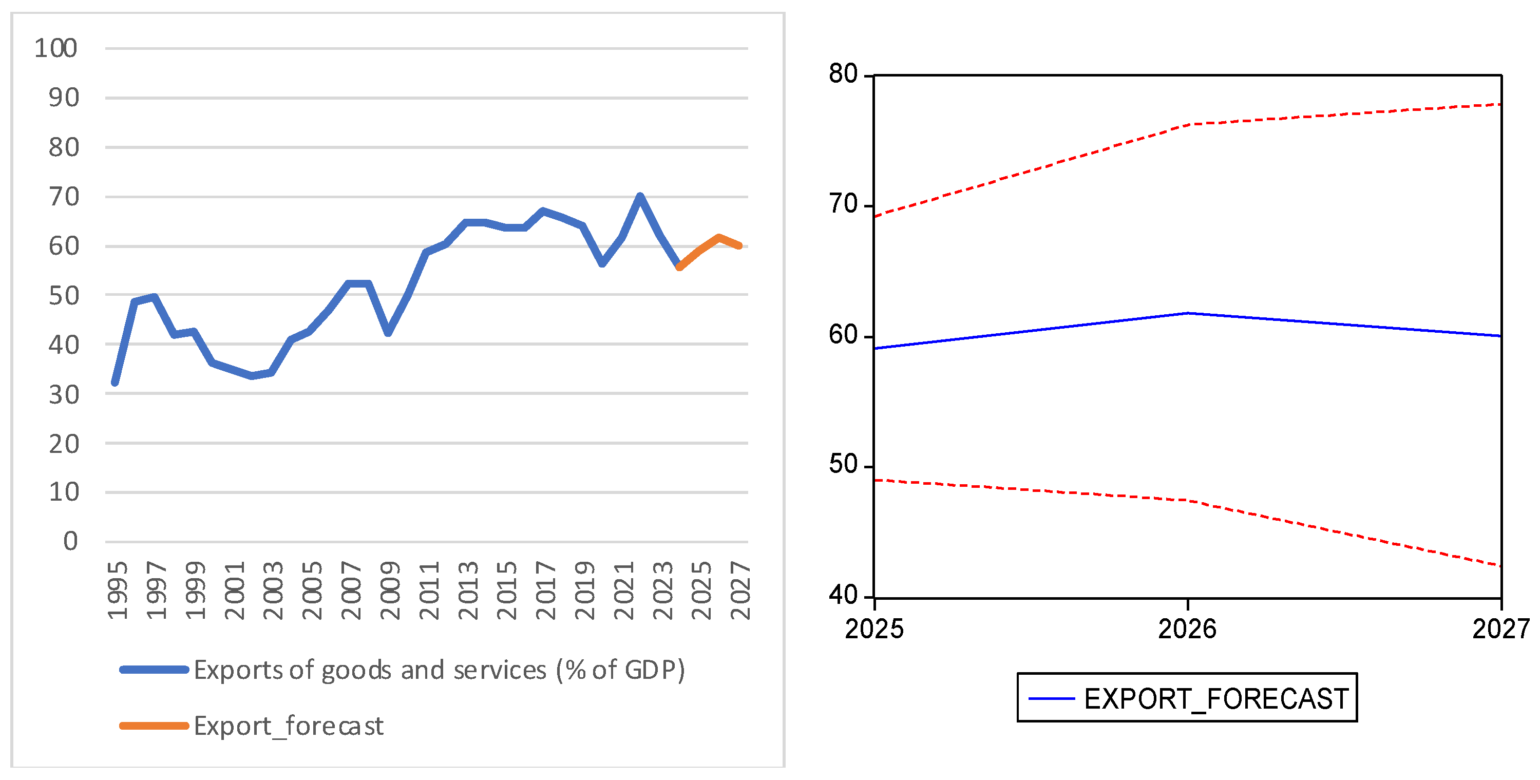
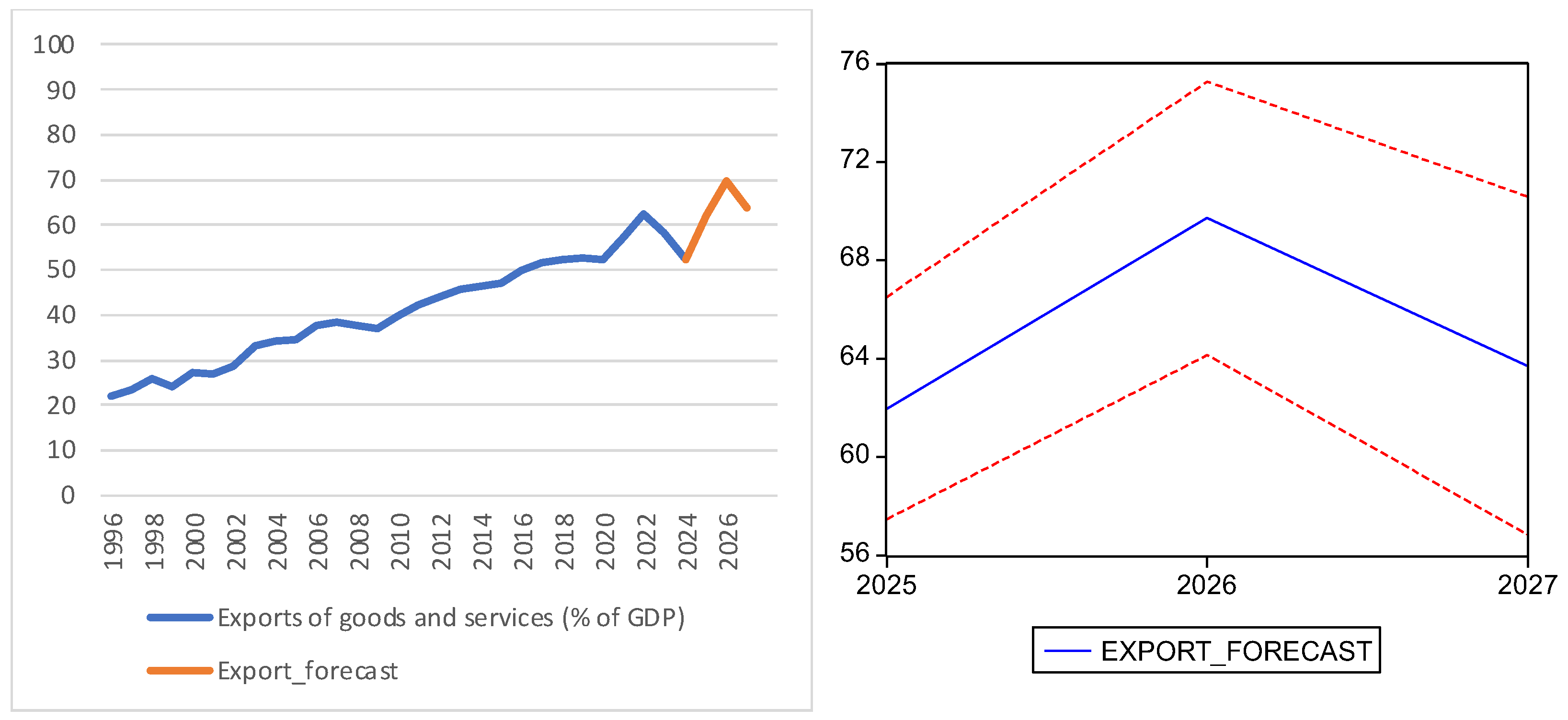
The optimal model is ARIMA(4,1,4) because it provides the best accuracy (MAPE = 12.1%, RMSE = 7.76) and has residual errors without autocorrelation and without heteroscedasticity, even if the AIC/SC are slightly higher than the others, but the difference is marginal. The estimate is: D(Export)_t = 0.7808 − 0.4746 × AR(4) + 0.8610 × MA(4) + ε_t.

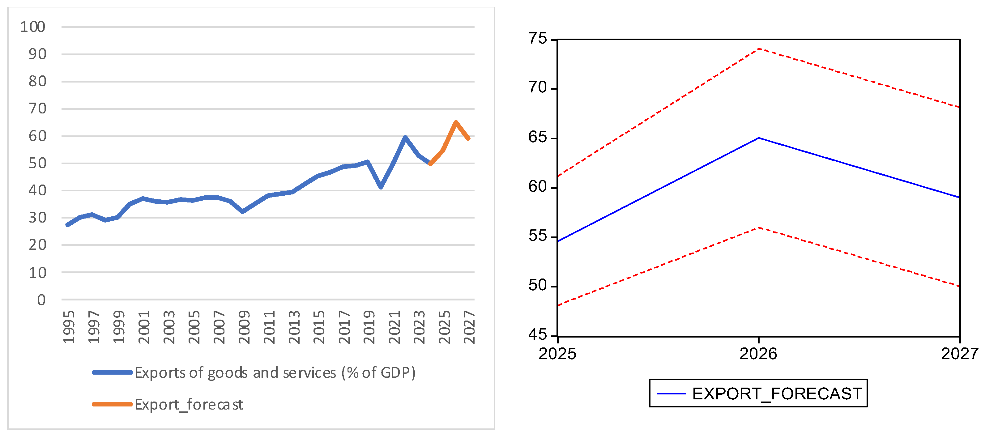
The forecast is given in

Table 8. Bulgaria export forecasts.

Bulgaria	Forecast 2025	Forecast 2026	Forecast 2027
ARIMA(4,1,4)	59.05%	61.79%	60.07%

Source: Authors’ contribution, based on data from the World Bank (Exports of Goods and Services).

and is graphically represented, with the confidence interval, in Figure 2. The ARIMA(4,1,4) model provides forecasts for EXPORT in the coming years, observing a trend of increasing the share of exports in GDP, which may indicate an improvement in Bulgaria’s economic competitiveness.

4.3.2. Croatia

Between 1995 and 2024, Croatia experienced a marked expansion in exports, reflecting both the country’s economic development and its progressive integration into global markets. During the early period of transition (1995–2013), export growth was gradual, shaped by structural reforms and pre-accession alignment with European Union standards. EU accession in 2013 represented a significant turning point, providing access to the European single market, eliminating trade barriers, and fostering regulatory harmonization. In the decade following accession, exports roughly doubled, contributing to an increase in GDP per capita from 50% to 75% of the EU average, highlighting the economic benefits of deeper European integration. In 2023, exports reached USD 44.67 billion, representing a 5.46% increase relative to the previous year (Trading Economics, n.d.-a).

Croatia’s export structure underscores the interplay between industrial capacity, foreign investment, and regional integration. Key sectors include pharmaceuticals (USD 697.1 million in 2022), chemicals (EUR 2.43 billion by October 2024), food and live animals (EUR 2.33 billion), and various manufactured goods (EUR 2.64 billion). Approximately 60% of exports are directed toward EU markets, reinforcing the centrality of European trade integration in shaping Croatia’s export performance. The expansion of export oriented FDI has contributed to this development by providing capital, technology, and managerial know-how, enabling domestic firms to participate more effectively in regional and global value chains.

Examining export share in GDP over 1995–2024 reveals a generally upward trend, punctuated by temporary contractions during the 2008–2009 financial crisis and the COVID-19 pandemic in 2020–2021. Exports averaged 39.85% of GDP, with a standard deviation of 7.99% and a coefficient of variation of 20.05%, indicating moderate variability around the mean. The Shapiro–Wilk test (p = 0.1) confirms approximate normality, supporting the robustness of the observed trend. Overall, Croatia’s export growth demonstrates the combined effect of structural reforms, EU integration, and foreign investment in fostering sustained economic expansion and integration into European and global markets. Using the correlogram, several ARIMA(p,1,q) models were tested, and comparisons between them are given in

Table 9. AIC, SC criteria, diagnostic tests and prediction errors for Croatia.

Model	AIC	SC	DW	B-G Test p-Value	ARCH Test p-Value	RMSE	MAPE
ARIMA(1,1,1)	5.387	5.529	1.74	0.16	0.81	4.51	9.12%
ARIMA(2,1,5)	5.264	5.408	2.36	0.43	0.02	3.56	6.53%
ARIMA(2,1,6)	5.123	5.267	2.54	0.26	0.37	4.28	8.22%
ARIMA(3,1,3)	5.715	5.860	2.02	0.0064	0.0108	3.84	7.47%

Source: Authors’ contribution, based on data from the World Bank (Exports of Goods and Services).

.

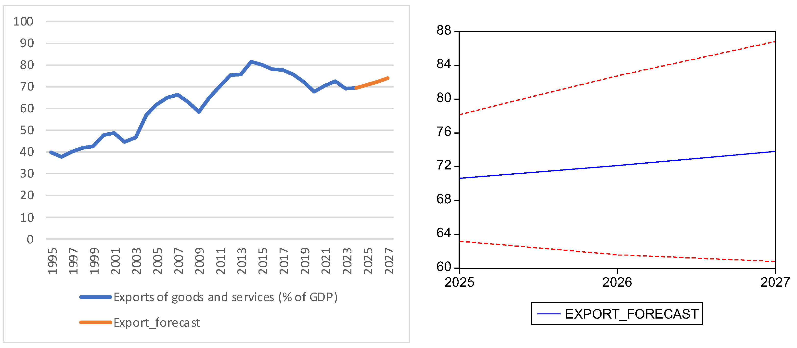
The optimal model for Croatia is chosen as ARIMA(2,1,6), because it has the lowest AIC/SC criteria, residuals without autocorrelation, constant variance (ARCH, p > 0.35), realistic forecast, without extreme oscillations. Although the ARIMA(2,1,5) model offers slightly higher accuracy (MAPE 6.5%), the ARCH test indicates the presence of heteroscedasticity (p ≈ 0.02). The ARIMA(2,1,6) model is preferred for its full statistical validity, absence of autocorrelation and stability of the residual variance. The estimation is D(Export)_t = 0.9372 − 0.4746 × AR(2) − 0.7928 × MA(6) + ε_t.

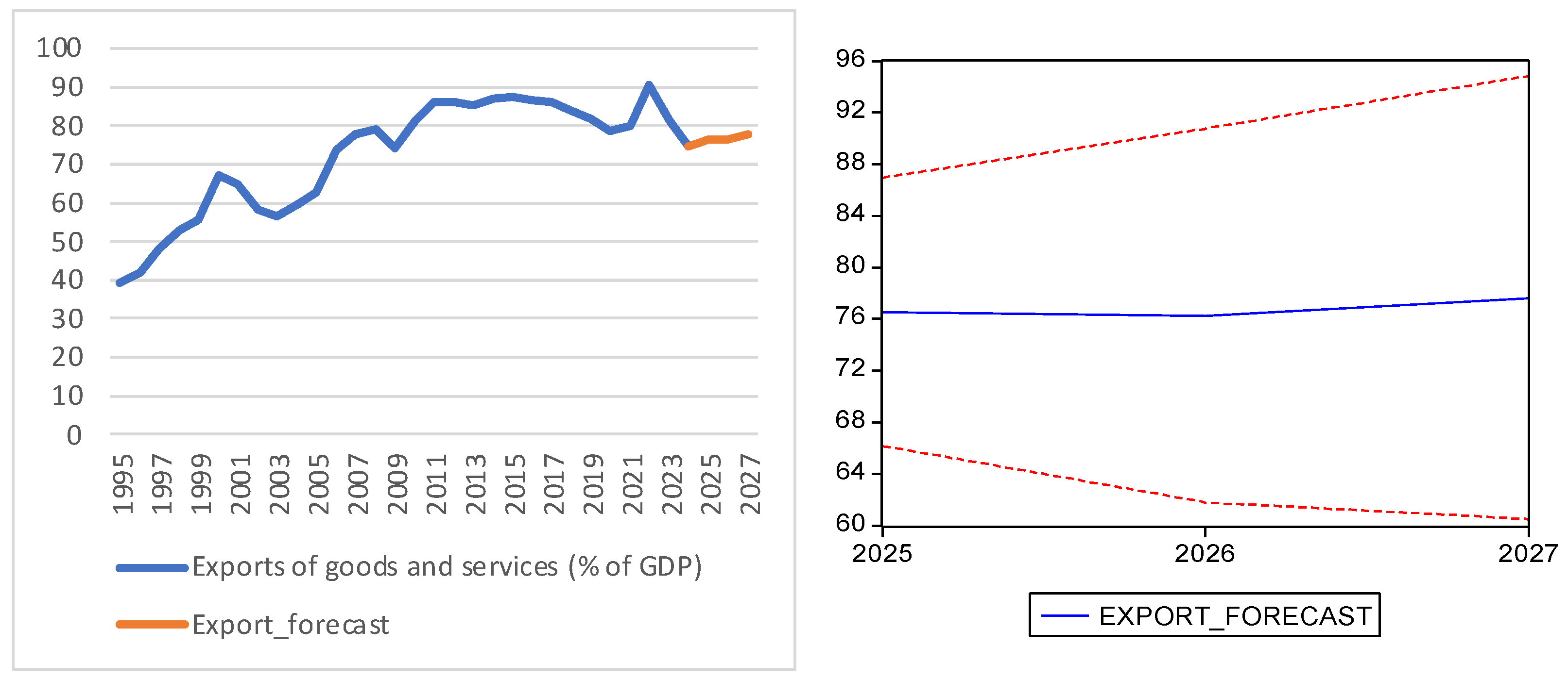
The forecast is found in

Table 10. Croatia export forecasts.

Croatia	Forecast 2025	Forecast 2026	Forecast 2027
ARIMA(2,1,6)	54.60%	65.02%	59.03%

Source: Authors’ contribution, based on data from the World Bank (Exports of Goods and Services).

and is graphically represented, with the confidence interval, in Figure 3.

4.3.3. Czech Republic

Following its separation from Slovakia in 1993, Czech Republic undertook a rapid transition to a market-oriented economy, attracting significant foreign direct investment and expanding its export sector. Geographic proximity and strong trade relations with Germany facilitated early export growth, a trend further reinforced by EU accession in 2004, which provided unrestricted access to European markets and harmonized regulatory standards.

Between 2005 and 2015, the Czech export sector experienced robust growth, driven primarily by the manufacturing industry and strategic infrastructure investments. The automotive industry emerged as a central pillar of the economy, with approximately one-third of exports destined for Germany, underscoring both the sector’s importance and the country’s dependence on key regional partners. Intra-regional trade within Central and Eastern Europe also expanded, reaching USD 237 billion by 2023, highlighting the significance of regional integration in shaping trade dynamics.

From 2016 to 2024, the Czech economy faced structural challenges linked to its reliance on foreign capital and the automotive sector. While GDP per capita reached 91% of the EU average in 2022, the limitations of a growth model based on low-cost labor and foreign investment became increasingly apparent. In response, economic policy and corporate strategy shifted toward innovation and the development of higher value-added sectors, reinforcing the technological sophistication and competitiveness of exports. Throughout this period, Czech exports remained concentrated in machinery and transport equipment, reflecting the enduring strength of the manufacturing sector, with Germany continuing to absorb roughly one-third of total exports, complemented by other EU and Central and Eastern European markets.

Over the entire period, exports averaged 62% of GDP, with a standard deviation of 13.84% and a coefficient of variation of 22.32%, indicating moderate fluctuations around a representative mean. The Shapiro–Wilk test (p = 0.013) reveals deviations from normality, suggesting asymmetric fluctuations in export performance. The historical trajectory illustrates how the combination of FDI, regional integration, and structural innovation has underpinned the Czech Republic’s export growth and economic modernization, providing a foundation for sustainable medium- and long-term development. Using the D(Export) correlogram, several ARIMA models resulted, with the main indicators in

Table 11. AIC, SC criteria, diagnostic tests and prediction errors for Czech Republic.

Model	AIC	SC	DW	B-G Test p-Value	ARCH Test p-Value	RMSE	MAPE
ARIMA(3,1,3)	5.4038	5.549	1.69	0.23	0.92	22.7	29.25
ARIMA(4,1,4)	5.4701	5.616	1.53	0.65	0.92	10.52	12.28
ARIMA(5,1,6)	5.3770	5.524	1.63	0.72	0.21	14.94	19.05

Source: Authors’ contribution, based on data from the World Bank (Exports of Goods and Services).

.

The recommended model for the Czech Republic is ARIMA(4,1,4) because RMSE and MAPE have the lowest values, resulting in the best forecast accuracy. The B-G and ARCH tests confirm the lack of correlation of residuals and heteroscedasticity. Even though the AIC/SC are slightly higher than the other models, the difference is unsignificant and marginal. The estimate is D(Export)_t = 1.1691 − 0.6269 × AR(4) + 0.9248 × MA(4) + ε_t.

The forecast can be found in

Table 12. Czech Republic export forecasts.

Czech Republic	Forecast 2025	Forecast 2026	Forecast 2027
ARIMA(4,1,4)	70.65%	72.12%	73.77%

Source: Authors’ contribution, based on data from the World Bank (Exports of Goods and Services).

and is graphically represented, with the confidence interval, in Figure 4.

4.3.4. Hungary

Between 1995 and 2024, Hungary experienced a sustained increase in exports, reflecting the country’s diversified economy and strong manufacturing base. Total exports grew from approximately EUR 1.43 billion in January 1999 to a historical peak of EUR 14.31 billion in March 2023. Key export sectors include vehicles and transport equipment, electrical machinery and equipment, pharmaceuticals, chemicals, and food and beverages (Eulerpool Research Systems, n.d.). Germany has consistently been Hungary’s principal trading partner, supported by close economic ties and substantial German investment, while Austria, Romania, China, and Italy also represent significant markets.

Over the analyzed period, exports averaged 72.21% of GDP, with a standard deviation of 14.78% and a coefficient of variation of 20.47%, indicating moderate fluctuations around the mean. The Shapiro–Wilk test (p = 0.006) suggests deviations from normality, reflecting asymmetric variations in export performance. Despite occasional declines, such as the 0.8% contraction in 2023 due to global and regional economic challenges, Hungary’s export sector has demonstrated resilience, diversification, and a growing integration into international markets. Using the information from the D(Export) correlogram, several ARIMA models were validated, according to

Table 13. AIC, SC criteria, diagnostic tests and prediction errors for Hungary.

Model	AIC	SC	DW	B-G Test p-Value	ARCH Test p-Value	RMSE	MAPE
ARIMA(1,1,1)	6.1661	6.309	1.68	0.31	0.49	23.25	26.98
ARIMA(2,1,2)	6.1085	6.252	1.69	0.14	0.43	12.23	13.36
ARIMA(6,1,7)	5.5875	5.736	2.02	0.13	0.77	31.53	32.82

Source: Authors’ contribution, based on data from the World Bank (Exports of Goods and Services).

.

The optimal model for Hungary is chosen as ARIMA(2,1,2) because the residuals are uncorrelated; it is homoscedastic and it has the lowest RMSE and MAPE values among the tested models, even if the AIC/SC are slightly higher. The model has a balanced prediction performance. The estimation is D(Export)_t = 0.1753 + 0.6914 × AR(2) − 0.8901 × MA(2) + ε_t.

The forecast is found in

Table 14. Hungary export forecasts.

Hungary	Forecast 2025	Forecast 2026	Forecast 2027
ARIMA(2,1,2)	76.54%	76.27%	77.62%

Source: Authors’ contribution, based on data from the World Bank (Exports of Goods and Services).

and is graphically represented, with the confidence interval, in Figure 5. The ARIMA model suggests a moderate growth trend in the coming years and suggests a stabilization of exports at a high level.

4.3.5. Poland

Between 1995 and 2024, Poland experienced a sustained and significant expansion of its exports, reflecting the country’s increasing integration into European and global markets and the gradual modernization of its economy. Exports grew from approximately USD 22.89 billion in 1995 to USD 31.6 billion in 2000, with EU accession in 2004 accelerating trade growth by facilitating access to European markets and enhancing economic convergence. By 2023, exports had increased sixfold compared to 2010 levels, reaching USD 469.01 billion, and contributing to Poland achieving 80% of the EU average in GDP per capita adjusted for purchasing power. These developments positioned Poland among the world’s top 20 markets, accounting for approximately 1% of global GDP and 1.4% of world exports (Macrotrends, n.d.).

In 2023, the main export destinations were Germany (27%), the Czech Republic (6.27%), France (6.16%), the United Kingdom (4.94%), and Italy (4.57%). Key export categories included machinery and mechanical equipment (13.9%), electrical equipment (12.3%), and vehicles and components (10.7%) (Trading Economics, n.d.-b).

Analysis of export share in GDP over the 1995–2024 period indicates an average of 40.24%, with a standard deviation of 11.83% and a coefficient of variation of 29.41%, reflecting substantial volatility relative to the mean. The series exhibited a minimum of 21.98% in 1996 and a maximum of 62.35% in 2022. The Shapiro–Wilk test (p = 0.195) suggests that the data are approximately normally distributed. Overall, Poland’s export performance illustrates the adaptability, competitiveness, and structural transformation of its economy over the past three decades, underpinned by EU integration, industrial diversification, and a sustained expansion in international trade. From the analysis of the D(Export) correlogram, several ARIMA models were verified with the indicators presented in

Table 15. AIC, SC criteria, diagnostic tests and prediction errors for Poland.

Model	AIC	SC	DW	B-G Test p-Value	ARCH Test p-Value	RMSE	MAPE
ARIMA(2,1,1)	4.1729	4.3169	1.63	0.33	0.79	2.5125	4.28
ARIMA(2,1,4)	4.1201	4.2641	2.04	0.21	0.48	3.0957	6.25
ARIMA(2,1,6)	3.8104	3.9544	2.24	0.07	0.12	7.4565	13.13

Source: Authors’ contribution, based on data from the World Bank (Exports of Goods and Services).

.

The most suitable model for Poland was chosen to be ARIMA(2,1,1) as it presented the lowest RMSE/MAPE values, without residual correlation and constant variance; even if AIC/SC had slightly higher values, these were marginal. The estimate is D(Export)_t = 1.3663 − 0.8901 × AR(2) − 0.9354 × MA(1) + ε_t.

The forecast is found in

Table 16. Poland export forecasts.

Poland	Forecast 2025	Forecast 2026	Forecast 2027
ARIMA(2,1,1)	61.97%	69.70%	63.70%

Source: Authors’ contribution, based on data from the World Bank (Exports of Goods and Services).

and is graphically represented, with the confidence interval, in Figure 6. The forecast indicates an increasing trend in Polish exports, then followed by decreasing.

4.3.6. Romania

Between 1995 and 2024, Romania’s exports exhibited substantial growth in both total value and sectoral diversification, reflecting the country’s structural economic transformation and deeper integration into European markets. Total exports increased from an average of USD 5.2 billion in 2003 to USD 100.6 billion in 2023, with Germany, Italy, and Hungary emerging as the main trading partners, accounting for 19%, 10%, and 7% of total exports, respectively (World’s Top Exports, n.d.-a).

Romania’s export portfolio became increasingly diversified, encompassing the automotive industry, industrial products and equipment, and agricultural and food products. Over the 1995–2024 period, exports averaged 32.03% of GDP, with a standard deviation of 7.7% and a coefficient of variation of 24.06%, indicating that the mean provides a representative measure despite moderate fluctuations. The minimum and maximum values were 24.58% (2000) and 43.36% (2022), respectively. The Shapiro–Wilk test (p = 0.001) indicates deviations from normality, suggesting asymmetrical variations in the data.

Temporally, exports displayed a clear upward trend between 2001 and 2019, which intensified after 2010, coinciding with post-crisis recovery and the consolidation of EU integration benefits following Romania’s accession in 2007. This trajectory was briefly interrupted in 2020 due to the COVID-19 pandemic but resumed in subsequent years, although a slight decline has been observed in the most recent two-year period. The evolution of Romania’s exports highlights the combined effect of EU integration, sectoral diversification, and structural economic reforms in enhancing international competitiveness. The analysis of the D(Export) correlogram suggested several possible ARIMA models, with the indicators presented in

Table 17. AIC, SC criteria, diagnostic tests and prediction errors for Romania.

Model	AIC	SC	DW	B-G Test p-Value	ARCH Test p-Value	RMSE	MAPE
ARIMA(1,1,1)	4.7393	4.8820	1.96	0.95	0.59	7.244	17.89
ARIMA(2,1,2)	4.7438	4.8878	1.64	0.30	0.46	8.265	25.56
ARIMA(2,1,3)	4.7229	4.8668	1.67	0.97	0.33	5.301	16.44

Source: Authors’ contribution, based on data from the World Bank (Exports of Goods and Services).

.

The most suitable model for Romania was chosen to be ARIMA(2,1,3), as it had the lowest values of RMSE/MAPE and AIC/SC criteria. The estimation is D(Export)_t = 0.5442 − 0.4771 × AR(2) + 0.9009 × MA(3) + ε_t.

The forecast is found in

Table 18. Romania export forecasts.

Romania	Forecast 2025	Forecast 2026	Forecast 2027
ARIMA(2,1,3)	40.48%	43.50%	37.68%

Source: Authors’ contribution, based on data from the World Bank (Exports of Goods and Services).

and is graphically represented, with the confidence interval, in Figure 7.

4.3.7. Slovakia

Between 1995 and 2024, Slovakia experienced a significant expansion of its exports, reflecting the country’s economic transition, industrial development, and integration into European economic structures. Total exports increased from USD 32.6 billion in 2003 to USD 117.1 billion in 2023, representing a growth of approximately 259%. The export portfolio has diversified over this period, with key sectors including the automotive industry, electrical machinery and equipment, metallurgical products, chemicals, and pharmaceuticals. Slovakia’s primary trading partners in 2023 were Germany, the Czech Republic, Poland, and Hungary, reflecting strong regional and EU-oriented trade linkages (World’s Top Exports, n.d.-b).

Export share in GDP exhibited a generally consistent upward trend from 1997 to 2024, interrupted by temporary declines during the global financial crisis (2008–2009) and the COVID-19 pandemic. The average export share over the analyzed period was 76.12%, with a standard deviation of 17.15% and a coefficient of variation of 22.53%, indicating moderate variability around the mean. The Shapiro–Wilk test (p = 0.004) suggests deviations from normality, reflecting asymmetric fluctuations in export performance. Overall, Slovakia’s export evolution underscores the role of foreign investment, sectoral diversification, and EU integration in sustaining trade growth and economic modernization. Using the D(Export) correlogram, several possible ARIMA models were analyzed, with the indicators given in

Table 19. AIC, SC criteria, diagnostic tests and prediction errors for Slovakia.

Model	AIC	SC	DW	B-G Test p-Value	ARCH Test p-Value	RMSE	MAPE
ARIMA(2,1,6)	5.998	6.142	1.87	0.47	0.31	16.25	17.38
ARIMA(2,1,7)	6.085	6.229	1.70	0.44	0.29	21.61	22.88
ARIMA(2,1,8)	5.930	6.074	1.73	0.60	0.50	13.34	14.35
ARIMA(2,1,9)	5.759	5.903	1.66	0.65	0.07	20.51	21.80
ARIMA(2,1,10)	5.791	5.935	2.06	0.76	0.65	17.01	18.20

Source: Authors’ contribution, based on data from the World Bank (Exports of Goods and Services).

.

Based on the analysis of the evaluation indicators, the most suitable model for Slovakia among the validated specifications is ARIMA(2,1,8), as it yields the lowest RMSE and MAPE values, indicating the best forecasting accuracy. Although the corresponding AIC and SC values are slightly higher, the differences are marginal and do not compromise the model’s overall performance. The estimated equation is: D(Export)_t = 1.0787 − 0.4951 × AR(2) − 0.8671 × MA(8) + ε_t.

The forecast is found in

Table 20. Slovakia export forecasts.

Slovakia	Forecast 2025	Forecast 2026	Forecast 2027
ARIMA(2,1,8)	93.91%	96.61%	94.90%

Source: Authors’ contribution, based on data from the World Bank (Exports of Goods and Services).

and is graphically represented, with the confidence interval, in Figure 8.

The empirical results yield several important implications for economic policy and applied trade analysis in Central and Eastern Europe. First, the identification of persistent upward trends in export intensity across all countries confirms the long-term effectiveness of EU integration and trade liberalization as drivers of export-led growth. However, the marked heterogeneity in export dependence and volatility suggests that highly open economies—such as Slovakia, Hungary, and the Czech Republic—remain more exposed to external demand shocks, particularly in cyclical manufacturing sectors. This finding underscores the importance of export diversification and value-chain upgrading as mechanisms for enhancing resilience.

Second, the Granger causality results reveal that foreign direct investment contributes to export growth only in a subset of countries and often with significant time lags. This implies that FDI inflows alone are insufficient to generate immediate export expansion; instead, complementary factors such as absorptive capacity, infrastructure quality, and institutional effectiveness are critical for translating investment into export competitiveness. From a policy perspective, this highlights the need for targeted industrial and innovation policies that facilitate technology diffusion and firm-level integration into global value chains.

Finally, the robustness of the ARIMA-based forecasts indicates that, despite recent shocks—including the global financial crisis, the COVID-19 pandemic, and geopolitical disruptions—export dynamics in CEE economies exhibit a degree of structural stability. This supports the use of classical time-series models as reliable tools for short-term export forecasting and policy planning, particularly when the objective is to project aggregate export dependence rather than sector-specific performance.

5. Discussion and Conclusions

The comparative analysis of export dynamics in Central and Eastern European (countries over the period 1995–2024) reveals a consistent process of growth and structural transformation, driven by the transition to a market economy, trade liberalization, and European integration. The results confirm the theoretical assumption that economic integration and foreign direct are key factors in strengthening external performance and promoting convergence toward the standards of the more advanced economies of the European Union.

All analyzed economies display a clear upward trend in exports as a share of GDP, reflecting the consolidation of industrial processes, capital accumulation, and the expansion of productive capacity. The stationarity tests (ADF) indicate that the series are non-stationary at level but become stable after first differencing, suggesting the existence of long-term trends. These findings point to a structural and predictable evolution of exports, shaped by enduring macroeconomic and institutional factors.

Overall, the CEE countries share common characteristics regarding their export orientation toward European markets, yet they differ in terms of their degree of economic openness and integration into continental value chains. The Czech Republic, Slovakia, and Hungary stand out as highly open economies, with exports accounting for over 70–90% of GDP, deeply integrated into the European automotive and electronics industries. Bulgaria and Croatia exhibit a medium level of openness, with exports representing 40–60% of GDP and a mixed structure combining industry, services, and tourism. Poland and Romania, with larger domestic markets, display lower export shares of 30–45% but maintain steady and more diversified growth, suggesting greater resilience to external shocks.

The Mann–Whitney tests indicate significant differences between most pairs of countries, confirming the existence of statistically distinct populations. These variations can be explained by differences in national policies for attracting foreign direct investment, the level of economic infrastructure, the degree of industrialization, and overall macroeconomic stability.

The results of the Granger causality tests provide a nuanced view of the interdependence between FDI and exports. For Romania, the Czech Republic, and Croatia, the analysis confirms a unidirectional or bidirectional causality between FDI and export performance, supporting the hypothesis that investment inflows stimulate the development of export capacity—after a certain time lag—through technology transfer and managerial know-how. In contrast, for Hungary, Poland, Bulgaria, and Slovakia, the relationship is not statistically significant in the short term, suggesting either a longer adjustment period for these effects to materialize or that a portion of foreign investment has been directed toward non-export-oriented sectors such as services, energy, or infrastructure.

The validated ARIMA models for each economy indicate a general trend of moderate growth and stabilization in the share of exports in GDP over the 2025–2027 period. The highest levels are forecast for Slovakia (approximately 95%), Hungary (around 77%), and the Czech Republic (about 74%), confirming their profile as export-oriented manufacturing economies. Poland and Bulgaria show gradual increases, reflecting the strengthening of industrial competitiveness. Romania and Croatia follow an upward trajectory until 2026, followed by a slight adjustment, possibly associated with cyclical effects and structural constraints. Overall, the forecasts suggest a continued process of regional convergence, albeit at a slower pace, driven by structural limitations and a high dependence on European external demand.

In addition, these findings confirm a common upward trend in export performance across CEE markets between 1995 and 2024 (RQ1), reflecting the cumulative effects of market liberalization, EU integration, and sustained inflows of foreign direct investment. Despite initial structural disparities, all countries have experienced a gradual increase in the share of exports in GDP, with statistical tests indicating stable long-term growth trends. The Granger causality analysis further demonstrates that FDI has been a significant driver of export performance (RQ2), particularly in Romania, the Czech Republic, and Croatia, where bidirectional or unidirectional causal relationships were identified. This finding supports the view that foreign investment has acted as a conduit for technology transfer and productivity gains, thereby strengthening export competitiveness. At the same time, significant cross-country differences persist (RQ3), as revealed by the Mann–Whitney tests, suggesting the coexistence of distinct structural and institutional trajectories driven by each country’s integration depth, industrial capacity, and investment orientation.

The analysis also reveals important nuances in the relationship between economic openness and export stability (RQ4). Highly open markets such as Slovakia, Hungary, and the Czech Republic exhibit strong export dependence but greater exposure to external shocks, whereas larger domestic markets like Poland and Romania display more moderate yet stable export shares due to the cushioning effect of internal demand. The ARIMA-based forecasts (RQ5) confirm a continued, moderate rise in exports through 2025–2027, with the highest projected levels in Slovakia, Hungary, and the Czech Republic, and more gradual increases in Poland, Bulgaria, and Romania. Finally, the evidence indicates that export growth contributes to economic convergence within the EU (RQ6), although at uneven rates: Central European markets are advancing faster due to higher industrial sophistication and value-chain integration, while Southeastern members continue to face structural and infrastructural constraints that slow their convergence pace.

The results of this study carry important policy implications for trade and industrial strategy in Central and Eastern Europe. The forecasted trends indicate that export growth in the region remains closely tied to integration within EU value chains and to the inflow of foreign direct investment, which continues to act as a catalyst for productivity upgrading and technological diffusion. Policymakers should therefore prioritize measures that sustain these linkages—such as strengthening innovation capacity, promoting technology-intensive sectors, and improving institutional efficiency—to ensure that future export expansion contributes to long-term competitiveness rather than dependence on low-value production. Moreover, the observed differences in export trajectories across CEE markets highlight the need for tailored industrial policies that account for each country’s structural position within the regional supply network.

Beyond its empirical findings, this research also adds a conceptual contribution by linking export forecasting to broader debates on regional convergence and sustainable development. The results suggest that continued export dynamism is essential for narrowing income gaps with Western Europe, but that diversification and resilience are equally critical for achieving sustainable growth. Incorporating trade forecasting into policy planning can help governments anticipate external shocks, evaluate the potential impact of EU trade policies, and design strategies consistent with the green and digital transitions outlined in the EU’s sustainability agenda. Thus, the study provides a forward-looking analytical tool for both scholars and policymakers seeking to align export performance with the long-term objectives of competitiveness, convergence, and sustainable development in the CEE region.

The research results provide a useful basis for redefining the industrial and trade strategies of Central and Eastern European countries. The projected growth in exports can support the reorientation of public policies toward strengthening high value-added industrial sectors, particularly in technology and energy industries; encouraging public–private partnerships in infrastructure, innovation, and technological education; diversifying export markets beyond the European Union through expansion into Asia, the Middle East, and North Africa; and reducing vulnerability to external shocks by developing local industries and promoting regional supply chains.

At the regional level, export growth has the potential to accelerate economic convergence, but only if it is accompanied by coordinated policies on innovation, infrastructure, and human capital. Without these components, dependence on traditional industrial exports may perpetuate an “incomplete” convergence, driven more by low costs than by innovation and productivity. From an academic perspective, the study contributes through an integrated analysis of the relationship between FDI and exports using robust methods such as Granger causality and ARIMA modeling; a longitudinal comparative approach covering seven CEE economies over an extended period (1995–2024); and applied econometric forecasts that can support data-driven policy formulation and the assessment of European integration’s impact on trade performance. Thus, this research provides a valuable strategic reference tool for policymakers, the business community, and regional institutions, while also contributing to the academic literature on economic convergence and export-led growth models in post-transition Europe.

However, this paper faces several methodological and empirical limitations. The use of aggregated data (as a percentage of GDP) does not capture intra-sectoral variations; the results may be affected by methodological changes in national statistics and by exceptional events such as crises, pandemics, or regional conflicts; and the post-2022 period is influenced by geopolitical and economic uncertainties—including the war in Ukraine, inflation, and energy market volatility—which may cause deviations from the statistically modeled trends.

A limitation of the present study is the use of aggregated export data expressed as a percentage of GDP, which does not capture intra-industry and sectoral heterogeneity. While this measure is suitable for cross-country comparability and long-term macroeconomic analysis, it may obscure substantial differences in export intensity, volatility, and shock sensitivity across industries. In particular, export volatility at the aggregate level may be driven by a limited number of highly cyclical sectors, such as manufacturing industries deeply integrated into global value chains, while other sectors exhibit more stable export patterns. Similarly, the absence of Granger causality between FDI and exports in some countries may reflect the concentration of foreign investment in services or domestic-market-oriented activities, whose export effects are not fully captured in aggregate measures. Consequently, the findings should be interpreted as reflecting overall export dynamics rather than sector-specific export behavior. From a policy perspective, this suggests that export promotion and FDI attraction strategies should be increasingly tailored to sectoral characteristics, with a focus on diversification, upgrading toward higher value-added activities, and reducing excessive dependence on a narrow set of export-oriented industries. Future research could extend the present analysis by employing disaggregated, sector-level data to better capture these intra-industry dynamics.

Also, the ARIMA-based forecasts for the post-2022 period should be interpreted with caution, as they are generated under the assumption that historical patterns and relationships persist over time. While the models capture long-run trends and cyclical dynamics in export performance, they do not explicitly account for major external shocks or structural breaks. In this context, recent geopolitical tensions, particularly the war in Ukraine, as well as the energy crisis affecting European economies, may alter trade flows, production costs, and export competitiveness in ways that deviate from historical dynamics. Highly open economies with strong energy import dependence may experience greater volatility than projected by the baseline ARIMA forecasts, whereas countries with larger domestic markets may exhibit a stronger buffering effect.

Therefore, the forecast results should be viewed as baseline scenarios rather than unconditional predictions. Future research could incorporate structural break tests, regime-switching models, or multivariate forecasting frameworks to explicitly capture the impact of external shocks on export dynamics.

To strengthen the results and broaden their interpretation, future research could employ multivariate models (such as ARIMAX, VAR, or VECM) to capture the dynamic interdependencies among exports, FDI, GDP, exchange rates, and other macroeconomic factors; analyze the sectoral dimension of exports to identify the industries with the highest multiplier effects; and incorporate institutional and governance variables that influence external competitiveness.

References

1. Balassa, B. (1965). Trade liberalization and revealed comparative advantage. The Manchester School of Economic and Social Studies, 33, 99–123. [Google Scholar] [CrossRef]
2. Bierut, B., & Kuziemska-Pawlak, K. (2016). Competitiveness and export performance of CEE countries. NBP Working Papers, Article 248. Available online: https://ideas.repec.org//p/nbp/nbpmis/248.html (accessed on 15 September 2025).
3. Borys, M. M., Polgár, É. K., & Zlate, A. (2008). Real convergence and the determinants of growth in EU candidate and potential candidate countries: A panel data approach. ECB Occasional Paper Series, 86. ECB. [Google Scholar]
4. Box, G. E. P., Jenkins, G. M., Reinsel, G. C., & Ljung, G. M. (2016). Time series analysis: Forecasting and control (5th ed., Vol. 37). Wiley. Available online: https://onlinelibrary.wiley.com/doi/abs/10.1111/jtsa.12194 (accessed on 15 September 2025).
5. Breusch, T. S. (1978). Testing for autocorrelation in dynamic linear models. Australian Economic Papers, 17(31), 334–355. [Google Scholar] [CrossRef]
6. Bussière, M., Fidrmuc, J., & Schnatz, B. (2005). Trade integration of central and eastern European countries. ECB Working Paper Series, 545. ECB. [Google Scholar]
7. Cieślik, A., Michałek, J. J., & Mycielski, J. (2012). Measuring the trade effects of the euro in Central and Eastern Europe. The Journal of International Trade & Economic Development, 21(1), 25–49. [Google Scholar] [CrossRef]
8. Dai, C. (2023). A method of forecasting trade export volume based on back-propagation neural network. Neural Computing and Applications, 35(12), 8775–8784. [Google Scholar] [CrossRef]
9. Davidescu, A. A., Popovici, O. C., & Strat, V. A. (2022). An empirical analysis using panel data gravity models and scenario forecast simulations for the Romanian exports in the context of COVID-19. Economic Research-Ekonomska Istraživanja, 35(1), 480–510. [Google Scholar] [CrossRef]
10. Deij, S., Madsen, J. B., & Puzzello, L. (2018). Does trade matter for growth when the geographical instruments are randomly generated? Geneva Trade and Development Workshop. Available online: https://www.wto.org/english/res_e/reser_e/gtdw_e/wkshop18_e/puzzello_e.pdf#:~:text=In%20their%20seminal%20paper%20Frankel,sum%20up%20predicted%20bilateral%20shares (accessed on 15 September 2025).
11. Dickey, D. A., & Fuller, W. A. (1979). Distribution of the estimators for autoregressive time series with a unit root. Journal of the American Statistical Association, 74(366a), 427–431. [Google Scholar] [CrossRef] [PubMed]
12. Durbin, J., & Watson, G. S. (1950). Testing for serial correlation in least squares regression. I. Biometrika, 37(3–4), 409–428. [Google Scholar] [CrossRef] [PubMed]
13. Engle, R. F. (1982). Autoregressive conditional heteroscedasticity with estimates of the variance of United Kingdom inflation. Econometrica, 50(4), 987–1007. [Google Scholar] [CrossRef]
14. Eulerpool Research Systems. (n.d.). Hungarian exports. Available online: https://eulerpool.com/ro/macro/ungaria/exports (accessed on 19 October 2025).
15. Fertő, I. (2007). The dynamics of trade in central and eastern European countries. Managing Global Transitions, 5(1), 5–23. [Google Scholar]
16. Frankel, J. A., & Romer, D. H. (1999). Does trade cause growth? American Economic Review, 89(3), 379–399. [Google Scholar] [CrossRef]
17. Gábor Márk Pellényi. (2020). The role of Central & Eastern Europe in global value chains: Evidence from occupation level employment data (ECONOMIC BRIEF No. 062, p. 20). European Commission (EC). [Google Scholar] [CrossRef]
18. Gilbert, J., & Muchová, E. (2018). Export competitiveness of Central and Eastern Europe since the enlargement of the EU. International Review of Economics & Finance, 55, 78–85. [Google Scholar] [CrossRef]
19. Giucă, A. D., Berevoianu, R., & Ilie, D. M. (2024). The dynamics of trade in vegetables in Romania. Proceedings of the International Conference on Business Excellence, 18(1), 1563–1570. [Google Scholar] [CrossRef]
20. Godfrey, L. G. (1978). Testing against general autoregressive and moving average error models when the regressors include lagged dependent variables. Econometrica, 46(6), 1293–1301. [Google Scholar] [CrossRef]
21. Grossman, G. M., & Helpman, E. (1991). Trade, knowledge spillovers, and growth. European Economic Review, 35(2), 517–526. [Google Scholar] [CrossRef]
22. Istudor, N., Constantin, M., Ignat, R., Chirpuci, B.-C., & Petrescu, I.-E. (2022). The complexity of agricultural competitiveness: Going beyond the Balassa index. Journal of Competitiveness, 14(4), 61–77. [Google Scholar] [CrossRef]
23. Jambor, A., & Gorton, M. (2025). Twenty years of EU accession: Learning lessons from central and eastern European agriculture and rural areas. Agricultural and Food Economics, 13(1), 1. [Google Scholar] [CrossRef]
24. Jirasavetakul, L.-B. F., & Rahman, J. (2018). Foreign direct investment in new member state of the EU and western Balkans: Taking stock and assessing prospects. IMF Working Papers, 18. Available online: https://www.imf.org/en/Publications/WP/Issues/2018/08/21/Foreign-Direct-Investment-in-New-Member-State-of-the-EU-and-Western-Balkans-Taking-Stock-and-46152 (accessed on 15 September 2025).
25. Karabay, G., Kilic, M. B., Saricoban, K., & Günaydin, G. K. (2023). Forecasting of Turkey’s apparel exports using artificial neural networkautoregressive models. Industria Textila, 74(02), 143–153. [Google Scholar] [CrossRef]
26. Kos-Labedowicz, J., & Talar, S. (2024). Trade resilience of central and eastern European countries to the shock caused by the Russia–Ukraine war. Forum Scientiae Oeconomia, 12(4), 4. [Google Scholar] [CrossRef]
27. Krugman, P. R. (1980). Scale economies, product differentiation, and the pattern of trade. The American Economic Review, 70(5), 950–959. [Google Scholar]
28. Kuc-Czarnecka, M., Saltelli, A., Olczyk, M., & Reinert, E. (2021). The opening of central and eastern European countries to free trade: A critical assessment. Structural Change and Economic Dynamics, 58, 23–34. [Google Scholar] [CrossRef]
29. Lehmann, R. (2021). Forecasting exports across Europe: What are the superior survey indicators? Empirical Economics, 60(5), 2429–2453. [Google Scholar] [CrossRef]
30. Lima, S., Gonçalves, A. M., & Costa, M. (2024). Predictive accuracy of time series models applied to economic data: The European countries retail trade. Journal of Applied Statistics, 51(9), 1818–1841. [Google Scholar] [CrossRef] [PubMed]
31. Lucas, R. E. (1988). On the mechanics of economic development. Journal of Monetary Economics, 22(1), 3–42. [Google Scholar] [CrossRef]
32. Macrotrends. (n.d.). Poland exports | historical chart & data. Available online: https://www.macrotrends.net/global-metrics/countries/pol/poland/exports (accessed on 19 October 2025).
33. Mahmoud Sayed Agbo, H. (2023). Forecasting agricultural price volatility of some export crops in Egypt using ARIMA/GARCH model. Review of Economics and Political Science, 8(2), 123–133. [Google Scholar] [CrossRef]
34. Mann, H. B., & Whitney, D. R. (1947). On a test of whether one of two random variables is stochastically larger than the other. The Annals of Mathematical Statistics, 18(1), 50–60. [Google Scholar] [CrossRef]
35. Melitz, M. J. (2003). The impact of trade on intra-industry reallocations and aggregate industry productivity. Econometrica, 71(6), 1695–1725. [Google Scholar] [CrossRef]
36. Petrova, B., & Sznajder Lee, A. (2024). Integrating with the global economy: The evolution of the export profiles of the European Union’s eastern periphery (2000–2021). Europe-Asia Studies, 76(5), 696–719. [Google Scholar] [CrossRef]
37. Pilinkiene, V. (2016). Trade openness, economic growth and competitiveness. The case of the central and eastern European countries. Engineering Economics, 27(2), 2. [Google Scholar] [CrossRef]
38. Popescu, L., Găman, M., Mihai, L.-S., Mihai, M., & Drăgan, C. O. (2025). Study on the evolution and forecast of agricultural raw material exports in emerging economies in Central and Eastern Europe using statistical methods. Agriculture, 15(17), 1811. [Google Scholar] [CrossRef]
39. Shapiro, S. S., & Wilk, M. B. (1965). An analysis of variance test for normality (complete samples). Biometrika, 52(3–4), 591–611. [Google Scholar] [CrossRef]
40. Sheets, N., & Boata, S. (1998). Eastern European export performance during the transition. Contemporary Economic Policy, 16(2), 211–226. [Google Scholar] [CrossRef]
41. Stankov, B., Roganović, M., & Mihajlović, M. (2023). Researching trends and forecasting future values of fruit exports and imports of the Republic of Serbia. Economic of Agriculture, 70(1), 29–46. [Google Scholar] [CrossRef]
42. Székely, I. P., & Kuenzel, R. (2021). Convergence of the EU member states in Central-Eastern and South Eastern Europe (EU11): A framework for convergence inside a close regional cooperation. In M. Landesmann, & I. P. Székely (Eds.), Does EU membership facilitate convergence? The experience of the EU’s eastern enlargement—Volume I: Overall trends and country experiences (pp. 27–90). Springer International Publishing. [Google Scholar] [CrossRef]
43. Șeker, A., & Șimdi, H. (2024). Spatial analysis of high-tech export performance of the eastern European member states of the EU. Economic Alternatives, 1, 32–44. [Google Scholar] [CrossRef]
44. Tang, D. (2020). Have export compositions influenced the economic growth among the European Union countries in central and eastern Europe? The European Journal of Applied Economics, 17(1), 80–103. [Google Scholar] [CrossRef]
45. Toaca, Z., Staver, L., Stratan, A., Lopotenco, V., & Cociug, V. (2025). Forecasting Moldova’s monthly exports using autoregressive models with seasonal dummies. Cogent Business & Management, 12(1), 2519988. [Google Scholar] [CrossRef]
46. Trading Economics. (n.d.-a). Croatia—Exports of goods and services (% of GDP). Available online: https://tradingeconomics.com/croatia/exports-of-goods-and-services-percent-of-gdp-wb-data.html (accessed on 19 October 2025).
47. Trading Economics. (n.d.-b). Poland—Agricultural raw materials exports (% of merchandise exports)—2025 data 2026 forecast 1984–2024 historical. Available online: https://tradingeconomics.com/poland/agricultural-raw-materials-exports-percent-of-merchandise-exports-wb-data.html (accessed on 8 July 2025).
48. Ul-Durar, S., Dimitriadis, K. A., Arshed, N., De Sisto, M., & Harati, H. (2025). Distributional and tail-dependent perspectives in economic relationships: A Review of quantile regression application. Journal of Economic Surveys, 1–16. [Google Scholar] [CrossRef]
49. World’s Top Exports. (n.d.-a). Romania’s top trading partners 2023. Available online: https://www.worldstopexports.com/romanias-top-15-import-partners/ (accessed on 19 October 2025).
50. World’s Top Exports. (n.d.-b). Slovakia’s top exports 2023. Available online: https://www.worldstopexports.com/slovakias-top-10-exports/ (accessed on 19 October 2025).
Figure 1. Exports of goods and services (% of GDP), authors’ contribution based on data from the World Bank (Exports of Goods and Services).
Econometrics 14 00009 g001
Figure 2. Exports in the period 1995–2024 and forecast with confidence interval for 2025–2027 in Bulgaria based on data from the World Bank (Exports of Goods and Services).
Econometrics 14 00009 g002
Figure 3. Exports in the period 1995–2024 and forecast with confidence interval for 2025–2027 in Croatia, based on data from the World Bank (Exports of Goods and Services).
Econometrics 14 00009 g003
Figure 4. Exports in the period 1995–2024 and forecast with confidence interval for 2025–2027 in Czech Republic, based on data from the World Bank (Exports of Goods and Services).
Econometrics 14 00009 g004
Figure 5. Exports in the period 1995–2024 and forecast with confidence interval for 2025–2027 in Hungary, based on data from the World Bank (Exports of Goods and Services).
Econometrics 14 00009 g005
Figure 6. Exports in the period 1995–2024 and forecast with confidence interval for 2025–2027 in Poland, based on data from the World Bank (Exports of Goods and Services).
Econometrics 14 00009 g006
Figure 7. Exports in the period 1995–2024 and forecast with confidence interval for 2025–2027 in Romania, based on data from the World Bank (Exports of Goods and Services).
Econometrics 14 00009 g007
Figure 8. Exports in the period 1995–2024 and forecast with confidence interval for 2025–2027 in Slovakia, based on data from the World Bank (Exports of Goods and Services).
Econometrics 14 00009 g008