Analysis of School Absenteeism for Single- vs. Two-Parent Families: A Finite Mixture Roy Approach

Abstract

This paper analyzes factors affecting school absenteeism due to an injury or illness among the US school student population between 6 and 15 years of age. The number of missed school days displays overdispersion and is modeled using the Finite Mixture Roy (FMR) model for count variables. The married/single parent family status (treatment) is potentially endogenous to the dependent variable (missed days). The Roy structure controls observed heterogeneity due to the mother’s marital status. Finite mixtures are intended to control unobserved heterogeneity due to healthy and unhealthy children in the sample. This approach facilitates identification of latent subpopulations in which treatment and marginal effects are relatively homogeneous. The model also incorporates two application-driven extensions. First, probabilities of the latent components are modeled as functions of regressors. Secondly, the mother’s income affects treatment nonparametrically. The FMR model is estimated with two latent components in each state, corresponding to healthy and unhealthy students. The results indicate that maternal marital status decreases annual missed school days by approximately 13 percent for a randomly drawn child; however, this increases absenteeism by about 14 percent among families that self-select into two-parent households, which is evidence of adverse selection.

1. Introduction

This paper analyzes school absenteeism caused by health-related reasons, with particular focus on the impact of the marital status of the child’s mother. Maternal marital status is treated as endogenous, since unobservable factors that correlate with family structure likely also influence school attendance. Maternal income, which serves as a key identifying variable, is able to influence family structure nonlinearly via a nonparametric specification. Estimation uses a version of the Finite Mixture Roy (FMR) model developed by Munkin (2022).

The topic explored in this paper presents three econometric obstacles. First, children likely have unmeasured traits that simultaneously drive both the treatment and outcome, pointing to potential endogeneity bias. Second, the outcome (absenteeism) follows a discrete count distribution, requiring estimation approaches that accommodate this data feature. Third, and the main emphasis of this paper, rather than the typical intercept shift approach to measuring treatment effects, this paper considers that the entire conditional mean function of absenteeism likely differs according to family structure. Further, those conditional mean functions themselves comprise separate components that correspond to different “types” of children. As discussed in greater detail below, summary statistics partitioned by mother’s marital status show substantial differences in means across those two partitions, offering support for pursuing a Roy modeling structure, which is a type of endogenous switching regression framework. To understand data heterogeneity better, the component probabilities are allowed to depend on observed covariates in the spirit of Geweke and Keane (2007). In addition, the identification strategy of the treatment effects is based on an instrumental variable entering the treatment equation nonparametrically. See Koop and Poirier (2004), Koop and Tobias (2006), Kline and Tobias (2008), and d’Haultfoeuille and Maure (2013) for further estimation details.

The results of this paper point to several conclusions. First, children appear to belong to two mixing components, interpreted as “healthy” and “unhealthy” students. This holds for families with both single and married mothers. Second, the effect of mother’s income on marital status is highly nonlinear with the probability of being married peaking at 0 and $60,000 and minimized at $11,000. Finally, the results present strong evidence of marital status endogeneity, with estimates ignoring that endogeneity producing biased estimates. Having a married mother correlates with 13 percent fewer missed school days for a randomly chosen family. However, recognizing that family structure is not randomly assigned, families that “choose” to have two parents are associated with 14 percent more missed days. Evidently, unobserved traits that increase marital probabilities also tend to increase absenteeism. Thus, policies that hope to reduce absenteeism by addressing family structures should aim to identify those unobserved traits that correlate with family structure and absenteeism, whatever they might be, and work to address those. The concluding section explores these policy implications in greater detail.

2. Literature Review

This paper’s main research question is this: What is the effect of family structure (i.e., single- vs. two-parent households) on school absenteeism? And relatedly, to what extend do unobserved factors simultaneously influence family structure and absenteeism? The topic has become an urgent policy concern. Millions of students miss at least four weeks of instruction during the school year, and those numbers appear to be even larger in elementary schools (Balfanz & Byrnes, 2012; Jordan & Chang, 2015). Those numbers appear to have risen drastically in the wake of the COVID-19 pandemic, with more than a quarter of U.S. students now qualifying as “chronically” absent (Malkus, 2024).

The primary concern with absenteeism is that evidence suggests it leads to several negative outcomes, including worse performance on standardized tests (Gottfried, 2010, 2011; Balfanz & Byrnes, 2012; Gershenson et al., 2017; Goodman, 2014; Gottfried & Kirksey, 2017). Evidence also suggests that missing school reduces high school graduation rates and contributes to worse performance at the college level (Balfanz & Byrnes, 2012; Cabus & De Witte, 2015; Coelho et al., 2015). Rather than re-examine these various negative effects, this paper focuses on the role that family structure might play in causing missed school.

To address those negative outcomes, political bodies have implemented various reforms. For example, the Obama administration created the “Every Student, Every Day” plan, primarily aimed at better data collection on missed school. California adopted a similar proposal, called “In School + On Track.” A smaller strand of research explores more localized efforts (Ginsburg et al., 2014).

Amongst studies that aim to identify causes of absenteeism, low household income (Coelho et al., 2015; Epstein & Sheldon, 2002), neighborhood crime (Bowen & Bowen, 1999; Gottfried, 2014), boredom at school (Kearney, 2008), health troubles (Basch, 2011; Holbert et al., 2002), and subpar district infrastructure (Duran-Narucki, 2008) all appear to play contributing roles.

These explanations notwithstanding, this paper explores an alternative possibility. Specifically, to what extent is school absenteeism influenced by a child’s family structure, specifically parental marital status? Existing evidence on this subject is sparse. A handful of studies provide evidence that children from single-parent households miss more school days (Bock, 2002; Keller, 1983; Sandefur et al., 1992; Vos, 2001), but that existing evidence mostly relies on descriptive measures, with little consideration of the more structural, economic nuances explored in the present paper.

Viewed from a purely conceptual framework, it seems like the presence of two parents could affect school attendance, although the direction is not clear a priori. On one hand, if the presence of two parents helps facilitate preparation for and transportation to schools, then the presence of two parents might engender increased school attendance. On the other hand, the presence of two parents likely increases a family’s daytime childcare options, thus reducing costs associated with missed school days, and in turn increasing absenteeism.

3. The FMR Model

The FMR model provides an extension to the original Roy (1951) framework. While admittedly intricate on a technical level, the FMR model seeks to accomplish something fairly straightforward statistically: relax distributional rigidity. That is, typical treatment effects models, whether linear or not, impose a distributional assumption on the outcome, and then the treatment affects that outcome via a simple intercept shift. The FMR model, by contrast, relaxes this setup in two ways. First, rather than a simple intercept shift, the FMR model allows the treatment to affect the entire distribution of the outcome. Second, regardless of treatment status, the distribution of the outcome is permitted to “morph” for different types of observations, with the researcher remaining agnostic as to what constitutes a “type.” Thus, the FMR affords some of the appeal of nonparametric methods, while at the same time allowing researchers to harness the efficiency and computational benefits of parametric approaches.

The FMR model has several computational challenges described in detail in Munkin (2022). Here, we give a brief description of those issues since they are not the main focus of this paper. In general, estimation of finite mixtures has certain nuances to consider. Detailed discussions can be found in Jasra et al. (2005), Frühworth-Schnatter (2001), and Celeux et al. (2000, 2019). Since the likelihood is invariant to label switchings, the sampler may fail to visit the entire posterior support, an issue addressed with the use of the random permutation sampler (Fruhworth-Schnatter, 2004). We then calculate marginal likelihoods of different model specifications with respect to the numbers of components (Chib, 1995). Finally, component separation is obtained by applying a valid inequality constraint to the simulation draws (Geweke, 2007).

By way of formal presentation, we assume that we have N independent individuals $(i=1,...,N)$ and define marital status $d_i$ (treatment variable) as generated by the latent difference in utility $D_i$ under the married and unmarried regimes

$$d_i=I_{[0,+\infty )}\left(D_i\right),$$

(1)

in which $I_{[0,+\infty )}$ is the indicator function of the set $[0,+\infty )$. Mother’s income $s_i$ is able to enter $D_i$ nonparametrically

$$D_i=f\left(s_i\right)+{\mathbf{W}}_i\mathit{\alpha }+u_i,$$

(2)

where ${\mathbf{W}}_i$ is a vector of exogenous explanatory variables, $\mathit{\alpha }$ is a corresponding parameter vector (with no intercept), function $f(.)$ is unspecified, and $u_i\stackrel{iid}{\sim }N\left(0,1\right)$.

Missed school days $Y_i$ assumes two potential outcomes $Y_i^1$ and $Y_i^2$, with the observability condition given by

$$Y_i=\left\{\begin{array}{cc}{Y}_i^1& \mathrm{if}{d}_i=1\\ Y_i^2& \mathrm{if}{d}_i=0\end{array}\right..$$

$Y_i^1$ and $Y_i^2$ conditional on means $exp\left({\mu }_{ij}^1\right)$ and $exp\left({\mu }_{ij}^2\right)$ are distributed as Poisson finite mixtures ($ij$ indicates that i belongs to component j) such as

$$\begin{array}{ccc}\hfill {\mu }_{ij}^1& =& {\mathbf{X}}_i{\mathit{\beta }}_{1j}+{\delta }_{1j}{u}_i+{\epsilon }_{ij}^1,\hfill \\ \hfill {\mu }_{ij}^2& =& {\mathbf{X}}_i{\mathit{\beta }}_{2j}+{\delta }_{2j}{u}_i+{\epsilon }_{ij}^2,\hfill \end{array}$$

where ${\mathbf{X}}_i$ is a vector of exogenous regressors, ${\mathit{\beta }}_{1j}$ and ${\mathit{\beta }}_{2j}$ are component j specific conformable vectors of parameters, and ${\epsilon }_{ij}^1\sim N\left(0,{\sigma }_{1j}^2\right)$ and ${\epsilon }_{ij}^2\sim N\left(0,{\sigma }_{2j}^2\right)$ account for unobserved heterogeneity. Endogeneity is modeled by including random variable $u_i$ in the conditional means.

We augment the posterior with latent $z_{ij}^t$, defined as

$$z_{ij}^t=\left\{\begin{array}{c}1\\ 0\end{array}\begin{array}{c}\mathrm{if}\mathrm{observation}i\mathrm{belongs}\mathrm{to}\mathrm{component}j\hfill \\ \mathrm{otherwise}\hfill \end{array}\right..$$

where $t=1$ for treated and $t=2$ for untreated states. Probabilities $Pr\left(z_{ij}^t=1\right)$ depend on a set of covariates ${\mathbf{V}}_i$ possibly different from ${\mathbf{X}}_i$. Latent variables are specified $R_{ij}^t$

$$R_{ij}^t={\mathbf{V}}_i{\mathit{\gamma }}_{tj}+{\xi }_{ij}^t,$$

(3)

${\mathit{\gamma }}_{tj}$ is a parameter vector, $j=2,...,k_t$ and $R_{i1}^t\equiv 0$. Then, the component identifiability conditions are

$$z_{ij}^t=1\mathrm{if}\mathrm{and}\mathrm{only}\mathrm{if}{R}_{ij}^t⩾R_{il}^t(\mathrm{for}\forall l,l=1,...,k_t).$$

(4)

For further details on the MCMC algorithms, see Munkin (2022).

4. Application

4.1. Data and Instrument

The empirical application investigated in this paper requires information on school attendance, family health traits, and socioeconomic characteristics. To our knowledge, the only databases containing all of that information are the 2015 and 2016 waves of the Medical Expenditure Panel Survey (MEPS). Later waves of the MEPS stopped collecting information on school attendance, and earlier waves collected this information differently, thus hindering comparisons. Therefore, the 2015 and 2016 waves of the MEPS offer a unique data source for exploring this topic.

This paper focuses on children ages 6–15, the prime ages for which school attendance is compulsory. Socioeconomic information from the Household Component files is merged with details of children’s health status from the Medical Conditions files. After linking children to their mothers, the final sample size includes 3656 unique children.

The main outcome variable is misseddays, a discrete count of the number of missed school days due to health-related reasons during the most recent school year. The treatment variable is married, an indicator for if the child’s mother is currently married with her spouse present in the household. Note that, according to that definition, the marital partner need not be the child’s biological father. Thus, the treatment should be interpreted simply as capturing the presence in the household of a second adult, not for that adult’s biological or emotional relation to the child.

The top row of

Table 1. Summary of the data.

	Full Sample (N = 3656)		Married (N = 2137)		Unmarried (N = 1519)
	Mean	Std. Dev.	Mean	Std. Dev.	Mean	Std. Dev.
misseddays	$2.059$	$3.234$	$1.951$	$3.044$	$2.211$	$3.480$
incomemom	$2.354$	$2.357$	$2.532$	$2.571$	$2.104$	$1.991$
agemom	$3.839$	$0.689$	$3.944$	$0.658$	$3.692$	$0.705$
bmimom	$29.150$	$7.252$	$28.133$	$6.656$	$30.580$	$7.797$
married	$0.585$	$0.493$	$1.000$	$0.000$	$0.000$	$0.000$
famsize	$4.603$	$1.474$	$4.871$	$1.299$	$4.226$	$1.617$
agekid	$1.063$	$0.286$	$1.058$	$0.282$	$1.069$	$0.292$
bmikid	$20.838$	$5.763$	$20.170$	$5.213$	$21.778$	$6.343$
totchr	$1.497$	$1.885$	$1.517$	$1.812$	$1.469$	$1.982$
blackmom	$0.211$	$0.408$	$0.113$	$0.317$	$0.350$	$0.477$
hispmom	$0.369$	$0.483$	$0.362$	$0.481$	$0.380$	$0.486$
femalekid	$0.483$	$0.500$	$0.477$	$0.500$	$0.492$	$0.500$
vegoodmom	$0.309$	$0.462$	$0.329$	$0.470$	$0.282$	$0.450$
goodmom	$0.324$	$0.468$	$0.309$	$0.462$	$0.345$	$0.476$
fairmom	$0.103$	$0.304$	$0.088$	$0.283$	$0.125$	$0.331$
poormom	$0.021$	$0.145$	$0.013$	$0.112$	$0.034$	$0.180$
employedmom	$0.649$	$0.477$	$0.657$	$0.475$	$0.637$	$0.481$
chronic	$0.624$	$0.484$	$0.644$	$0.479$	$0.596$	$0.491$
chronic1	$0.263$	$0.440$	$0.269$	$0.443$	$0.255$	$0.436$
chronic2	$0.153$	$0.360$	$0.164$	$0.371$	$0.138$	$0.345$
chronic3	$0.083$	$0.276$	$0.087$	$0.282$	$0.078$	$0.268$
chronic4	$0.051$	$0.220$	$0.054$	$0.226$	$0.047$	$0.213$
chronic5	$0.031$	$0.175$	$0.032$	$0.176$	$0.031$	$0.173$
chronic6plus	$0.042$	$0.202$	$0.039$	$0.193$	$0.047$	$0.213$

reports the mean absenteeism, partitioned by mothers’ marital status. Children of single mothers report approximately 0.3 more missed school days than children of two-parent households. That difference is statistically significant according to a standard two-sample t-test.

The remainder of the table reports other explanatory variables, which are selected based on their evident importance in the extant literature on absenteeism. For example, previous studies have pointed to ways in which absenteeism appears to be influenced by parental employment (Coelho et al., 2015; Epstein & Sheldon, 2002), so we include parental employment directly in addition to socioeconomic predictors that correlate with parental employment, like age, race, family size, and region of residence. We also include a range of health measures, following existing evidence on the role that they play in absenteeism (Basch, 2011; Holbert et al., 2002).

Most of the variable names reported in the table are self-explanatory. For example, mean child age divided by 10, agekid, differs across the two partitions, as does child self-reported health, with children of married mothers appearing to report better health and lower BMI. Because poor health was reported by less than one percent of the sample, this category was merged with the fair health group, fairkid. Furthermore, married mothers are more likely to be non-black/non-Hispanic and more likely to be employed. Married mothers also have larger families and higher income.

Mother’s annual personal income divided by 10,000, incomemom, is able to affect marital status nonparametrically. Since the dependent count variable relates to the child, variables related to the mother can serve as instruments. In fact, all of them, except employedmom, are omitted from the outcome equations. (Due to their higher opportunity costs, employed mothers are likely more reluctant to allow children to miss school for insignificant reasons).

From a purely economic view, maternal characteristics—aside from employment—are plausibly exogenous with respect to absenteeism, because maternal characteristics are determined long before school attendance decisions. The main weakness of that argument would be if certain types of mothers tend to have children predisposed toward attendance problems. Our rich set of controls offer protection against that concern. But as a statistical check we estimated a specification in which incomemom is included linearly in the outcome equations and nonparametrically in the treatment equation. The results were nearly identical to those reported below.

Vector $\mathbf{X}$ in the outcome equations includes of self-perceived vegoodkid, goodkid, fairkid (excellent health is excluded), location variables northeast, midwest, south, socioeconomic incomemom, employedmom, famsize, agekid, femalekid, child’s body mass index, bmikid, and year dummy, year (2016 is excluded). Vector $\mathbf{W}$ in the maternal marital status equation consists of variables that describe socioeconomic status of the mother, famsize, agemom, employedmom, blackmom, hispmom, self-perceived health status variables, vegoodmom, goodmom, fairmom, poormom, geographical location variables, northeast, midwest, south, year dummy, year, mother’s body mass index, bmimom, and finally incomemom, which as noted above, enters the equation nonparametrically.

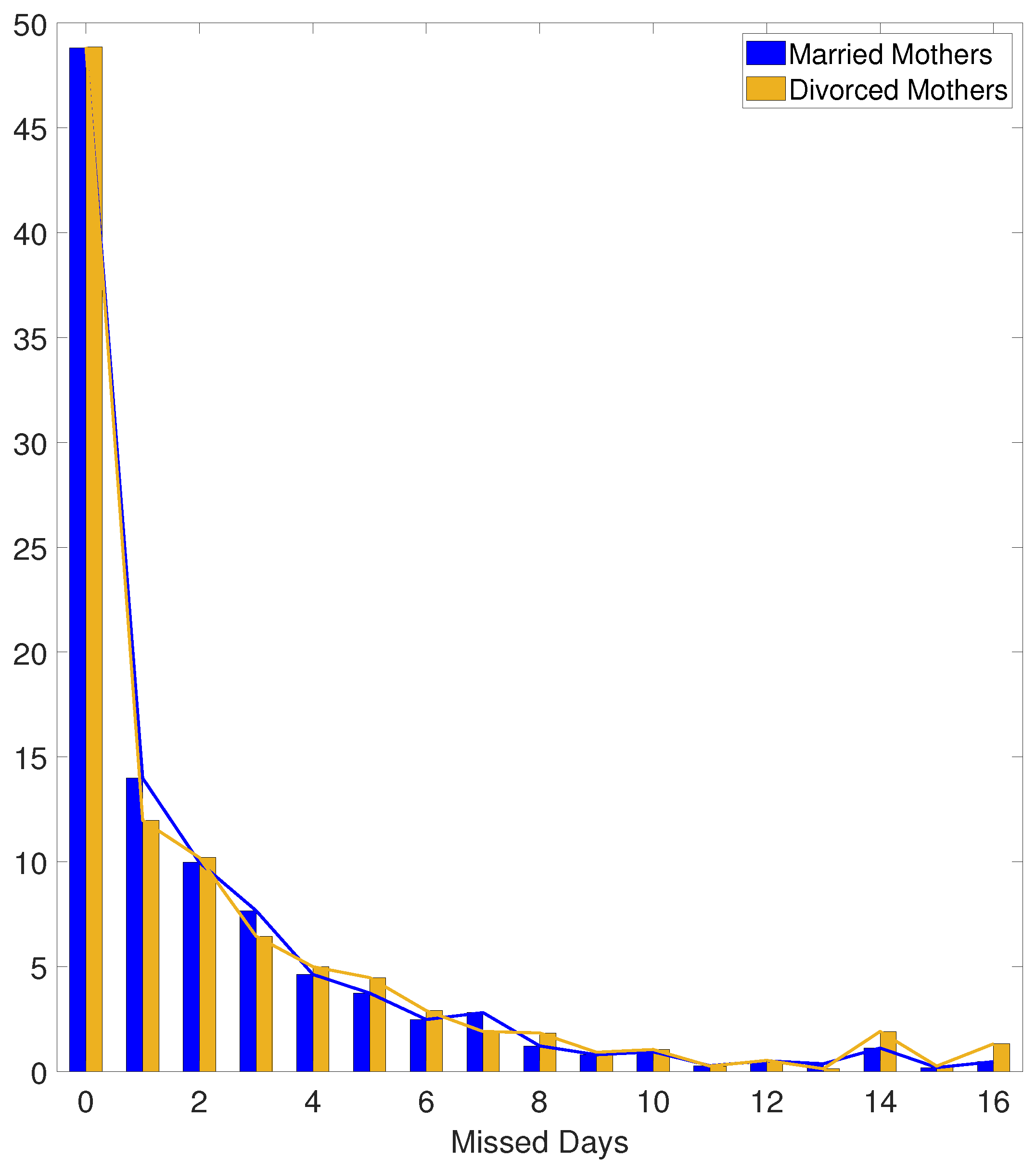
Figure 1 shows differences in the frequencies across married versus unmarried groups. The unmarried mothers group has a larger mean (2.211 versus 1.951) and dispersion (standard deviation of 3.480 versus 3.044). Overall, however, the distributions are very similar.

4.2. Results

The FMR model is estimated with two latent components in both the treated and untreated states, subject to inequality constraints. Separation of the components takes place based on the means and weights. The corresponding posterior distributions produce evidence of convergence. In the treated state, the component means are $1.361$ and $4.289$, with corresponding probabilities of $0.480$ and $0.520$. In the untreated state, the estimated component means are $1.940$ and $5.694$, and the associated probabilities are $0.464$ and $0.536$, respectively. Thus, whether married or unmarried, the substantially larger means for the second components suggest that those children missing more school are relatively less healthy than children in the first component. Further, the mixing probabilities suggest that the unhealthy components are slightly larger. The chains show good convergence, although the covariance parameters are slower to converge as expected. The Markov chains for them display relatively more persistent serial correlations.

Table 2. Posterior means and standard deviations of component parameters ${\mathit{\gamma }}_{12}$ (treated); ${\mathit{\gamma }}_{22}$ (untreated).

	Married Mothers		Unmarried Mothers
	Vector ${\mathit{\gamma }}_{\mathbf{12}}$		Vector  ${\mathit{\gamma }}_{\mathbf{22}}$
	Mean	Std. Dev.	Mean	Std. Dev.
CONST	$-0.797$	$0.295$	$-0.853$	$0.230$
chronic1	$0.791$	$0.286$	$0.822$	$0.216$
chronic2	$1.074$	$0.381$	$1.140$	$0.288$
chronic3	$1.465$	$0.523$	$1.209$	$0.333$
chronic4	$2.074$	$0.877$	$1.597$	$0.518$
chronic5	$1.633$	$0.885$	$2.990$	$1.692$
chronic6plus	$1.957$	$0.966$	$3.807$	$1.823$
PROB $j=2$	$0.480$	$0.041$	$0.464$	$0.034$

,

Table 3. Posterior means and standard deviations of parameters ${\mathit{\beta }}_{1j}$, ${\mathit{\beta }}_{2j}$, ${\delta }_{1j}$, ${\delta }_{2j}$, ${\sigma }_{1j}^2$, ${\sigma }_{2j}^2$ by state $\left(d=0,1\right)$ and components $\left(j=1,2\right)$.

	Married Mothers				Unmarried Mothers
	Component 1		Component 2		Component 1		Component 2
	Mean	Std. Dev.	Mean	Std. Dev.	Mean	Std. Dev.	Mean	Std. Dev.
CONST	$2.008$	$1.127$	$1.744$	$0.332$	$1.762$	$0.979$	$0.863$	$0.294$
famsize	$-0.402$	$0.166$	$-0.113$	$0.054$	$-0.696$	$0.195$	$-0.116$	$0.044$
agekid	$-1.874$	$0.693$	$-0.285$	$0.264$	$-0.413$	$0.573$	$0.144$	$0.173$
femalekid	$0.155$	$0.279$	$0.018$	$0.095$	$0.640$	$0.341$	$0.157$	$0.092$
bmikid	$-0.026$	$0.035$	$0.009$	$0.010$	$-0.067$	$0.039$	$0.008$	$0.008$
employedmom	$0.622$	$0.408$	$-0.140$	$0.110$	$-0.502$	$0.344$	$-0.341$	$0.100$
${\delta }_{tj}$ $(t=1,2)$	$-0.935$	$0.435$	$-0.288$	$0.156$	$-0.766$	$0.384$	$-0.343$	$0.113$
${\sigma }_{tj}^2$ $(t=1,2)$	$1.651$	$0.652$	$0.748$	$0.702$	$1.664$	$0.569$	$0.576$	$0.586$
$Eexp\left({\mu }_j^t\right)$	$1.361$	$0.613$	$4.289$	$1.156$	$1.940$	$0.556$	$5.694$	$1.028$

and

Table 4. Posterior means and standard deviations of the treatment equation parameter $\mathit{\alpha }$.

	Treatment Equation
	Parameter $\mathbf{\alpha }$
	Mean	Std. Dev.
famsize	$0.258$	$0.015$
agemom	$0.358$	$0.032$
bmimom	$-0.019$	$0.003$
blackmom	$-1.095$	$0.060$
hispmom	$-0.428$	$0.052$
vegoodmom	$-0.013$	$0.059$
goodmom	$-0.094$	$0.058$
fairmom	$-0.112$	$0.080$
poormom	$-0.410$	$0.158$
employedmom	$0.289$	$0.064$

present posterior means and standard deviations based on 50,000 replications with the burn-in phase of 1000 replications.

Table 2 reports estimates from Equation (3) which deal with component assignment. Parameters ${\mathit{\gamma }}_{12}$ and ${\mathit{\gamma }}_{22}$ increase the probabilities of the second components (higher mean). In addition to including self-perceived health variables vegoodkid, goodkid, fairkid, we include indicators chronic1, chronic2, chronic3, chronic4, chronic5 and chronic6plus for 1, 2, 3, 4, 5 and 6 or more chronic conditions (no chronic conditions is excluded). Not surprisingly, estimates suggest that a larger number chronic conditions is more likely to place an individual to the second component. By contrast, after controlling for chronic conditions, self-reported measures of child’s health exert minimal impact on component assignments.

Table 3 reports estimates from the outcome (missed days) equations. The variable famsize appears to exert a strong negative impact on missed days for all four treatment/component groups. No other variable has a strong impact in the healthy component in either treatment state, with the exception of agekid, which negatively affects missed days for married mothers. However, in the higher mean groups interpreted as relatively unhealthy, employedmom has a strong negative effect for unmarried mothers. Health status variables do not affect missed days in any of the groups. Midwest and northeast have positive impacts only for unmarried mothers in the unhealthy group.

Table 4 reports estimates from the treatment status Equation (2). The probability of being married is strongly and positively affected by family size, age of the mother, mother’s employment status and being from the south or midwest. Being black or Hispanic decreases the probability of being married. Poor health status and body mass index also negatively affect marital status.

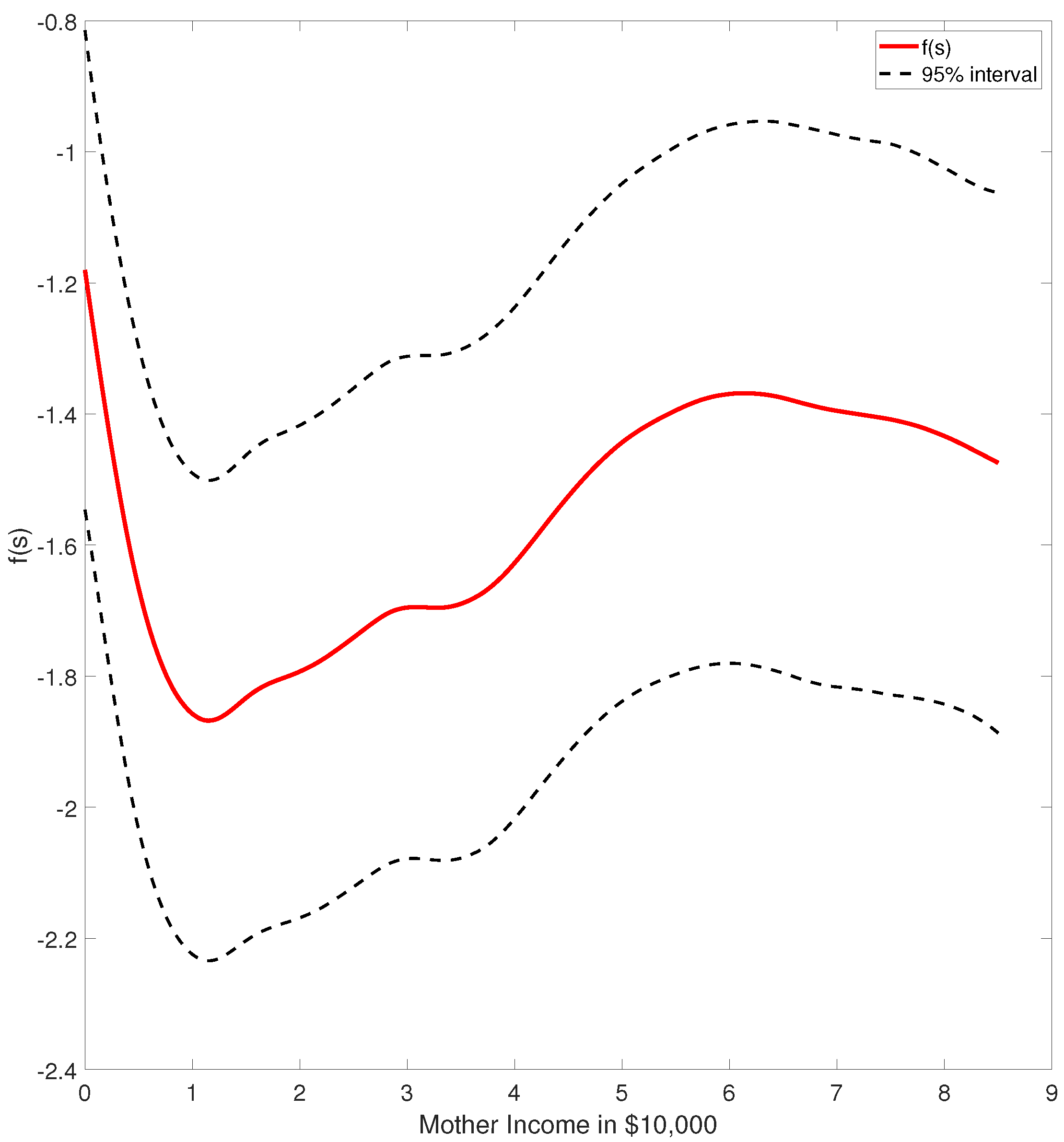
Figure 2 illustrates the estimated function $f\left(s_i\right)$ with the dashed lines giving the 95% posterior probability intervals. Its precisely estimated shape, coupled with its nonlinear form, help drive identification. The figure illustrates that incomemom has a long right tail with 95% of observations not exceeding the annual income of $85,000. Further, 5% of observations range between $85,000 and $260,000 and are very sparse, resulting in very imprecise nonparametric estimates. Therefore, we truncate incomemom at $85,000 and round it up to $200 which gives $k_{\nu }=329$ distinct values. The actual variable incomemom is defined as mother’s income divided by 10,000. The linear specification predicts that incomemom has a positive impact on the probability of treatment. However, the probability of treatment is maximized when income is zero based on the nonparametric model; it then monotonically decreases from 0 to $11,000 where it reaches the minimum. Following this, it increases until $30,000 and stays flat until $35,000 after which it increases at an even higher rate until $60,000 reaching a local maximum. It then decreases at a small rate.

Estimates of parameters, ${\delta }_{11}$, ${\delta }_{12}$, ${\delta }_{21}$ and ${\delta }_{22}$ (posterior means and standard deviations) are given in Table 3 as $-0.935$ $\left(0.435\right)$, $-0.288$ $\left(0.156\right)$, $-0.766$ $\left(0.384\right)$ and $-0.343$ $\left(0.113\right)$ respectively. Only ${\delta }_{11}$ and ${\delta }_{22}$ show more than two standard deviation separation from zero. Therefore, we test the joint hypothesis $H_0:{\delta }_{11}=0$, ${\delta }_{12}=0$, ${\delta }_{21}=0$, ${\delta }_{22}=0$. The Bayes factor is calculated as

$$B_0={\displaystyle \frac{\pi ({\delta }_{11}^{*},{\delta }_{12}^{*},{\delta }_{21}^{*},{\delta }_{22}^{*}|\mathbf{y})}{\pi ({\delta }_{11}^{*},{\delta }_{12}^{*},{\delta }_{21}^{*},{\delta }_{22}^{*})}},$$

(5)

a Savage–Dickey density ratio (Verdinelli & Wasserman, 1995). The ratio includes the posterior density $\pi ({\delta }_{11}^{*},{\delta }_{12}^{*},{\delta }_{21}^{*},{\delta }_{22}^{*}|\mathbf{y})$ and the prior density $\pi ({\delta }_{11}^{*},{\delta }_{12}^{*},{\delta }_{21}^{*},{\delta }_{22}^{*})$ evaluated at the point ${\delta }_{11}^{*}=0,$${\delta }_{12}^{*}=0,$${\delta }_{21}^{*}=0,$${\delta }_{22}^{*}=0$. We reject the null hypothesis.

4.3. Average Treatment Effects

Roy models, by construction, allow the conditional mean function of the outcome to vary by treatment status, which means that the treatment measure is not included as a typical right-hand side variable. Thus, treatment effects of interest must be calculated, post estimation, from converged parameter estimates. To that end, we calculate the average treatment effect (ATE) and the average treatment effect for the treated (ATET) of maternal marital status on missed school days. The link between the observed $Y_i$ and counterfactual outcomes is

$$Y_i=d_i\underset{j=1}{\sum ^2}{I}_{\left\{z_{ij}^1=1\right\}}{Y}_{ij}^1+(1-d_i)\underset{j=1}{\sum ^2}{I}_{\left\{z_{ij}^2=1\right\}}{Y}_{ij}^2.$$

The expected outcome gains are calculated for a randomly chosen child (ATE) and for a child who receives the treatment (ATET). If maternal marital status were randomly assigned, then ATE would equal ATET. But because marital status is not randomly assigned, the two are likely to differ, with the magnitude and direction of that difference informing upon endogeneity bias. For the computational details on how to calculate $E\left[Y^1-Y^2|\mathbf{X}\right]$ (ATE) and $E\left[Y^1-Y^2|\mathbf{X},\mathbf{W},d=1\right]$ (ATET), see Munkin (2022). Specifically, we calculate the treatment effects at the posterior means of the model parameters.

The estimated ATE is $-0.274$ $\left(0.049\right)$, suggesting that for a randomly chosen child, having a married mother decreases annual missed school days by about 13 percent relative to the sample mean of missed days ($2.059$). The estimated ATET is $0.291$ $\left(0.026\right)$, an increase of 14 percent of missed school days for those families who “select” a family structure with both parents. The interpretation is that, while marital status associates with fewer missed days for a random family, the unobserved factors that drive families into treatment also increase missed school days. This is evidence of adverse selection.

5. Conclusions

This paper analyzes factors affecting school absenteeism using the Finite Mixture Roy model developed by Munkin (2022). The observed patterns of missed school days are fitted with finite mixture distributions. The Roy structure controls heterogeneity due to the mother’s marital status. Unobserved heterogeneity due to healthy and unhealthy children in the sample is handled by finite mixtures. Our main finding is that, while marital status decreases absenteeism by about 13 percent for a randomly chosen family, this relationship flips the direction of the effect for those families which "select" to have both parents.

From a policy perspective, these findings should help lawmakers enact more appropriately targeted reforms. Education research has long identified “negative family processess” as significant in terms of correlating to school absenteeism (Marlow & Rehman, 2021). Thus, policymakers might find it tempting to reduce absenteeism by addressing family structure, perhaps by promoting marriage or offering partner support. However, the results of this paper cast doubt upon whether such reforms would help. In fact, the change in sign of the treatment effects suggests that certain family-friendly policies, while possibly worthwhile for other reasons, might actually make absenteeism worse.

Instead, policymakers should investigate what those unobserved factors might be and design reforms that target those. A meta analysis by Marlow and Rehman (2021) offers pointers to what some of those might be. Examples include shared genetics, family stress, and parenting practices. Such factors are nearly impossible to observe in household surveys, but the results of this paper suggest that policies aimed at addressing them could aid in reducing absenteeism.

The FMR model can prove taxing to implement, because, in most modeling situations, it requires user written code. Further, while MCMC algorithms allow researchers to sidestep tricky optimization issues common to frequentist approaches, Bayesian methods do require researchers to exercise care to ensure that the Markov chains “stablize” properly. Those concerns notwithstanding, the estimation approach holds promise in a variety of settings. For example, our future research concerns seek to apply the method to other count data outcomes, such as patents awarded to technology firms and defects spotted during manufacturing processes.

References

1. Balfanz, R., & Byrnes, V. (2012). Chronic absenteeism: Summarizing what we know from nationally available data (Vol. 1, pp. 1–46). Johns Hopkins University Center for Social Organization of Schools. [Google Scholar]
2. Basch, C. (2011). Healthier students are better learners: A missing link in school reforms to close the achievement gap. Journal of School Health, 81, 593–598. [Google Scholar] [CrossRef]
3. Bock, J. (2002). Evolutionary demography and intrahousehold time allocation: School attendance and child labor among the Okavango Delta peoples of Botswana. American Journal of Human Biology, 14, 206–221. [Google Scholar] [CrossRef]
4. Bowen, N., & Bowen, G. (1999). Effects of crime and violence in neighborhoods and schools on the school behavior and performance of adolescents. Journal of Adolescent Research, 14, 319–342. [Google Scholar] [CrossRef]
5. Cabus, S., & De Witte, K. (2015). Does unauthorized school absenteeism accelerate the dropout decision? Evidence from a Bayesian duration model. Applied Economics Letters, 22, 266–271. [Google Scholar] [CrossRef]
6. Celeux, G., Hurn, M., & Robert, C. P. (2000). Computational and inferential difficulties with mixture posterior distributions. Journal of the American Statistical Association, 95, 957–970. [Google Scholar] [CrossRef]
7. Celeux, G., Kamary, K., Malsiner-Walli, G., Marin, J.-M., & Robert, C. P. (2019). Computational solutions for Bayesian inference in mixture models. In S. Frühwirth-Schnatter, G. Celeux, & C. P. Robert (Eds.), Handbook of mixture analysis (pp. 73–96). CRC Press. Chapter 5. [Google Scholar]
8. Chib, S. (1995). Marginal likelihood from the Gibbs output. Journal of the American Statistical Association, 90, 1313–1321. [Google Scholar] [CrossRef]
9. Coelho, R., Fischer, S., McKnight, F., Matteson, S., & Schwarts, T. (2015). The effects of early chronic absenteeism on third-grade academic achievement measures. Workshop in Public Affairs. University of Wisconsin–Madison. [Google Scholar]
10. d’Haultfoeuille, X., & Maurel, A. (2013). Inference on an extended Roy model, with an application to schooling decisions in France. Journal of Econometrics, 174, 95–106. [Google Scholar] [CrossRef]
11. Durán-Narucki, V. (2008). School building condition, school attendance, and academic achievement in New York City public schools: A mediation model. Journal of Environmental Psychology, 28, 278–286. [Google Scholar] [CrossRef]
12. Epstein, J., & Sheldon, S. (2002). Present and accounted for: Improving student attendance through family and community involvement. The Journal of Educational Research, 95, 308–318. [Google Scholar] [CrossRef]
13. Frühwirth-Schnatter, S. (2001). Markov chain Monte Carlo estimation of classical and dynamic switching and mixture models. Journal of the American Statistical Association, 96, 194–209. [Google Scholar] [CrossRef]
14. Frühwirth-Schnatter, S. (2004). Estimating marginal likelihoods for mixture and Markov switching models using bridge sampling techniques. The Econometrics Journal, 7, 143–167. [Google Scholar] [CrossRef]
15. Gershenson, S., Jacknowitz, A., & Brannegan, A. (2017). Are student absences worth the worry in U.S. primary schools? Education Finance and Policy, 12, 137–165. [Google Scholar] [CrossRef]
16. Geweke, J. (2007). Interpretation and inference in mixture models: Simple MCMC works. Computational Statistics & Data Analysis, 51, 3529–3550. [Google Scholar] [CrossRef]
17. Geweke, J., & Keane, M. (2007). Smoothly mixing regressions. Journal of Econometrics, 138, 252–291. [Google Scholar] [CrossRef]
18. Ginsburg, A., Jordan, P., & Chang, H. (2014, August). Absences add up: How school attendance influences student success. Attendance Works. ERIC. [Google Scholar]
19. Goodman, J. (2014). Flaking out: Student absences and snow days as disruptions of instructional time (No. w20221). NBER Working Paper. National Bureau of Economic Research. [Google Scholar]
20. Gottfried, M. (2010). Evaluating the relationship between student attendance and achievement in urban elementary and middle schools: An instrumental variables approach. American Educational Research Journal, 47, 434–465. [Google Scholar] [CrossRef]
21. Gottfried, M. (2011). The detrimental effects of missing school: Evidence from urban siblings. American Journal of Education, 117, 147–182. [Google Scholar] [CrossRef]
22. Gottfried, M. (2014). Can neighbor attributes predict school absences? Urban Education, 49, 216–250. [Google Scholar] [CrossRef]
23. Gottfried, M., & Kirksey, J. (2017). When students miss school: The role of timing of absenteeism on students’ test performance. Educational Researcher, 46, 119–130. [Google Scholar] [CrossRef]
24. Holbert, T., Wu, L., & Stark, M. (2002). School attendance initiative: The first 3 years, 1998-2000/01. U.S. Department of Justice, National Institute of Law Enforcement and Criminal Justice. Available online: https://www.ojp.gov/ncjrs/virtual-library/abstracts/school-attendance-initiative-first-3-years-199899-200001 (accessed on 1 December 2025).
25. Jasra, A., Holmes, C. C., & Stephens, D. A. (2005). Markov chain Monte Carlo methods and the label switching problem in Bayesian mixture modeling. Statistical Science, 20, 50–67. [Google Scholar] [CrossRef]
26. Jordan, P., & Chang, H. (2015, September). Mapping the early attendance gap: Charting a course for student success. Attendance Works. Available online: https://www.attendanceworks.org/wp-content/uploads/2017/05/Mapping-the-Early-Attendance-Gap_Final-4.pdf (accessed on 1 December 2025).
27. Kearney, C. (2008). School absenteeism and school refusal behavior in youth: A contemporary review. Clinical Psychology Review, 28, 451–471. [Google Scholar] [CrossRef]
28. Keller, R. T. (1983). Predicting absenteeism from prior absenteeism, attitudinal factors, and nonattitudinal factors. Journal of Applied Psychology, 68, 536. [Google Scholar] [CrossRef]
29. Kline, B., & Tobias, J. L. (2008). The wages of BMI: Bayesian analysis of a skewed treatment-response model with nonparametric endogeneity. Journal of Applied Econometrics, 23, 767–793. [Google Scholar] [CrossRef]
30. Koop, G., & Poirier, D. J. (2004). Bayesian variants of some classical semiparametric regression techniques. Journal of Econometrics, 123, 259–282. [Google Scholar] [CrossRef]
31. Koop, G., & Tobias, J. L. (2006). Semiparametric Bayesian inference in smooth coefficient models. Journal of Econometrics, 134, 283–315. [Google Scholar] [CrossRef]
32. Malkus, N. (2024). Long COVID for public schools: Chronic absenteeism before and after the pandemic. American Enterprise Institute. [Google Scholar]
33. Marlow, S. A., & Rehman, N. (2021). The relationship between family processes and school absenteeism and dropout: A meta-analysis. The Educational and Developmental Psychologist, 38, 3–23. [Google Scholar] [CrossRef]
34. Munkin, M. K. (2022). Count Roy model with finite mixtures. Journal of Applied Econometrics, 37, 1160–1181. [Google Scholar] [CrossRef]
35. Roy, A. D. (1951). Some thoughts on the distribution of earnings. Oxford Economic Papers, 3, 135–146. [Google Scholar] [CrossRef]
36. Sandefur, G. D., McLanahan, S., & Wojtkiewicz, R. A. (1992). The effects of parental marital status during adolescence on high school graduation. Social Forces, 71, 103–121. [Google Scholar] [CrossRef]
37. Verdinelli, I., & Wasserman, L. (1995). Computing Bayes factors using a generalization of the Savage–Dickey density ratio. Journal of the American Statistical Association, 90, 614–618. [Google Scholar] [CrossRef]
38. Vos, S. D. (2001). Family structure and school attendance among children 13–16 in Argentina and Panama. Journal of Comparative Family Studies, 32, 99–115. [Google Scholar] [CrossRef]
Figure 1. Histograms of missed school days for married mothers versus divorced.
Econometrics 14 00013 g001
Figure 2. The effect of mother’s income on missed school days.
Econometrics 14 00013 g002