Quantitative Assessment and Driving Force Analysis of Mangrove Forest Changes in China from 1985 to 2018 by Integrating Optical and Radar Imagery


Abstract
1. Introduction
2. Materials and Methods
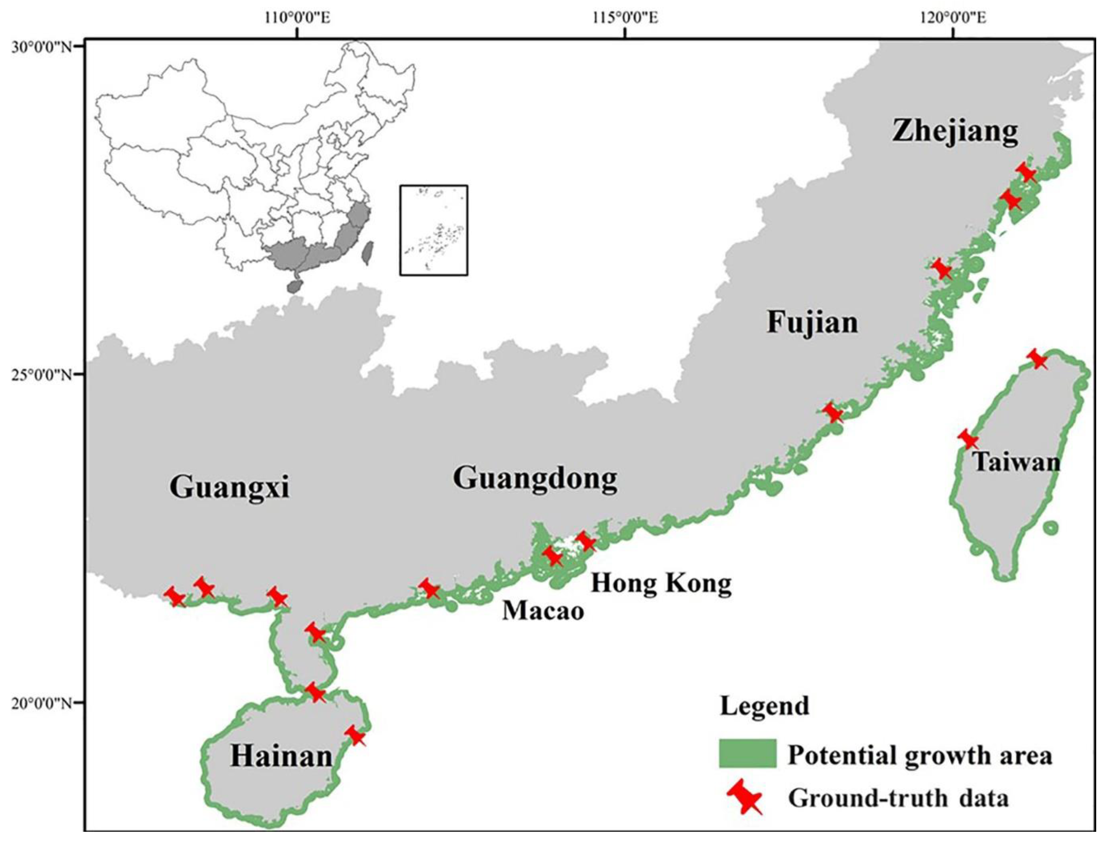
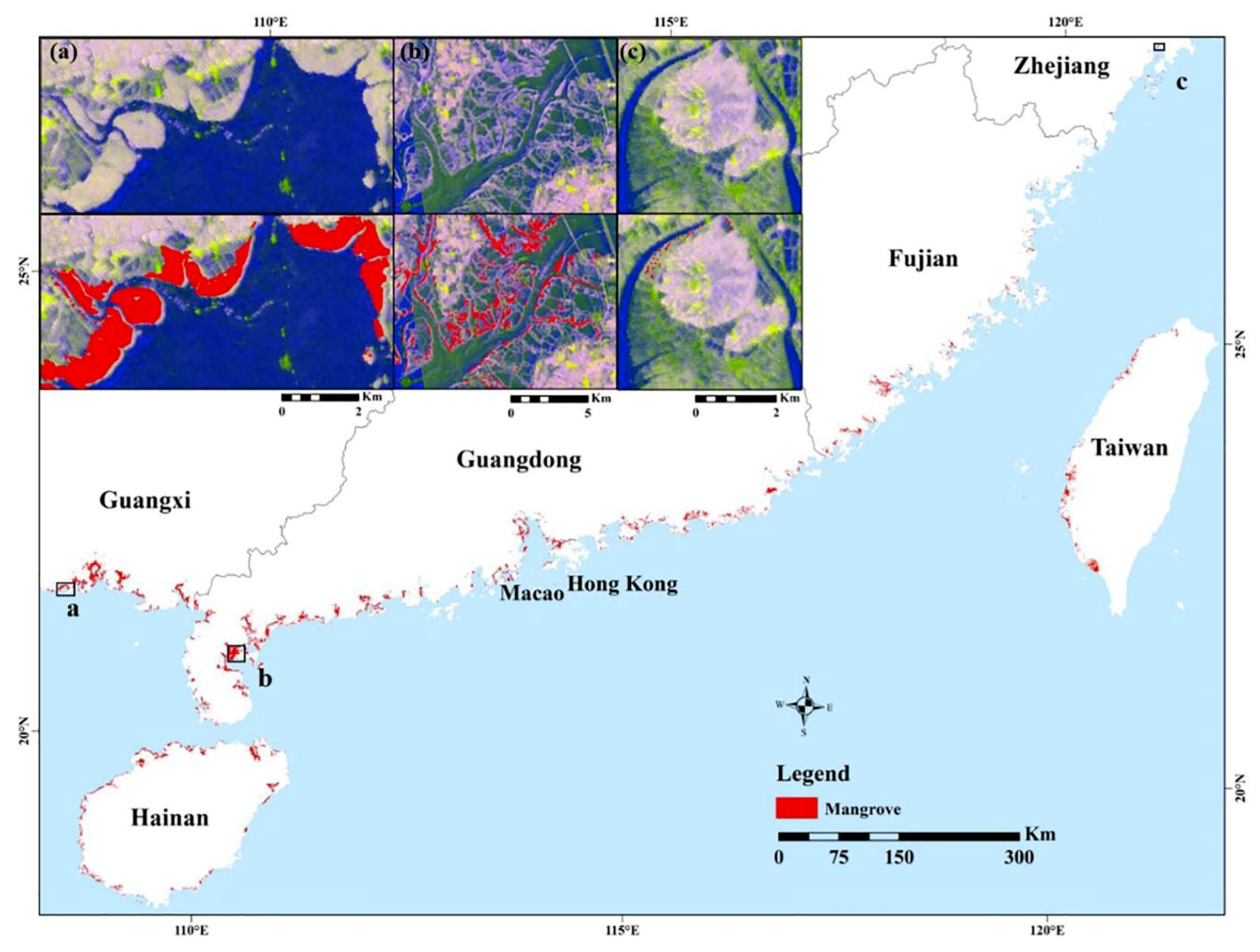
2.1. Study Area
2.2. Data
2.2.1. Synthetic Aperture Radar (SAR) Imagery
2.2.2. Landsat Imagery
2.2.3. Ground-Truth Data
2.2.4. Other Data
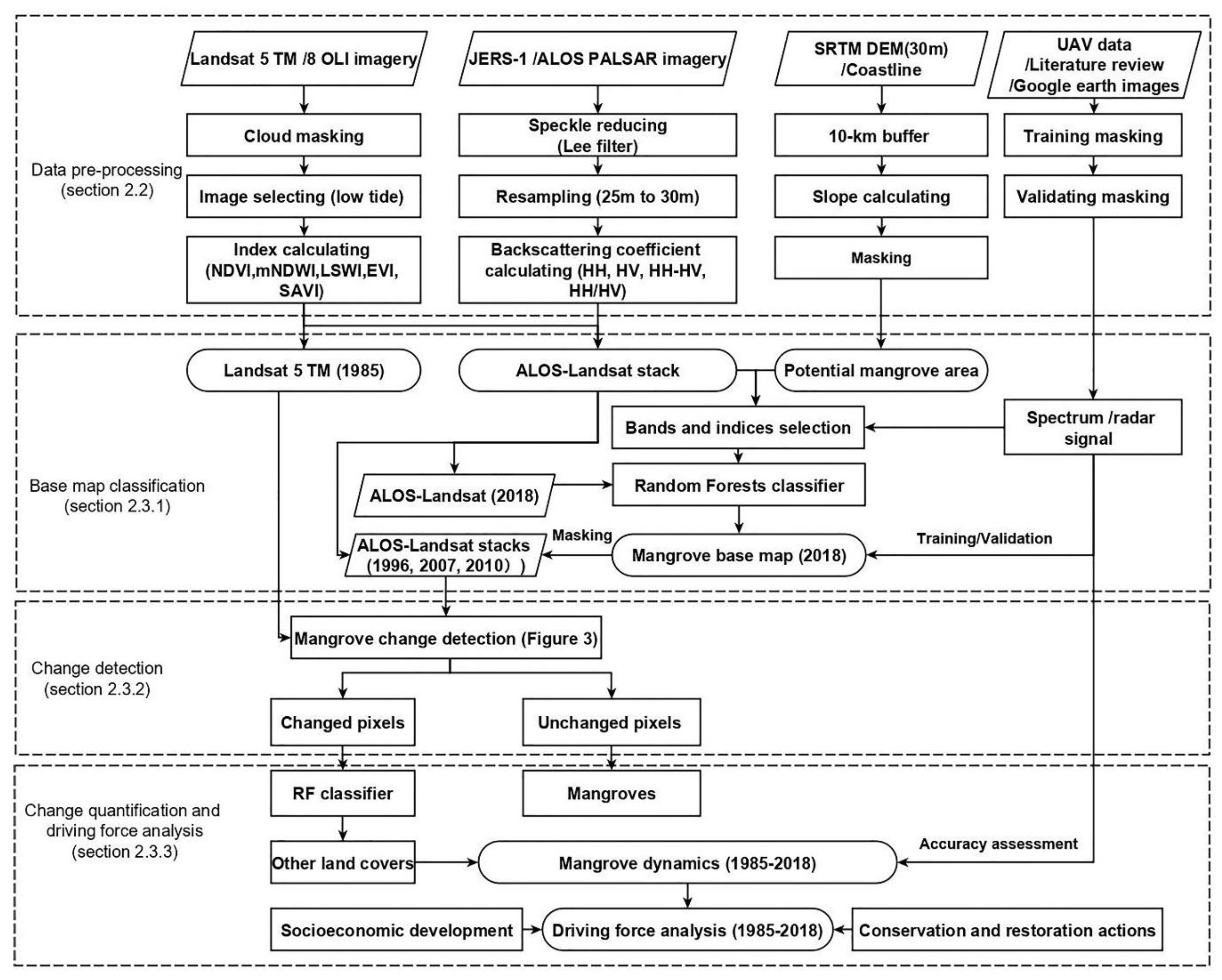
2.3. Methodology
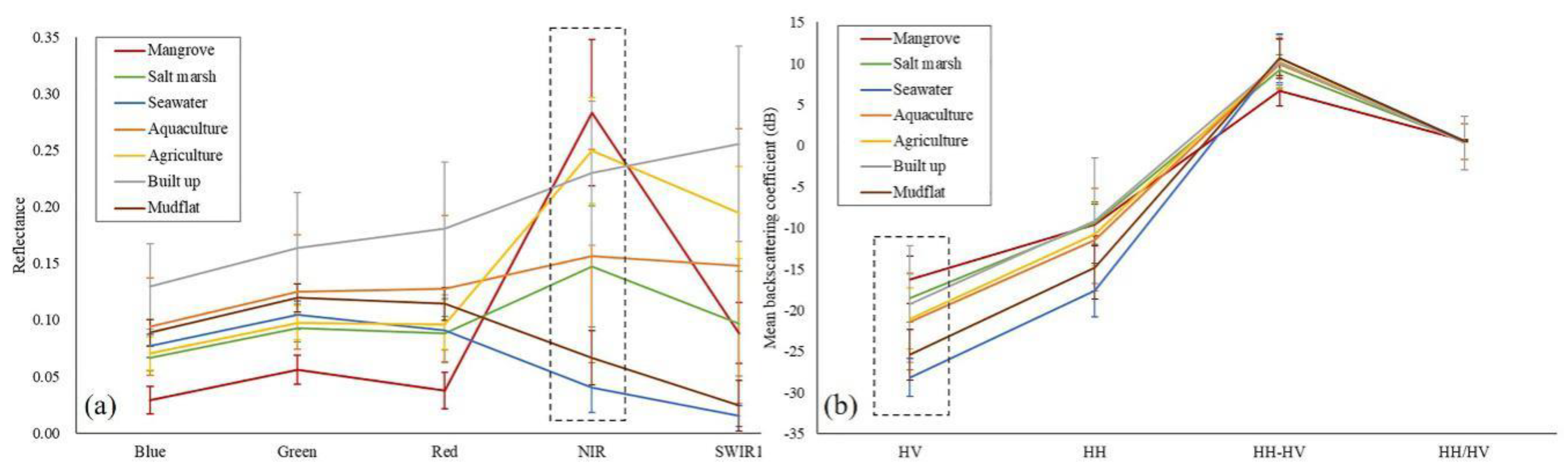
2.3.1. Mangrove Baseline Classification
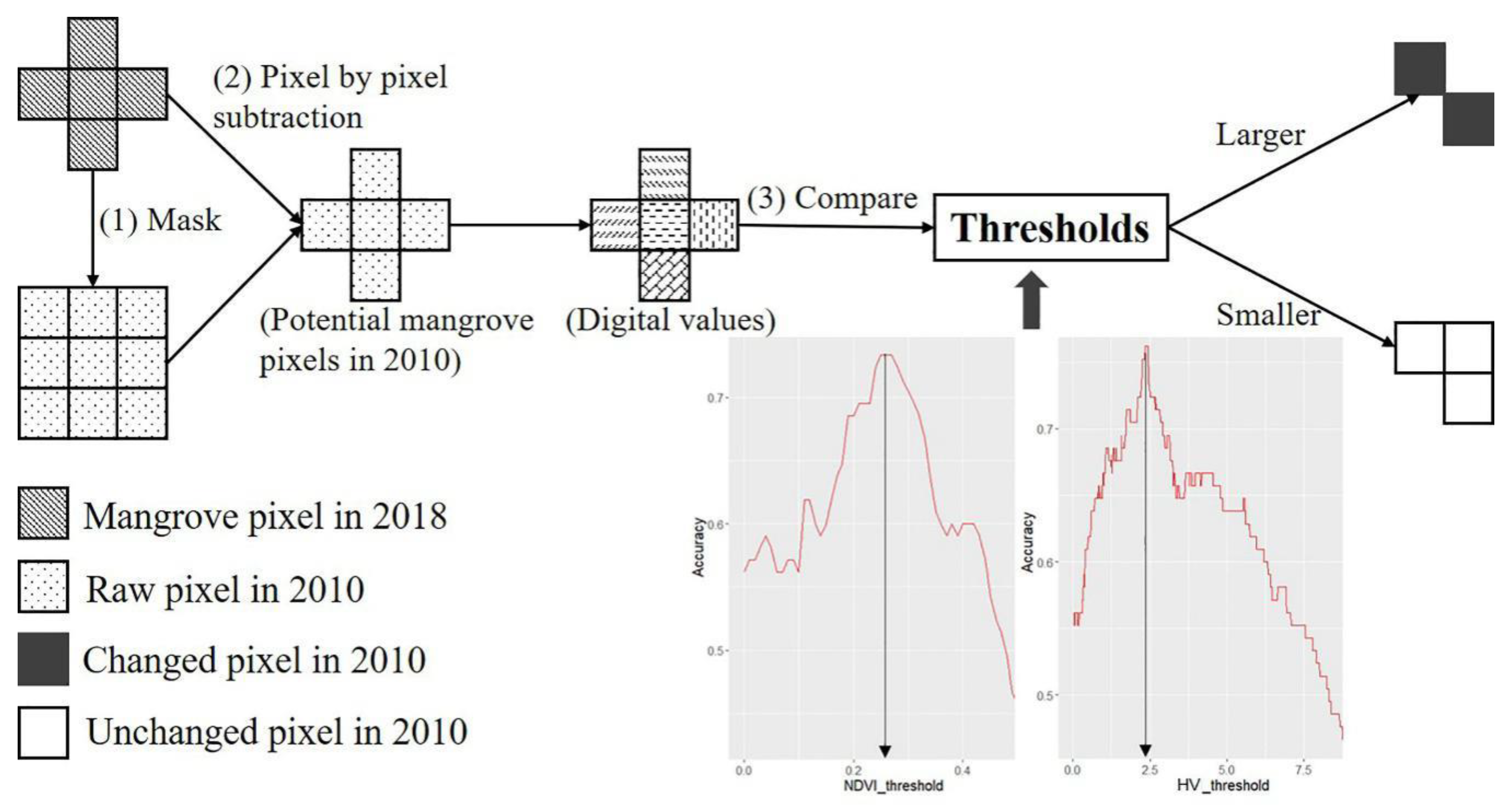
2.3.2. Mangrove Change Detection from 1985 to 2018
2.3.3. Quantitative Assessment of Mangrove Dynamics
3. Results
3.1. Mangrove Base Map
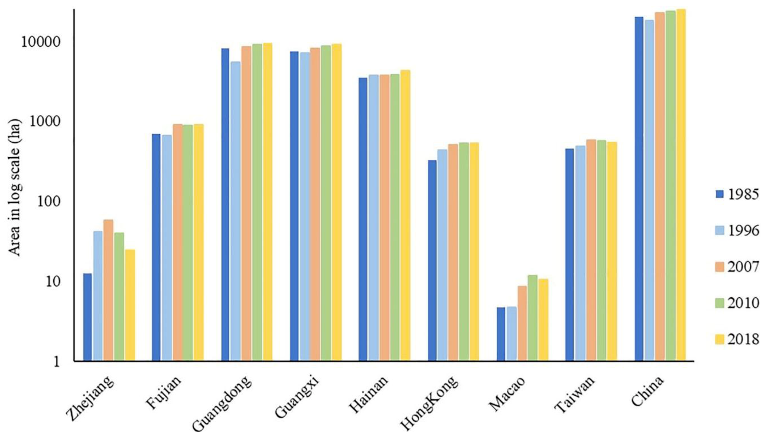
3.2. Mangrove Area Changes from 1985 to 2018
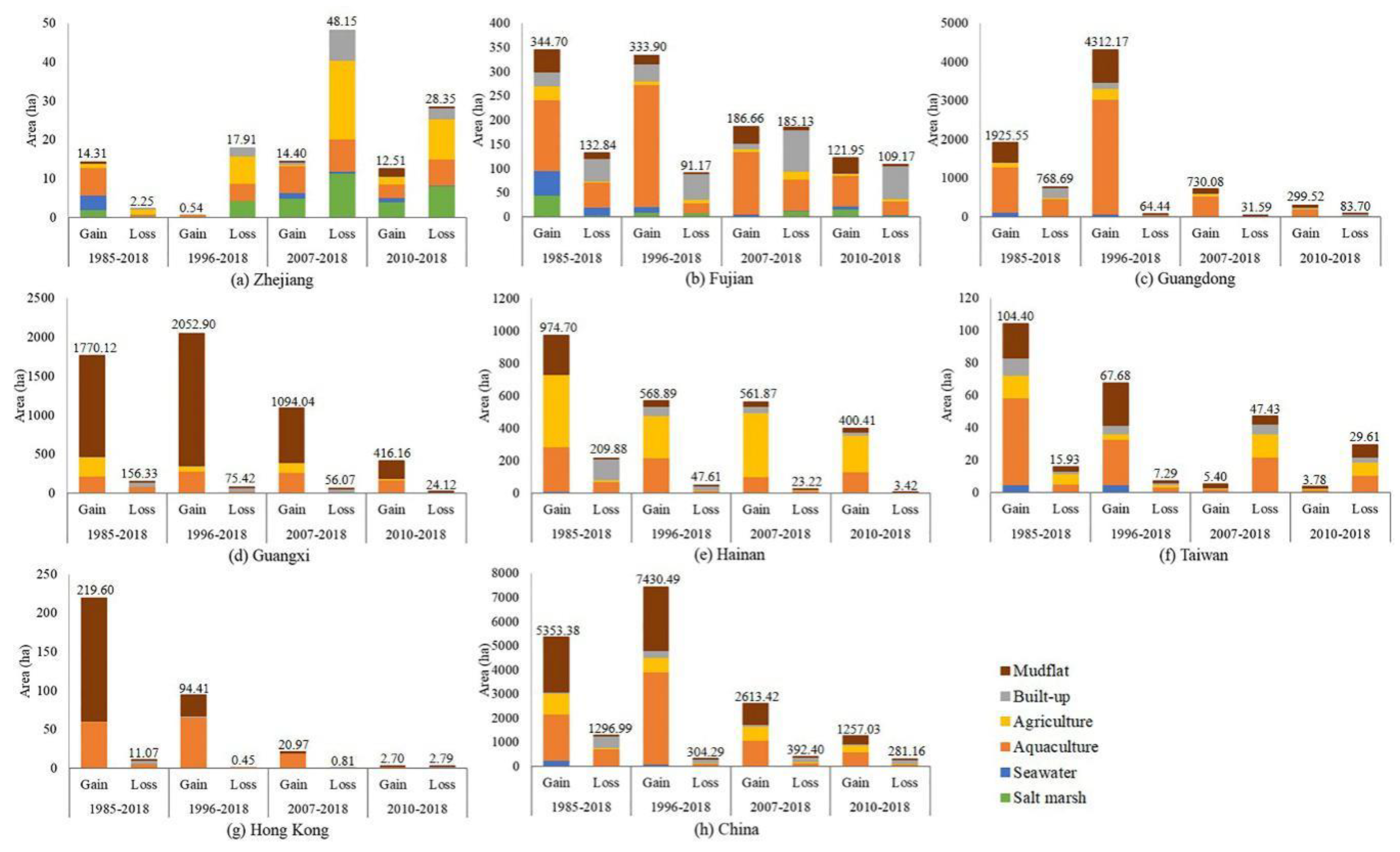
3.3. Quantitative Results of Mangrove Dynamics
4. Discussion
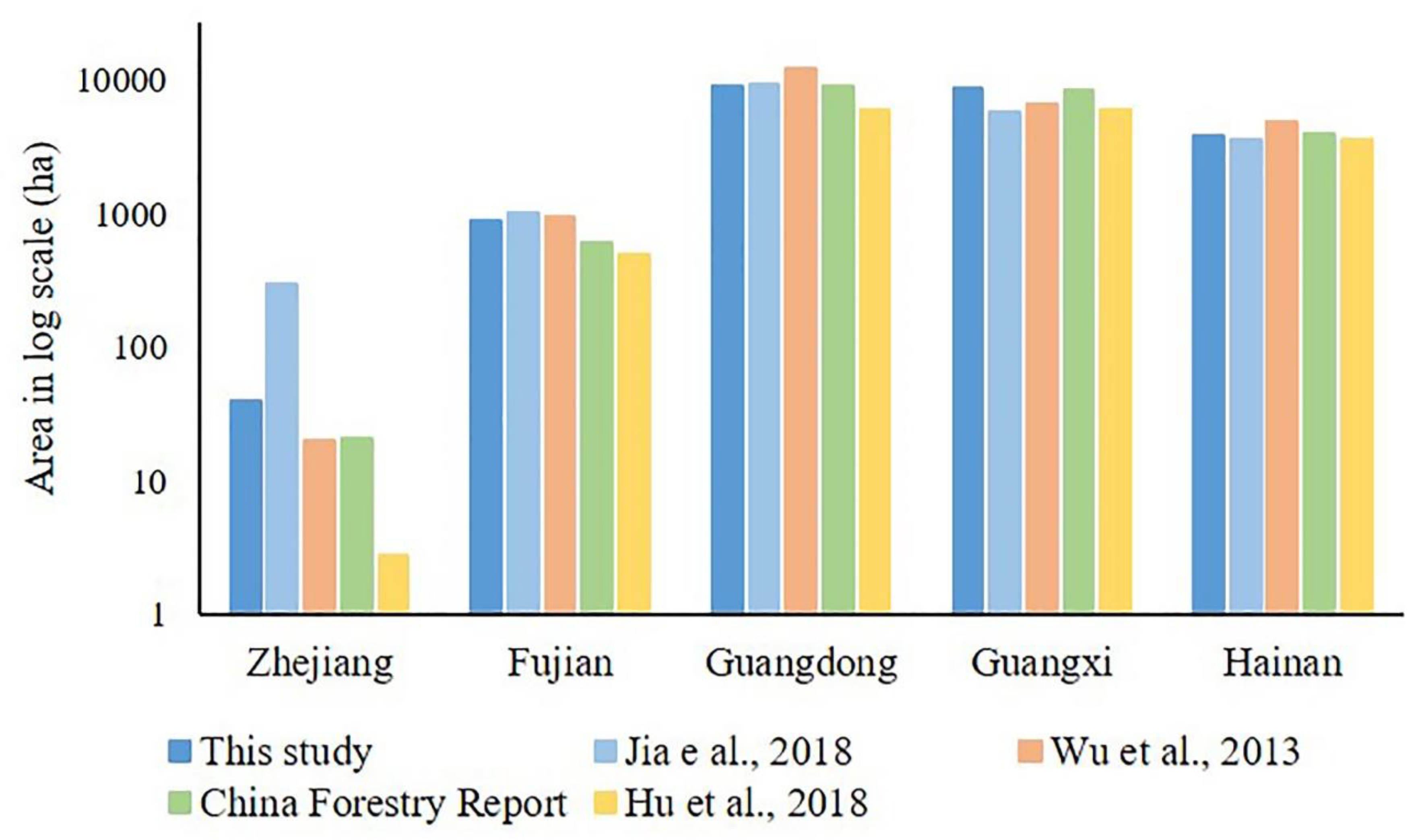
4.1. The Advantages in the Resultant Mangrove Dynamics
4.2. The Potential Sources of Uncertainties in the Resultant Mangrove Dynamics
4.3. The Possible Driving Forces of Mangrove Dynamics
5. Conclusions
Supplementary Materials
Author Contributions
Funding
Acknowledgments
Conflicts of Interest
Appendix A. Evaluation Accuracy after Classification

| MG | SW | AG | AQ | BU | MF | SM | ||
|---|---|---|---|---|---|---|---|---|
| MG | 44 | 14 | 0 | 2 | 0 | 0 | 4 | |
| SW | 6 | 56 | 0 | 0 | 0 | 0 | 0 | |
| AG | 0 | 4 | 36 | 0 | 0 | 0 | 4 | |
| Zhejiang | AQ | 6 | 2 | 0 | 34 | 0 | 0 | 0 |
| BU | 0 | 0 | 0 | 0 | 40 | 0 | 0 | |
| MF | 0 | 0 | 0 | 0 | 0 | 32 | 0 | |
| SM | 0 | 6 | 0 | 0 | 0 | 0 | 34 | |
| MG | 451 | 6 | 0 | 1 | 4 | 0 | 0 | |
| SW | 0 | 470 | 2 | 0 | 2 | 1 | 0 | |
| AG | 0 | 0 | 547 | 0 | 0 | 0 | 0 | |
| Fujian | AQ | 3 | 5 | 0 | 314 | 9 | 0 | 0 |
| BU | 5 | 8 | 0 | 1 | 343 | 2 | 0 | |
| MF | 1 | 0 | 0 | 0 | 4 | 586 | 0 | |
| SM | 0 | 8 | 5 | 0 | 0 | 0 | 274 | |
| MG | 1203 | 0 | 0 | 29 | 8 | 1 | 0 | |
| SW | 0 | 480 | 4 | 0 | 3 | 0 | 0 | |
| AG | 0 | 0 | 461 | 3 | 0 | 0 | 0 | |
| Guangdong | AQ | 22 | 0 | 3 | 719 | 5 | 29 | 2 |
| BU | 5 | 0 | 0 | 8 | 428 | 14 | 0 | |
| MF | 0 | 0 | 0 | 4 | 6 | 729 | 1 | |
| SM | 1 | 0 | 0 | 7 | 0 | 0 | 314 | |
| MG | 1666 | 0 | 2 | 1 | 1 | 0 | 0 | |
| SW | 0 | 376 | 3 | 4 | 0 | 0 | 0 | |
| AG | 1 | 0 | 616 | 3 | 0 | 0 | 0 | |
| Guangxi | AQ | 9 | 0 | 2 | 338 | 0 | 0 | 0 |
| BU | 1 | 0 | 0 | 0 | 231 | 0 | 0 | |
| MF | 0 | 0 | 0 | 0 | 0 | 379 | 0 | |
| SM | 0 | 0 | 0 | 0 | 0 | 0 | 0 | |
| MG | 1068 | 0 | 0 | 28 | 7 | 0 | 0 | |
| SW | 0 | 350 | 2 | 3 | 1 | 0 | 0 | |
| AG | 0 | 0 | 253 | 0 | 0 | 0 | 1 | |
| Hainan | AQ | 54 | 0 | 0 | 380 | 3 | 0 | 0 |
| BU | 8 | 0 | 0 | 19 | 203 | 1 | 0 | |
| MF | 1 | 0 | 0 | 0 | 0 | 120 | 0 | |
| SM | 0 | 0 | 1 | 2 | 0 | 0 | 80 |
| 1985 | 1996 | 2007 | 2010 | |||||
|---|---|---|---|---|---|---|---|---|
| Gain | Loss | Gain | Loss | Gain | Loss | Gain | Loss | |
| Zhejiang | 0.9590 | 0.9501 | 0.9481 | 0.9611 | 0.9628 | 0.9500 | 0.9595 | 0.9589 |
| Fujian | 0.9866 | 0.9632 | 0.9795 | 0.9005 | 0.9867 | 0.9553 | 0.9843 | 0.9712 |
| Guangdong | 0.9844 | 0.9487 | 0.9709 | 0.9445 | 0.9839 | 0.9546 | 0.9805 | 0.9581 |
| Guangxi | 1 | 0.9948 | 0.9993 | 0.9841 | 1 | 0.9888 | 0.9986 | 0.9809 |
| Hainan | 0.9581 | 0.9650 | 0.9480 | 0.9754 | 0.9862 | 0.9690 | 0.9794 | 0.9617 |
| Hong Kong | 0.9824 | 0.9605 | 0.9790 | 0.9472 | 0.9831 | 0.9552 | 0.9844 | 0.9605 |
| Taiwan | 0.9653 | 0.9676 | 0.9375 | 0.9690 | 0.9865 | 0.9565 | 0.9856 | 0.9725 |

References
- Nagelkerken, I.; van der Velde, G.; Gorissen, M.; Meijer, G.; Van’t Hof, T.; Den Hartog, C. Importance of mangroves, seagrass beds and the shallow coral reef as a nursery for important coral reef fishes, using a visual census technique. Estuar. Coast. Shelf Sci. 2000, 51, 31–44. [Google Scholar] [CrossRef]
- Arkema, K.K.; Guannel, G.; Verutes, G.; Wood, S.A.; Guerry, A.; Ruckelshaus, M.; Kareiva, P.; Lacayo, M.; Silver, J.M. Coastal habitats shield people and property from sea-level rise and storms. Nat. Clim. Chang. 2013, 3, 913–918. [Google Scholar] [CrossRef]
- Duarte, C.M.; Losada, I.J.; Hendriks, I.E.; Mazarrasa, I.; Marbà, N. The role of coastal plant communities for climate change mitigation and adaptation. Nat. Clim. Chang. 2013, 3, 961–968. [Google Scholar] [CrossRef]
- Murray, B.C.; Pendleton, L.; Jenkins, W.A.; Sifleet, S. Green Payments for Blue Carbon: Economic Incentives for Protecting Threatened Coastal Habitats. 2011. Available online: https://nicholasinstitute.duke.edu/environment/publications/naturalresources/blue-carbon-report (accessed on 6 July 2020).
- Hamilton, S.E.; Casey, D. Creation of a high spatio-temporal resolution global database of continuous mangrove forest cover for the 21st century (CGMFC-21). Glob. Ecol. Biogeogr. 2016, 25, 729–738. [Google Scholar] [CrossRef]
- Spalding, M.; Blasco, E.; Field, C. World Mangrove Alias; The International Society for Mangrove Ecosystems: Okinawa, Japan, 1997. [Google Scholar]
- Wu, J.; Zhang, H.; Pan, Y.; Krause-Jensen, D.; He, Z.; Fan, W.; Xiao, X.; Chung, I.; Marbà, N.; Serrano, O. Opportunities for blue carbon strategies in China. Ocean Coast. Manag. 2020, 194, 105241. [Google Scholar] [CrossRef]
- Li, X.; Yu, X.; Hou, X.; Liu, Y.; Li, H.; Zhou, Y.; Xia, S.; Liu, Y.; Duan, H.; Wang, Y. Valuation of Wetland Ecosystem Services in National Nature Reserves in China’s Coastal Zones. Sustainability 2020, 12, 3131. [Google Scholar] [CrossRef]
- He, Y.; Zhang, M. Study on wetland loss and its reasons in China. Chin. Geogr. Sci. 2001, 11, 241–245. [Google Scholar] [CrossRef]
- Spalding, M.; Kainuma, M.; Collins, L. World Atlas of Mangroves; Earthscan: London, UK, 2010. [Google Scholar]
- Giri, C.; Ochieng, E.; Tieszen, L.L.; Zhu, Z.; Singh, A.; Loveland, T.; Masek, J.; Duke, N. Status and distribution of mangrove forests of the world using earth observation satellite data. Glob. Ecol. Biogeogr. 2011, 20, 154–159. [Google Scholar] [CrossRef]
- Wu, P.; Zhang, J.; Ma, Y.; Li, X. Remote sensing monitoring and analysis of the changes of mangrove resource in China in the past 20 years. Adv. Mar. Sci. 2013, 31, 406–414, (In Chinese with English Abstract). [Google Scholar]
- Jia, M.; Wang, Z.; Li, L.; Song, K.; Ren, C.; Liu, B.; Mao, D. Mapping China’s mangroves based on an object-oriented classification of Landsat imagery. Wetlands 2014, 34, 277–283. [Google Scholar] [CrossRef]
- Chen, B.; Xiao, X.; Li, X.; Pan, L.; Doughty, R.; Ma, J.; Dong, J.; Qin, Y.; Zhao, B.; Wu, Z. A mangrove forest map of China in 2015: Analysis of time series Landsat 7/8 and Sentinel-1A imagery in Google Earth Engine cloud computing platform. ISPRS J. Photogramm. Remote Sens. 2017, 131. [Google Scholar] [CrossRef]
- Hu, L.; Li, W.; Xu, B. Monitoring mangrove forest change in China from 1990 to 2015 using Landsat-derived spectral-temporal variability metrics. Int. J. Appl. Earth Obs. Geoinf. 2018, 73, 88–98. [Google Scholar] [CrossRef]
- Jia, M.; Wang, Z.; Zhang, Y.; Mao, D.; Wang, C. Monitoring loss and recovery of mangrove forests during 42 years: The achievements of mangrove conservation in China. Int. J. Appl. Earth Obs. Geoinf. 2018, 73, 535–545. [Google Scholar] [CrossRef]
- Lee, J.-S. Digital image enhancement and noise filtering by use of local statistics. IEEE Trans. Pattern Anal. Mach. Intell. 1980, 165–168. [Google Scholar] [CrossRef]
- Tucker, C.J. Red and photographic infrared linear combinations for monitoring vegetation. Remote Sens. Environ. 1978, 8, 127–150. [Google Scholar] [CrossRef]
- Gao, B.-C. NDWI—A normalized difference water index for remote sensing of vegetation liquid water from space. Remote Sens. Environ. 1996, 58, 257–266. [Google Scholar] [CrossRef]
- Zhou, Y.; Xiao, X.; Qin, Y.; Dong, J.; Zhang, G.; Kou, W.; Jin, C.; Wang, J.; Li, X. Mapping paddy rice planting area in rice-wetland coexistent areas through analysis of Landsat 8 OLI and MODIS images. Int. J. Appl. Earth Obs. Geoinf. 2016, 46, 1–12. [Google Scholar] [CrossRef]
- Xu, H. Modification of normalised difference water index (NDWI) to enhance open water features in remotely sensed imagery. Int. J. Remote Sens. 2006, 27, 3025–3033. [Google Scholar] [CrossRef]
- Huete, A.R. A soil-adjusted vegetation index (SAVI). Remote Sensing of Environment. Remote Sens. Environ. 1988, 25, 295–309. [Google Scholar] [CrossRef]
- Bruzzone, L.; Prieto, D.F. Automatic analysis of the difference image for unsupervised change detection. IEEE Trans. Geosci. Remote Sens. 2000, 38, 1171–1182. [Google Scholar] [CrossRef]
- Dingle Robertson, L.; King, D.J. Comparison of pixel-and object-based classification in land cover change mapping. Int. J. Remote Sens. 2011, 32, 1505–1529. [Google Scholar] [CrossRef]
- Thomas, N.; Bunting, P.; Lucas, R.; Hardy, A.; Rosenqvist, A.; Fatoyinbo, T. Mapping mangrove extent and change: A globally applicable approach. Remote Sens. 2018, 10, 1466. [Google Scholar] [CrossRef]
- Macleod, R.D.; Congalton, R.G. A quantitative comparison of change-detection algorithms for monitoring eelgrass from remotely sensed data. Photogramm. Eng. Remote Sens. 1998, 64, 207–216. [Google Scholar]
- RStudio Team. RStudio: Integrated Development for R. RStudio; PBC: Boston, MA, USA, 2019. [Google Scholar]
- Chen, L.; Wang, W.; Zhang, Y.; Lin, G. Recent progresses in mangrove conservation, restoration and research in China. J. Plant Ecol. 2009, 2, 45–54. [Google Scholar] [CrossRef]
- Dong, J.; Xiao, X.; Menarguez, M.A.; Zhang, G.; Qin, Y.; Thau, D.; Biradar, C.; Moore III, B. Mapping paddy rice planting area in northeastern Asia with Landsat 8 images, phenology-based algorithm and Google Earth Engine. Remote Sens. Environ. 2016, 185, 142–154. [Google Scholar] [CrossRef]
- Held, A.; Ticehurst, C.; Lymburner, L.; Williams, N. High resolution mapping of tropical mangrove ecosystems using hyperspectral and radar remote sensing. Int. J. Remote Sens. 2003, 24, 2739–2759. [Google Scholar] [CrossRef]
- Ramsey, E.W.; Nelson, G.A.; Sapkota, S.K. Classifying coastal resources by integrating optical and radar imagery and color infrared photography. Mangroves Salt Marshes 1998, 2, 109–119. [Google Scholar] [CrossRef]
- Pham, T.D.; Yokoya, N.; Bui, D.T.; Yoshino, K.; Friess, D.A. Remote sensing approaches for monitoring mangrove species, structure, and biomass: Opportunities and challenges. Remote Sens. 2019, 11, 230. [Google Scholar] [CrossRef]
- Huang, X.; Peng, X.; Qiu, J.; Chen, S. Mangrove status and development prospects in southern Zhejiang Province. J. Zhejiang For. Coll. 2009, 26, 427–433, (In Chinese with English Abstract). [Google Scholar]
- Wang, A.; Chen, J.; Jing, C.; Ye, G.; Wu, J.; Huang, Z.; Zhou, C. Monitoring the invasion of Spartina alterniflora from 1993 to 2014 with Landsat TM and SPOT 6 satellite data in Yueqing Bay, China. PLoS ONE 2015, 10, e0135538. [Google Scholar] [CrossRef]
- Wang, L.; Jia, M.; Yin, D.; Tian, J. A review of remote sensing for mangrove forests: 1956–2018. Remote Sens. Environ. 2019, 231, 111223. [Google Scholar] [CrossRef]
- Jia, M.; Liu, M.; Wang, Z.; Mao, D.; Ren, C.; Cui, H. Evaluating the effectiveness of conservation on mangroves: A remote sensing-based comparison for two adjacent protected areas in Shenzhen and Hong Kong, China. Remote Sens. 2016, 8, 627. [Google Scholar] [CrossRef]
- Songsom, V.; Koedsin, W.; Ritchie, R.J.; Huete, A. Mangrove phenology and environmental drivers derived from remote sensing in southern Thailand. Remote Sens. 2019, 11, 955. [Google Scholar] [CrossRef]
- Liu, M.; Zhang, H.; Lin, G.; Lin, H.; Tang, D. Zonation and directional dynamics of mangrove forests derived from time-series satellite imagery in Mai Po, Hong Kong. Sustainability 2018, 10, 1913. [Google Scholar] [CrossRef]


| Dataset | Period | Resolution | Band | Source |
|---|---|---|---|---|
| Phased Array type L-band Synthetic Aperture Radar (PALSAR/PALSAR-2) | 2007, 2010, 2018 | 25 m | Horizontal transmit and Vertical receive (HV) | Japan Aerospace Exploration Agency (JAXA) |
| Japanese Earth Resources Satellite 1 (JERS-1) | 1996 | 25 m | Horizontal transmit and Horizontal receive (HH) | JAXA |
| Landsat 5 Thematic Mapper | 1985, 1996, 2007, 2010 | 30 m | B3, B4, B5 | United States Geological Survey (USGS) |
| Landsat 8 Operational Land Imager | 2018 | 30 m | B3, B4, B5, B6 | USGS |
| Shuttle Radar Topography Mission (v3) | 2000 | 30 m | - | National Aeronautics and Space Administration |
| OpenStreetMap | 2018 | - | - | OpenStreetMap Foundation |
| Area (ha) | Producer Accuracy (%) | User Accuracy (%) | Overall Accuracy (%) | Kappa Coefficient | |
|---|---|---|---|---|---|
| Zhejiang | 24.48 | 88.89 ± 11.11 | 86.69 ± 13.31 | 85.19 ± 12.21 | 0.8251 |
| Fujian | 908.55 | 97.85 ± 3.28 | 97.37 ± 2.63 | 97.80 ± 2.96 | 0.9741 |
| Guangdong | 9217.63 | 96.87 ± 3.49 | 96.73 ± 4.55 | 96.55 ± 4.02 | 0.9583 |
| Guangxi | 9095.71 | 99.25 ± 1.56 | 98.95 ± 2.10 | 99.26 ± 1.83 | 0.9897 |
| Hainan | 4269.78 | 96.29 ± 8.32 | 95.02 ± 8.06 | 94.93 ± 8.19 | 0.9321 |
| Hong Kong | 533.34 | 98.89 ± 2.52 | 99.06 ± 1.76 | 99.02 ± 2.14 | 0.9794 |
| Macao | 10.62 | - | - | - | - |
| Taiwan | 542.34 | 87.72 ± 12.01 | 94.52 ± 9.52 | 93.83 ± 10.77 | 0.8115 |
| Total | 24,602.45 | - | - | 95.23 ± 6.02 | 0.9243 |
| SW (ha) | AG (ha) | AQ (ha) | BU (ha) | MF (ha) | SM (ha) | Total (ha) | Net (ha) | |||
|---|---|---|---|---|---|---|---|---|---|---|
| 1985 | Loss | MG | −30 | −46 | −692 | −493 | −31 | −4 | −1297 | 4057 |
| Gain | 195 | 853 | 1934 | 61 | 2263 | 47 | 5353 | |||
| 1996 | Loss | MG | −7 | −27 | −107 | −141 | −7 | −14 | −303 | 7128 |
| Gain | 101 | 608 | 3807 | 278 | 2626 | 11 | 7431 | |||
| 2007 | Loss | MG | −6 | −55 | −120 | −174 | −12 | −25 | −392 | 2222 |
| Gain | 24 | 589 | 1048 | 73 | 874 | 6 | 2614 | |||
| 2010 | Loss | MG | −3 | −35 | −82 | −134 | −15 | −12 | −281 | 976 |
| Gain | 25 | 278 | 562 | 42 | 330 | 20 | 1257 |
© 2020 by the authors. Licensee MDPI, Basel, Switzerland. This article is an open access article distributed under the terms and conditions of the Creative Commons Attribution (CC BY) license (http://creativecommons.org/licenses/by/4.0/).
Share and Cite
Zheng, Y.; Takeuchi, W. Quantitative Assessment and Driving Force Analysis of Mangrove Forest Changes in China from 1985 to 2018 by Integrating Optical and Radar Imagery. ISPRS Int. J. Geo-Inf. 2020, 9, 513. https://doi.org/10.3390/ijgi9090513
Zheng Y, Takeuchi W. Quantitative Assessment and Driving Force Analysis of Mangrove Forest Changes in China from 1985 to 2018 by Integrating Optical and Radar Imagery. ISPRS International Journal of Geo-Information. 2020; 9(9):513. https://doi.org/10.3390/ijgi9090513
Chicago/Turabian StyleZheng, Yuhan, and Wataru Takeuchi. 2020. "Quantitative Assessment and Driving Force Analysis of Mangrove Forest Changes in China from 1985 to 2018 by Integrating Optical and Radar Imagery" ISPRS International Journal of Geo-Information 9, no. 9: 513. https://doi.org/10.3390/ijgi9090513
APA StyleZheng, Y., & Takeuchi, W. (2020). Quantitative Assessment and Driving Force Analysis of Mangrove Forest Changes in China from 1985 to 2018 by Integrating Optical and Radar Imagery. ISPRS International Journal of Geo-Information, 9(9), 513. https://doi.org/10.3390/ijgi9090513