Abstract
Seagrass provides a wide range of essential ecosystem services, supports climate change mitigation, and contributes to blue carbon sequestration. This resource, however, is undergoing significant declines across the globe, and there is an urgent need to develop change detection techniques appropriate to the scale of loss and applicable to the complex coastal marine environment. Our work aimed to develop remote-sensing-based techniques for detection of changes between 1990 and 2019 in the area of seagrass meadows in Tauranga Harbour, New Zealand. Four state-of-the-art machine-learning models, Random Forest (RF), Support Vector Machine (SVM), Extreme Gradient Boost (XGB), and CatBoost (CB), were evaluated for classification of seagrass cover (presence/absence) in a Landsat 8 image from 2019, using near-concurrent Ground-Truth Points (GTPs). We then used the most accurate one of these models, CB, with historic Landsat imagery supported by classified aerial photographs for an estimation of change in cover over time. The CB model produced the highest accuracies (precision, recall, F1 scores of 0.94, 0.96, and 0.95 respectively). We were able to use Landsat imagery to document the trajectory and spatial distribution of an approximately 50% reduction in seagrass area from 2237 ha to 1184 ha between the years 1990–2019. Our illustration of change detection of seagrass in Tauranga Harbour suggests that machine-learning techniques, coupled with historic satellite imagery, offers potential for evaluation of historic as well as ongoing seagrass dynamics.
1. Introduction
Seagrass provides a number of valuable ecosystem services in coastal areas, including primary production, biogenic habitat production, water filtering, wave energy attenuation, and sediment trapping [1,2]. In recent years, blue carbon, including seagrass meadows, has been acknowledged as an important service for climate change mitigation because of its value in the sequestration of carbon [3,4]. Seagrass meadows, however, have declined and degraded across most regions in the world, a change largely attributed to anthropogenic effects [5,6,7].
The destruction of seagrass leads to the loss of various ecosystem services [7,8] and threatens the stability [6] and long-term livelihood of the fisherman in coastal areas [9,10]. Therefore, an accurate and rapid technique to inventory this resource is in high demand [5,11,12], to contribute baseline data for the evaluation of coastal ecosystem dynamics, establishment of marine protected areas, and functional zoning fitting to the local conditions. Where this can include a historic perspective, it can provide a comprehensive understanding of system change.
Several attempts at mapping and monitoring seagrass meadows using different satellite sensors and approaches have been reported [12]. Change of seagrass cover has been assessed using RapidEye [13], Indian satellite image (IRS LISS IV) [14], WorldView-2, IKONOS, Quickbird-2 [15], and Landsat [16,17,18,19] in various parts of the globe including the Mediterranean, the USA, Australia, and Malaysia. The temporal range of these attempts is constrained by the various platform launch dates, and typically range from 5 to around 25 years. Few efforts have attempted a longer-term change detection (30–40 years) of seagrass, and accuracy assessment has not frequently been reported for such long-term change detection. The reasons for this may relate to a deficiency of ground-truth data against which to evaluate older satellite scenes, and a need for imagery for the development of robust models for the classification of seagrass meadows in variably submerged conditions to be captured at optimal times to allow traditional classification procedures to be applied.
In recent years, machine learning (ML) has been emerging as an effective approach in various classification tasks, including for seagrass mapping [12,20]. ML provides improvements over the traditional Earth observation (EO) data classification approaches, to deal better with the challenges of mixed habitat, coarse spatial resolution of satellite imagery, and water column and atmospheric interference in coastal habitats [20,21,22]. Advantages of ML models are their use of non-parametric approaches, requiring no assumptions of normal distribution of input data, effective use of noisy data, and capability for multiple feature extraction [23,24,25,26]. The application of ML techniques to multitemporal satellite data, gathered from different satellite platforms, may therefore improve the overall accuracy of the classification result and enhance the reliability of seagrass change assessment. A range of different ensemble-based supervised classification techniques, such as boosting and bagging approaches [21,22,23,24], have been considered and tested in the literature for this type of task [27,28]. The most important differences between the bagging and boosting methods come from the approaches to the creation of training and testing datasets, and how the bagging and boosting methods deal with weak learners during the learning process [29,30]. Despite the potential for improved classification accuracy in suboptimal datasets, these approaches have not yet been fully implemented for seagrass change detection [12]. We are aware of only a single study, using Random Forest (RF) classification, for mapping the change of seagrass cover [13]. In the case study reported by these authors, the performance of the model was unstable and the accuracy varied among acquired scenes. Here we test the performance of a range of ML models, both boosting and bagging methods, with a time-series of satellite images, to compare their performances for assessment of seagrass cover and long-term change in Tauranga Harbour. Our goal is to improve the accuracy of tools for seagrass mapping and change detection.
Landsat time-series data were selected for the current study as the longest available time series and as freely available satellite remotely sensed resources. Landsat has operated since 1972 and provides continuous, homogeneous input data up to the most current Landsat 8 operational land imager (OLI) in orbit [31]. The Landsat multitemporal data has been used previously for several long-term change detection tasks [12,32] with the combination of long-term acquisition, medium spatial resolution, and the high quality of atmosphere-corrected products cited as important attributes. The spatial resolution has been retained as 30 m through eight generations (Landsat 1–Landsat 8); however, the radiometric resolution has been improved from 8 bit to 12 bit, leading to a better recognition of surface objects [33]. In addition, Landsat imagery includes blue, green, and red wavebands, which are the most appropriate for underwater resource mapping [34,35,36], but have not yet been evaluated for long-term seagrass change detection [12]. Thus, our work attempts to fill a gap in the current literature by assessing the performance of historic Landsat imagery, coupled with various machine-learning boosting and bagging models implemented in an open-source environment, in mapping changes in seagrass extent in a tidally inundated environment.
We employed two well-known models, i.e., Support Vector Machine (SVM), Random Forests (RF); and two novel techniques, Extreme Gradient Boosting (XGB), and CatBoost (CB) for the classification of seagrass meadows in Tauranga Harbour from Landsat imagery, and for detecting change across 29 years. The results demonstrated that the novel classification method CB was successful in describing the dynamics of change in seagrass in the study site as well as contributing baseline data for further assessment of change.
2. Materials and Methods
2.1. Study Site
We selected Tauranga Harbour (North Island, New Zealand) as the study site (Figure 1), due to its large size (201 km2 in surface area [37]), variation in water depth (from 0 m when exposed to 20 m in deep channels [38]), widely distributed but patchy seagrass cover and the availability of historic ground-truth information. The tidal regime is semidiurnal, with a range of 0.2–2.1 m, and the estuary has an average water residence time of 3–8 days [39]. Zostera muelleri is the only species of seagrass, occurring primarily in the intertidal parts of the harbor [20,37]. The growth rate of Z. muelleri is optimal at 12 practical salinity units (psu) [40] and 27–33 °C [41,42]. It attains its highest biomass in the austral summer and declines gradually over the winter, reaching a minimum cover in early spring [43]. Flowering and seed production of Z. muelleri is rare in New Zealand, reproduction is primarily vegetative and patch dynamics are correspondingly slow [44,45]. Seagrass is primarily intertidal in the estuary and, based on bathymetry and tidal predictions [38] at the time of the Landsat image acquisition, water depths ranged between 0.0–1.5 m in the locations where seagrass was present.
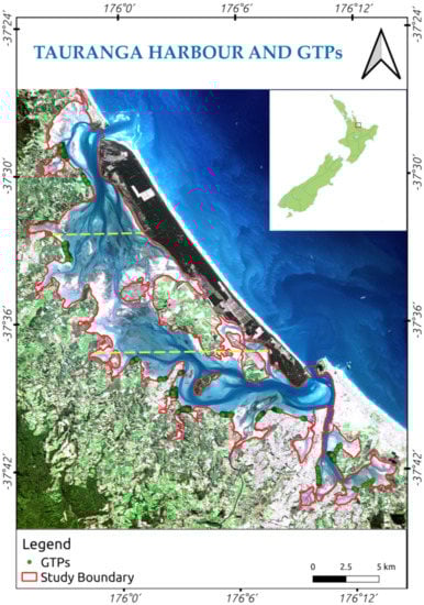
Figure 1.
Tauranga Harbour—our study site (ρRed—ρGeen—ρBlue composited Landsat image, date on 23 May 2019). Ground-Truth Points, collected on 1–7 April 2019, are indicated by green circles (yellow lines indicate the boundaries of the northern, central, and southern harbor).
In recent decades, Tauranga Harbour has been increasingly influenced by agricultural activities in the northern part (between 37.44° S and 37.54° S) and urban development in the southern part (between 37.62° S and 37.72° S). Episodic high loadings of sediment have been recorded and have resulted in the accumulation of sediment and high turbidity over the autumn and winter seasons [46,47]. Changes in the sedimentary environment have been implicated in negative impacts on the growth of seagrass [48,49], though other factors may also be involved. Available maps of seagrass in 1959, 1996, and 2011 derived from manual classification of aerial photography provided a resource for model validation [37].
2.2. Satellite Image Acquisition
Landsat images were downloaded from the GLOVIS website [50] for the years 1990, 2001, 2011, 2014, and 2019 (Table 1) at process level 1 (pixel value in digital number), and in the projection of WGS-84 UTM 60S. Landsat images were selected based on: (1) the acquired time of the Landsat image that coincided as closely as possible to low tide at the study site; (2) the image that had the lowest coverage of cloud; (3) whether there existed a similar acquisition month among the scenes. In practice, we selected scenes that ranged 1–2 months around March (Table 2).

Table 1.
Landsat data acquisitions used for seagrass mapping and change detection.
Table 2.
Available aerial, Google Earth images corresponding to historic Landsat images acquisition.
2.3. Field Survey Data
A field survey was undertaken from 1–7 April 2019 (Figure 1) in the intertidal areas of the harbor. At low tide, the boundary of seagrass meadows was delimited using a Global Positioning System (GPS) Garmin Etrex 30 with an accuracy of ±2 m. Other substrata recorded during the field survey were bare sand and muddy sand. Macroalgae were neither detected from our field survey nor mentioned in previous mapping reports [37,51].
Ground-Truth Points (GTPs), which were the base points to make the regions of interest (ROIs) for given classes, were recorded by following the boundary between seagrass meadows and non-vegetated areas. A total of 4315 GTPs were recorded for seagrass distribution, and 237 GTPs for other substrata in the harbor.
2.4. Ground-Truth Historical Scenes
Before 2019, no GTPs from field surveying were available, therefore we used aerial and Google Earth images (Table 2) and published documents [37,51] to identify regions of interests (ROIs), within which we were able to determine seagrass presence/absence with sufficient confidence to develop the models and to evaluate the accuracy of the hindcast seagrass maps. High-resolution aerial imagery exists from the years 2011 and 2014, and cloud-free, near-low-tide Landsat scenes, from February 2011 and March 2014, could be found that coincided with these. However, for the Landsat scenes in 1990 and 2001, aerial images were only available with a gap of 1–2 years. These included aerial images in 1991–1992 (monochrome and colour) and 2003 (colour). We found Google Earth images (identified as Landsat/Copernicus images in the Google Earth application) for both December 1990 and December 2001, which were in the austral summer and were close to the acquisition time of the Landsat scenes in April 1990 (austral autumn) and March 2001 (austral summer). Due to concerns over circularity of use of Landsat data, we used both Google Earth and aerial images to select the ROIs for Landsat scenes in 1990 and 2001, ensuring that ROIs were only used where both sources showed seagrass present. We considered that the slow dynamics of seagrass patches in Tauranga Harbour [44,45] made this approach robust.
2.5. Development of Seagrass Maps and Detection of Change
Our method of seagrass change detection using Landsat images involved four steps (Figure 2): (1) atmospheric correction, necessary to convert the pixel values from digital number to surface reflectance; (2) selection of the best ML technique by comparing the accuracies of classification models for 2019 data; (3) application of the selected ML model (from step 2) for seagrass mapping to Landsat images from 1990, 2001, 2011, and 2014; (4) identifying the changes of area and spatial distribution. Due to the deficiency of field data in the past, a binary classification (seagrass and non-seagrass) was adopted to deliver the most consistent change detection.
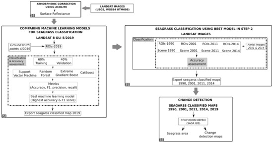
Figure 2.
Flowchart of image processing and change detection using Landsat images in Tauranga Harbour.
2.5.1. Atmospheric Correction
An atmospheric correction for all Landsat scenes was conducted using ACOLITE, in the PythonTM environment (Table A1, Appendix A) [52]. The original pixel values in physical digital number were converted to surface reflectance. Atmospheric corrected surface reflectance for pixels (limited by the study boundary, Figure 1) for the ρBlue (ρw482), the ρGeen (ρw561), and the ρRed (ρw654) bands were retained for all Landsat scenes in the years 1990, 2001, 2011, 2014, and 2019 for further processing steps. In the years 2014 and 2019, when Landsat 8 images were available, the coastal aerosol band (ρw443) was used, together with the ρBlue, ρGeen, and ρRed bands. The selected bands were used as independent variables in ML model prediction of the presence/absence of seagrass.
Due to inconsistency between the tidal status and the acquisition time of Landsat images, our study site was considered to contain both exposed and submerged areas. Therefore, the near infrared (ρNIR) band, which attenuates rapidly in water, was not used in the analysis. A water column correction was not employed for water pixels in Tauranga Harbour, since the water depth and water optical characteristics (i.e., attenuation coefficient of the solar radiance in the water column) were unavailable for the historic scenes (1990, 2001, 2011).
2.5.2. Application of Machine-Learning Algorithms
Hyper-Parameter Tuning for Selected Machine-Learning Models
Machine-learning models comprise several hyperparameters (i.e., the parameters that control the learning process during the implementation of ML models), which often need to be optimized (i.e., by the process of tuning) to find the best combination to achieve best classification performance. The hyper-parameters of the RF, the SVM, the XGB, and the CB models were tuned using a grid search with threefold cross-validation in the scikit-learn library [53]. The hyperparameters for each of the models were maintained during the training and the testing phases (Table A2, Appendix A).
Theoretical Background of the Machine-Learning Algorithms Used Random Forests
Random Forests (RF) [54] is perhaps the most popular machine-learning model for both classification and regression problems in remote sensing [55]. It is an ensemble bagging method, which uses a bootstrap sampling approach to build the training and the testing data and a voting method to select the most accurate decision from a large group of input decision tress. The RF model is a nonparametric method that is insensitive to the data’s distribution, reducing the overfitting. The RF technique supplies various hyperparameters for tuning; however, the large number of parameters in the model results in slow optimization.
Support Vector Machine
Support Vector Machine (SVM) [56,57] supports linear, poly-nominal, and radial basis function (RBF) kernels and can be adapted to various linear or non-linear data types. It has relatively few tunable hyperparameters but performance speed is still relatively slow when dealing with a large dataset. The SVM model uses a hyperplane to find the separation space among the classes with the most typical rules being: (i) better segregation of data; (ii) maximization of the distance between the closest data points and the hyperplane. Despite an accurate prediction and robustness to outliers, the SVM technique is not effective on overlaid classes or noisy datasets.
Extreme Gradient Boost
Extreme Gradient Boost (XGB) [17] is different from Gradient Boosting as it uses a more regularized model, which reduces over-fitting and results in a higher prediction accuracy. In the regularized gradient boosting mode, a selection of L1 or L2 regularization can be made to adapt the model to suit input data. Similar to other boosting models, the XGB technique supports various hyperparameters that are tuned using a grid search or genetic algorithm (GA) [58].
CatBoost
CatBoost (CB) was introduced in 2018 [59] for classification, regression, and ranking tasks. It can handle both category and numerical data types. Using ordered boosting on decision trees, a permutation-driven derivation from classic boosting, the CB yields a fast and reliable performance, even with a small dataset. The model itself produces robust predictive results with default hyperparameters, reducing the requirement of tuning, and its novel gradient boosting scheme results in less overfitting.
2.5.3. Comparison of ML Algorithms for Seagrass Mapping Using the Landsat Image Taken in 2019
Four ML models, SVM, RF, XGB, CB, were compared for seagrass mapping using the Landsat image from May 2019 and near-synchronous GTPs collected in April 2019 to identify the regions of interest (hereafter referred to as ROIs-2019) known to either seagrass or non-seagrass classes. The 1-month gap between the acquisition date of the Landsat image and the field survey date is acceptable due to the stable condition of the weather (i.e., no extreme weather phenomena) [60], and seagrass dynamics are slow in the study site [44,45]. A dataset of pixel reflectance values was extracted from ROIs-2019 and its corresponding Landsat image (dataset DS5, Table A3, Appendix A), split randomly into 60% for the training and 40% for the testing of selected ML models. The best model was selected as the model with highest accuracy and F1 score.
2.5.4. Seagrass Mapping Using Landsat Images in 1990, 2001, 2011, and 2014
The best ML model identified using the 2019 data was applied for mapping of seagrass using Landsat images from 1990, 2001, 2011, and 2014 (see Table 1 for date acquisition and spatial resolution of satellite images). The hyper-parameters developed using the 2019 data were retained for subsequent analysis, while the year-specific model was developed using ROIs containing seagrass and non-seagrass classes from the relevant year. For the years 2011 and 2014, we created these ROIs using aerial imagery [61] (hereafter referred to as ROIs-2011 and ROIs-2014). For 1990 and 2001, we used Google Earth images cross-referenced with the aerial images acquired between 1991 and 1992 (for creating ROIs-1990) and 2003 (for creating ROIs-2001). A dataset of pixel reflectance values was extracted from corresponding Landsat images (dataset DS1, DS2, DS3, and DS4, Table A3, Appendix A) for ROIs-1990, ROIs-2001, ROIs-2011, and ROIs-2014. Datasets were split randomly into 60% for training of the classification and 40% for the accuracy assessment for 1990, 2001, 2011, and 2014.
2.5.5. Change Detection
Change detection was conducted using the standard confusion matrix tool in the SAGA GIS [62]. The confusion matrix analyzed the changes of the pairs of classified maps (years 1990–2011 and 1990–2019), reporting in the map as seagrass loss (seagrass to non-seagrass), seagrass recovery (non-seagrass to seagrass), and unchanging seagrass.
2.6. Evaluation Criteria
We employed standard metrics for the evaluation of the classification skill: accuracy, Kappa coefficient (κ), Kendall’s tau coefficient (τ), precision, recall, and F1 (Equations (1)–(6)). These were applied independently to the five datasets listed in Table A3, to yield the skill of the initial model based on GTPs from DS5 (2019), and to check its performance when applied to the historic Landsat data in DS1 (1990), DS2 (2001), DS3 (2011), and DS4 (2014). Kendall’s tau coefficient was calculated using the SciPy library [63].
in which:
- ypred: predicted value
- y: corresponding true value
- po is the observed agreement
- pe is the expected agreement
- P: the number of concordant pair
- Q: the number of discordant pair
- U: the number of ties in predicted value
- T: the number of ties in true value
- tp: true positive
- fp: false positive
- fn: false negative
In addition, the nonparametric McNemar test was used to assess the statistical significance of the differences of the overall accuracy of the selected models in this research. The test was executed in a Python™ environment using the mlxtend library [64]. The chi-square value (χ2) was calculated from Equation (7) with Edward’s continuity correction.
in which:
- fn: false negative
- fp: false positive
3. Results
3.1. Performance of the RF, SVM, XGB, and CB Models Using Landsat Image and GTPs for 2019 Data
Of the four machine-learning models applied to the 2019 data, the CB model outperformed all others, with the F1 score, κ and τ coefficients reaching 0.95 (Table 3), and 0.92 (Table A4, Appendix A), respectively. The difference between models was statistically significant (McNemar’s test, Table 4) with the exception of the XGB and RF models. The CB model required a longer computation time (3.71 s) than the RF model (0.33 s), the XGB model (0.15 s), and the SVM model (0.04 s). The RF and XGB techniques showed an equivalent performance (Table 3) with F1 score of 0.93, while the SVM model underperformed the other models with a F1 score of 0.91.
Table 3.
Model performance for seagrass detection in Tauranga Harbour for the 2019 dataset.
Table 4.
Model performance comparison using McNemar’s test.
All models tested were able to classify seagrass from other bottom types in the harbor with a precision exceeding 0.89, but the highest precision was again from the CB model. Despite a similar F1 score, the XGB model gained a higher precision than the RF technique.
3.2. Seagrass Change Detection from 1990–2019
The CB technique was then used to make classification maps for the years 1990, 2001, 2011, and 2014 (Figure 3). Our results indicated a performance across all metrics that was equivalent to that in the 2019 case, with accuracy and F1 scores over 95% for the binary classification of seagrass and nonseagrass (Table 5 and Table A4, Appendix A).
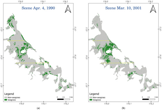
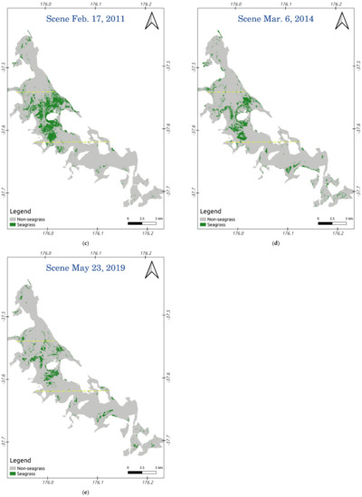
Figure 3.
Seagrass distribution in the years 1990, 2001, 2011, 2014, and 2019 (a–e) using the CB model (yellow lines indicate the boundaries of the northern, central, and southern harbor).
Table 5.
Accuracy assessment of the classified map using Landsat images in 1990, 2001, 2011, and 2014.
The time series shows that the seagrass meadow area decreased from 2237 ha in 1990 to 1184 ha in 2019, though not monotonically (Figure 3 and Figure 4). A downward trend from 1990 (2237 ha) to 2001 (2035 ha), was followed by a recovery in 2011 (to 2380 ha), followed by a second decline to 1184 ha in 2019 (Figure 4a). Different trends, though all with an overall decline to 2019, were discovered in the northern (Figure 4b), the central (Figure 4c), and the southern (Figure 4d) harbor. Seagrass attained the largest area in the central harbor, where it reached the peak of 1985 ha in 2011; however, it declined to 776 ha in 2019. In the northern harbor, seagrass was very abundant in 1990 with 549 ha, but strongly decreased to only 92 ha in 2001. This number increased to 242 ha in 2014 before suffered a second decline to 148 ha in 2019. Seagrass loss was also recorded in the southern harbor, at a slower rate of degradation, dropping from 576 ha in 1990 to 222 ha in 2011, and around 260 ha in 2019. Across the entire harbor, the recovery in 2011 was due to a large increase of seagrass areas from 2001 in the northern and the central harbors.
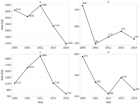
Figure 4.
Seagrass area in Tauranga Harbour from 1990–2019 derived from Landsat imagery with the variation in: (a) entire harbor; (b) northern harbor; (c) central harbor; (d) southern harbor.
The distribution of seagrass has also changed over time. In 1990, the meadows were similarly abundant in the northern, central, and southern harbors. Declines to 2001 mostly reflected losses from the northern and southern meadows, while the central meadows remained and were responsible for most of the expansion between 2001 and 2011 (Figure 3 and Figure 5). After 2011, there was no detectable recovery of the northern or the southern meadows, and the renewed overall decline was due to degradation of the central meadows, declining in area and becoming patchier by 2019 (Figure 3 and Figure 5).
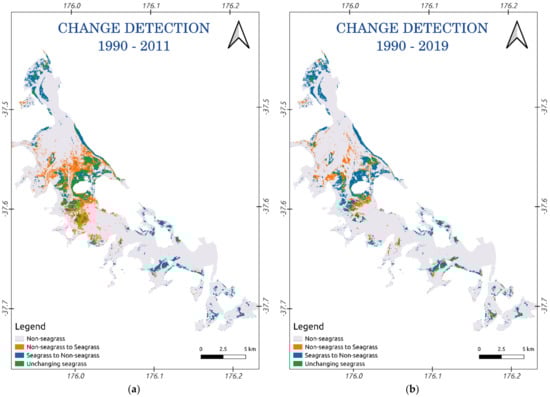
Figure 5.
Seagrass change detection between 1990–2011 (a) and 1990–2019 (b).
4. Discussion
In this investigation, we have demonstrated the use of machine-learning approaches successfully to classify seagrass in Landsat images of Tauranga Harbour, and to use this classification to detect changes in seagrass cover over a period of 29 years. Due to the relative paucity of field validation data from most of the time series of this analysis, we only tested a binary classification (seagrass and non-seagrass classes), but the four machine-learning models, RF, XGB, SVM, and CB, were all capable of detecting seagrass from other bottom types with high precision and recall scores. Previously, the RF and the SVM models have been tested for seagrass classification [65] and the RF for seagrass change detection in the Mediterranean [13]. These previous attempts have produced accuracies from 76–98% for Posidonia oceania [13,65] and 32–62% for Cymodocea nodosa using higher resolution RapidEye imagery [13], both lower than were achieved in this study using the CB technique. P. oceania and C. nodosa are structurally similar to Z. muelleri and would seem likely to offer a similar target. This suggests that the use of the state-of-the-art ML models with optimized hyper-parameters is an important factor contributing to the high-precision classification of seagrass presence/absence. Both the XGB and the CB techniques have been proven as potential candidates for a range of classification [58,66,67,68], and regression [69,70,71] problems but have not previously been applied to seagrasses, or to any other semi-submerged targets, so it is not clear if this is a general performance advantage in this type of application.
Other advantages over previous studies may, however, exist in Tauranga Harbour. Specifically, Z. muelleri occurs as monospecific meadows, without a substantial presence of macroalgae, which can degrade classifications [20,37], and where the reflectance value of seagrass is considerably different from the other common bottom types (sand, muddy sand, deep water). In addition, we were able to use cloud-free Landsat scenes, with atmospheric correction using ACOLITE, which has been designed for the aquatic application of Landsat imagery, which likely reduced the uncertainty of atmospheric impact and derived a higher quality of corrected surface reflectance [72].
In this study, the two boosting techniques (XGB, CB) and the one bagging (RF) outperformed the more traditional SVM methods. The SVM model does not work well with noisy data, where unclear margins exist between classes [73]. Such fuzzy margins were observed at the study site at the overlap between seagrass and non-seagrass (sand, muddy sand) classes, where the distinction between present and absent was gradual. This likely resulted in the relatively poor performance of the SVM model. The boosting techniques XGB (0.93) and CB (0.94) show slightly higher precision than the bagging RF (0.92), which might have resulted from the advancement in decision-tree growth of the boosting techniques. Unlike the RF model, which builds the independent decision tree from the bootstrapped samples, the boosting XGB and CB models sequentially grow new trees using the residual information of previous trees, which allows the new learner to solve the errors of the previous tree by minimizing the residual of the next model fitting. For a final prediction of a classification task, the bagging RF takes a majority vote from all decision trees while a weighted majority vote is adapted to the boosting techniques, such as XGB and CB, and potentially results in a higher precision of a class prediction.
Given the classification skill metrics, the CB is the best candidate for the mapping and change detection of seagrass in the study site. The CB is also amongst the latest emerging algorithms developed in the computer vision and pattern recognition fields (released in 2018); is easy to tune with fewer hyperparameters than the RF and the XGB techniques; and is using symmetric trees, which potentially results in faster optimization and prediction [59]. The CB model differs from the boosting algorithm family by using ordered boosting on a random permutation of given dataset, which prevent the prediction shift and alleviate the overfitting in model prediction. The outperformance of the CB over other ML models has been reported for mangrove total carbon estimation [74], various testing datasets [59], and forest aboveground biomass [75], which confirm the reliability and the capability of the CB implementation for seagrass mapping in our study. Our accurate long-term (29-year) change detection of seagrass meadows using the CB machine-learning model in Tauranga Harbour is a significant advance in the classification and monitoring of seagrass ecosystem using multispectral, remotely sensed data.
Our analysis has confirmed a general declining trend of seagrass cover in Tauranga Harbour reported previously [37] using aerial photography. In absolute terms, Park (2011) reported 2744 ha in March 2011, close to our estimate of 2380 ha at that time. Also, like Park, our analysis was able to resolve areas within the estuary where the greatest loss has occurred between assessments. We specifically noted that the seagrass loss was initially focused in the northern and southern parts of the harbor. High flux of sediment was recorded into the northern part, due to agricultural intensification, and the southern part, due to urban development, particularly after 2011 [47] and may explain the long-term decline of seagrass in those areas. The potential impact of agricultural and urban developments in the northern and the southern parts is supported by the observation that recovery was only observed in the central part of the harbor (Figure 3, year 2011, and Figure 5). Another potential factor contributing to long-term loss of seagrass is the grazing of black swans, which has previously been linked to variations in seagrass cover in the southern harbor [37,76]. Further analysis is required to develop a detailed explanation on the dynamics of seagrass meadows in Tauranga Harbour.
Here, we advocate the use of novel and advanced ML models, in combination with multitemporal Landsat images to obtain a long-term, historic series of observations on seagrass dynamics that will continue to be supported into the future through ongoing developments of the Landsat series. The proposed method potentially provides a low-cost, high-precision classification tool that can be extended to other estuaries with similar target conditions. While aerial photography and very high spatial resolution (VHR) satellite images have higher spatial resolution than Landsat images, they come at a high cost, and spatial coverage can be limited. Currently, Landsat is the most suitable satellite image resource for any long-term change detection due to its long time in service. A 30 m spatial resolution was found suitable to support a binary classification of seagrass in this study, and accuracy was unaffected by the small changes in spectral information that have accompanied the incremental changes in Landsat optical sensors. The most recent generation Landsat 8, with an improvement in radiometric resolution up to 16 bit (in the level 1 product), compared to the 8 bit in previous generations, and the addition of a coastal aerosol band, has good potential for accurate detection of the dynamics of seagrass. An improvement of spectral and radiometric resolution in Landsat 9 (scheduled for launching in 2021) is expected to provide continuity into the future monitoring of seagrass [77]. For a short-term observation of seagrass change, our proposed methods for seagrass classification are also potentially applicable to a wide range of VHR images (Quickbird, Ikonos, Unmanned Aerial Vehicle (UAV)) with consideration of the trade-off among the spatial coverage of the study site, the spatial resolution of the image, and the available budget.
The open-source approach is another significant advantage of our proposed methodology. The Python environment provides an excellent option for the end users to apply the novel machine-learning algorithms and remote-sensing data processing platform to support accurate mapping and estimation of the blue carbon budget of seagrass ecosystem [78]. Most commercial software only provides a limited number of processing and classification algorithms, with few, older ML options (e.g., SVM) and has a high license cost. Our proposed methods are more flexible, free of charge, and offer a high efficiency for mapping the dynamics of seagrass meadows in the complex coastal marine environment.
Despite a successful application of the CB model for seagrass classification and change detection, this research still comes with limitations. Since we used a supervised classification technique, both classification and validation require an independent assessment of seagrass cover in at least part of the remote image, to provide the ROIs that allow the training and validation steps. In addition, the seasonal growth of seagrass in temperate waters, and its intertidal habit, raise the uncertainty of change detection between various time points unless imagery is available at the same time, and under similar tidal conditions. The offset between Landsat, the time of image acquisition, and tidal regime (Table 1) is unavoidable in the study site; however, we consider that it is unlikely to significantly impact on classification accuracy. In Tauranga Harbour, seagrass meadows are distributed in the intertidal regions at a water depth ranging from 0 m (exposed) to a maximum of 1.5 m (at high tide) [37,51]. The ρBlue, ρGreen, and ρRed bands have nominal maximum penetration depths of 15, 10, 5 m respectively [34], and while moderate, but variable, coastal turbidity in the harbor will increase attenuation rate, the maximum immersion depth of 1.5 m suggests that the spectral bands reflectance signatures are highly likely to have been impacted by seagrass. Average vertical attenuation rate of the downwelling radiation within the 400–700 nm band in Tauranga Harbour is 0.40 m−1 (range 0.16–0.98 m−1) [79] and these authors found that 65% of incident radiation reached the estuary floor at 1.2 m depth. Again, this suggests that water clarity is sufficient to ensure that, even at maximum water depth, seagrass will contribute to the reflectance spectrum detected by the satellite. As with all satellite-based remote sensing, a cloud-free view is required, which constrains use of this technology.
To compensate for the limitation, we attempted to select all Landsat images acquired in the growing season of seagrass in Tauranga Harbour (austral summer and autumn) and at low tide, but this further constrains the availability of verifiable Landsat imagery for seagrass cover estimation. Further research focusing on expanding the novel approach used in the current study for long-term change detection of seagrass meadows is underway.
5. Conclusions
In this research, we used the novel machine-learning model CatBoost (CB) and other well-known ML models (RF, SVM, and XGB) for seagrass cover classification (present/absent), using Landsat satellite imagery, in Tauranga Harbour, New Zealand. Our results showed a high level of accuracy for all approaches, but the CB model outperformed the other selected models, with precision, recall, and F1 scores of 0.94, 0.96, and 0.95 respectively.
We then applied the CB technique to multispectral Landsat data for the detection of change in seagrass cover over a 29-year period between 1990 and 2019 in Tauranga Harbour. The change detection analysis determined an overarching declining trend of seagrass cover in Tauranga Harbour with approximately 50% loss over the 29 years period (from 2237 ha in 1990 to 1184 ha in 2019); these results concurred with a study using aerial imaging. Seagrass was lost in the far northern and southern areas of the harbor during the first part of this time, then more gradually from the central region. This analysis of change using Landsat images combined with the CB model demonstrates the value of historic satellite imagery and machine-learning for accurate documentation of the change over time in this difficult-to-quantify coastal vegetation.
Author Contributions
Conceptualization, Nam-Thang Ha and Ian Hawes; methodology, Nam-Thang Ha; software, Nam-Thang Ha; validation, Nam-Thang Ha and Tien-Dat Pham; resources, Nam-Thang Ha, Ian Hawes, Merilyn Manley-Harris; writing—original draft preparation, Nam-Thang Ha; writing—review and editing, Nam-Thang Ha, Tien-Dat Pham, Merilyn Manley-Harris, and Ian Hawes; supervision, Ian Hawes. All authors have read and agreed to the published version of the manuscript.
Funding
This research received no external funding.
Institutional Review Board Statement
Not applicable.
Informed Consent Statement
Not applicable.
Data Availability Statement
Data/material are available on request from the authors: The data and material that support the findings of this study are available from the corresponding author, Nam Thang Ha, upon reasonable request.
Acknowledgments
We are grateful for the support from Christine E. C. Gunfield and Matthew J. Finnigan from the Marine Field Station, Tauranga, New Zealand for the field survey.
Conflicts of Interest
The authors declare no conflict of interest.
Appendix A
Table A1.
Selected parameters for atmospheric correction using ACOLITE.
Table A1.
Selected parameters for atmospheric correction using ACOLITE.
| Parameter | Value |
|---|---|
| Ancillary data | |
| Gas transmittance | True |
| Ozone concentration (cm−1) | 0.3 |
| Water vapor concentration (g cm−2) | 1.5 |
| Pressure | Normal pressure |
| Masking | |
| Negative reflectance masking | True |
| Cirrus masking | True |
| Other parameters | |
| Sky correction | True |
| Dark spectrum fitting | Fixed |
| Sun glint correction | False |
| Output parameter | |
| Surface reflectance for water pixel (ρw) | ρw443 ρw482 ρw561 ρw654 |
Table A2.
The tuned hyperparameters of the RF, the SVM, the XGB, and the CB models.
Table A2.
The tuned hyperparameters of the RF, the SVM, the XGB, and the CB models.
| Random Forest | Extreme Gradient Boost | ||
|---|---|---|---|
| Bootstrap | True | Booster | GbTree |
| Max. depth | 8 | Gamma | 1 |
| Max. features | Auto | Learning rate | 0.2 |
| Min. sample leaf | 1 | Max. depth | 5 |
| Min. sample split | 3 | Min. child weight | 3 |
| Number of trees | 100 | Number of trees | 100 |
| Support Vector Machine | CatBoost | ||
| Kernel | RBF | Depth | 7 |
| C | 100 | Iteration (Number of trees) | 200 |
| Gamma | 1000 | Learning rate | 0.2 |
| L2 leaf reg | 1 | ||
Table A3.
Number of pixels for the training and the testing sets at various acquisition dates.
Table A3.
Number of pixels for the training and the testing sets at various acquisition dates.
| Dataset | Landsat Acquisition Date | Number of Pixels | |
|---|---|---|---|
| 60% for Training | 40% For Testing | ||
| DS1 | 4 April 1990 | 2171 | 1448 |
| DS2 | 10 March 2001 | 3000 | 2001 |
| DS3 | 17 February 2011 | 2618 | 1746 |
| DS4 | 6 March 2014 | 2544 | 1696 |
| DS5 | 23 May 2019 | 1830 | 1221 |
Table A4.
Kappa and Kendall’s tau coefficients of the classification.
Table A4.
Kappa and Kendall’s tau coefficients of the classification.
| Model | κ | τ | p-Value of τ |
|---|---|---|---|
| Data DS5, date 23 May 2019 | |||
| RF | 0.90 | 0.90 | 0.00 |
| SVC | 0.87 | 0.87 | 0.00 |
| CB | 0.92 | 0.92 | 0.00 |
| XGB | 0.90 | 0.90 | 0.00 |
| Data DS1, date 4 April 1990 | |||
| CB | 0.95 | 0.95 | 0.00 |
| Data DS2, date 10 March 2001 | |||
| CB | 0.92 | 0.92 | 0.00 |
| Data DS2, date 17 February 2011 | |||
| CB | 0.94 | 0.94 | 0.00 |
| Data DS4, date 6 March 2014 | |||
| CB | 0.93 | 0.93 | 0.00 |
Table A5.
List of acronyms and abbreviations.
Table A5.
List of acronyms and abbreviations.
| Acronym/Abbreviation | Meaning | Explanation |
|---|---|---|
| ACOLITE | Atmospheric correction for operational land imager (OLI) ‘lite’ toolbox | A Python language-based application for atmospheric correction of satellite imagery |
| Accuracy | An agreement degree between the classified values and the ground-truth values in a classification task | |
| CB | CatBoost | A machine-learning algorithm |
| XGB | Extreme Gradient Boost | A machine-learning algorithm |
| F1 | F1 | A harmonic measurement of precision and recall scores in the prediction of a machine-learning model |
| GPS | Global Positioning System | A satellite-based system providing positioning services |
| GTPs | Ground-Truth Points | GTPs are the boundary points of any given classes in the study site, defined by GPS |
| Κ | Kappa coefficient | A statistical index measuring the accuracy (agreement between predictions and ground-truthed values) of the classification. A higher Kappa coefficient denotes a more accurate classification |
| τ | Kendall’s tau coefficient | A nonparametric measurement to evaluate the classification’s accuracy. A higher Kendall’s tau coefficient denotes a more accurate classification |
| ML | Machine learning | An artificial intelligence (AI) approach that builds an application/algorithm for a specific output by learning from data |
| NIR | Near infrared | The near infrared region in the electromagnetic spectrum |
| Precision | A score to measure the success of the prediction of a machine-learning model. A higher precision denotes a more accurate prediction | |
| RF | Random Forest | A machine-learning algorithm |
| Recall | A score to measure the success of the prediction of a machine-learning model. A higher recall denotes a more accurate prediction | |
| RBF | Radial basis function | A function used in the Support Vector Machine model, together with linear and polynomial functions |
| ROI | Region of interest | A bounded region used in image classification where the pixels contain a given class |
| SVM | Support Vector Machine | A machine-learning algorithm |
| UAV | Unmanned aerial vehicle | An aircraft without a human pilot |
| GLOVIS | USGS Global Visualization Viewer | A web-based system for satellite image visualization and downloading |
| UTM | Universal Transverse Mercator | A map projection |
| VHR | Very high spatial resolution | Indicating satellite images that have spatial resolution from centimeters to a few meters |
| WGS | World Geodetic System | A standard coordinate system used in cartography. |
References
- Nordlund, L.M.; Jackson, E.L.; Nakaoka, M.; Samper-Villarreal, J.; Beca-Carretero, P.; Creed, J.C. Seagrass Ecosystem Services—What’s Next? Mar. Pollut. Bull. 2018, 134, 145–151. [Google Scholar] [CrossRef]
- Nordlund, L.M.; Koch, E.W.; Barbier, E.B.; Creed, J.C. Seagrass Ecosystem Services and Their Variability across Genera and Geographical Regions. PLoS ONE 2016, 11, e0163091. [Google Scholar] [CrossRef] [PubMed]
- Fourqurean, J.W.; Duarte, C.M.; Kennedy, H.; Marbà, N.; Holmer, M.; Mateo, M.A.; Apostolaki, E.T.; Kendrick, G.A.; Krause-Jensen, D.; McGlathery, K.J.; et al. Seagrass Ecosystems as a Globally Significant Carbon Stock. Nat. Geosci. 2012, 5, 505–509. [Google Scholar] [CrossRef]
- Gullström, M.; Lyimo, L.D.; Dahl, M.; Samuelsson, G.S.; Eggertsen, M.; Anderberg, E.; Rasmusson, L.M.; Linderholm, H.W.; Knudby, A.; Bandeira, S.; et al. Blue Carbon Storage in Tropical Seagrass Meadows Relates to Carbonate Stock Dynamics, Plant–Sediment Processes, and Landscape Context: Insights from the Western Indian Ocean. Ecosystems 2018, 21, 551–566. [Google Scholar] [CrossRef]
- Orth, R.J.; Carruthers, T.J.B.; Dennison, W.C.; Duarte, C.M.; Fourqurean, J.W.; Heck, K.L.; Hughes, A.R.; Kendrick, G.A.; Kenworthy, W.J.; Olyarnik, S.; et al. A Global Crisis for Seagrass Ecosystems. BioScience 2006, 56, 987. [Google Scholar] [CrossRef]
- Waycott, M.; Duarte, C.M.; Carruthers, T.J.B.; Orth, R.J.; Dennison, W.C.; Olyarnik, S.; Calladine, A.; Fourqurean, J.W.; Heck, K.L.; Hughes, A.R.; et al. Accelerating Loss of Seagrasses across the Globe Threatens Coastal Ecosystems. Proc. Natl. Acad. Sci. USA 2009, 106, 12377–12381. [Google Scholar] [CrossRef] [PubMed]
- Marbà, N.; Arias-Ortiz, A.; Masqué, P.; Kendrick, G.A.; Mazarrasa, I.; Bastyan, G.R.; Garcia-Orellana, J.; Duarte, C.M. Impact of Seagrass Loss and Subsequent Revegetation on Carbon Sequestration and Stocks. J. Ecol. 2015, 103, 296–302. [Google Scholar] [CrossRef]
- Cullen-Unsworth, L.; Unsworth, R. Seagrass Meadows, Ecosystem Services, and Sustainability. Environ. Sci. Policy Sustain. Dev. 2013, 55, 14–28. [Google Scholar] [CrossRef]
- Hejnowicz, A.P.; Kennedy, H.; Rudd, M.A.; Huxham, M.R. Harnessing the Climate Mitigation, Conservation and Poverty Alleviation Potential of Seagrasses: Prospects for Developing Blue Carbon Initiatives and Payment for Ecosystem Service Programmes. Front. Mar. Sci. 2015, 2. [Google Scholar] [CrossRef]
- Bujang, J.S.; Zakaria, M.H.; Short, F.T. Seagrass in Malaysia: Issues and Challenges Ahead. In The Wetland Book; Finlayson, C.M., Milton, G.R., Prentice, R.C., Davidson, N.C., Eds.; Springer: Dordrecht, The Netherlands, 2018; pp. 1875–1883. ISBN 978-94-007-4000-6. [Google Scholar]
- Unsworth, R.K.F.; McKenzie, L.J.; Collier, C.J.; Cullen-Unsworth, L.C.; Duarte, C.M.; Eklöf, J.S.; Jarvis, J.C.; Jones, B.L.; Nordlund, L.M. Global Challenges for Seagrass Conservation. Ambio 2018. [Google Scholar] [CrossRef]
- Pham, D.; Yokoya, N.; Bui, D.; Yoshino, K.; Friess, D. Remote Sensing Approaches for Monitoring Mangrove Species, Structure, and Biomass: Opportunities and Challenges. Remote Sens. 2019, 11, 230. [Google Scholar] [CrossRef]
- Traganos, D.; Reinartz, P. Interannual Change Detection of Mediterranean Seagrasses Using RapidEye Image Time Series. Front. Plant Sci. 2018, 9. [Google Scholar] [CrossRef] [PubMed]
- Paulose, N.E.; Dilipan, E.; Thangaradjou, T. Integrating Indian Remote Sensing Multi-Spectral Satellite and Field Data to Estimate Seagrass Cover Change in the Andaman and Nicobar Islands, India. Ocean Sci. J. 2013, 48, 173–181. [Google Scholar] [CrossRef]
- Roelfsema, C.; Lyons, M.; Dunbabin, M.; Kovacs, E.M.; Phinn, S. Integrating Field Survey Data with Satellite Image Data to Improve Shallow Water Seagrass Maps: The Role of AUV and Snorkeller Surveys? Remote Sens. Lett. 2015, 6, 135–144. [Google Scholar] [CrossRef]
- Hossain, M.S.; Bujang, J.S.; Zakaria, M.H.; Hashim, M. The Application of Remote Sensing to Seagrass Ecosystems: An Overview and Future Research Prospects. Int. J. Remote Sens. 2015, 36, 61–114. [Google Scholar] [CrossRef]
- Chen, C.-F.; Lau, V.-K.; Chang, N.-B.; Son, N.-T.; Tong, P.-H.-S.; Chiang, S.-H. Multi-Temporal Change Detection of Seagrass Beds Using Integrated Landsat TM/ETM+/OLI Imageries in Cam Ranh Bay, Vietnam. Ecol. Inform. 2016, 35, 43–54. [Google Scholar] [CrossRef]
- Amone-Mabuto, M.; Bandeira, S.; da Silva, A. Long-Term Changes in Seagrass Coverage and Potential Links to Climate-Related Factors: The Case of Inhambane Bay, Southern Mozambique. West. Indian Ocean J. Mar. Sci. 2017, 16, 13–25. [Google Scholar]
- Phinn, S.R.; Kovacs, E.M.; Roelfsema, C.M.; Canto, R.F.; Collier, C.J.; McKenzie, L.J. Assessing the Potential for Satellite Image Monitoring of Seagrass Thermal Dynamics: For Inter- and Shallow Sub-Tidal Seagrasses in the Inshore Great Barrier Reef World Heritage Area, Australia. Int. J. Digit. Earth 2018, 11, 803–824. [Google Scholar] [CrossRef]
- Ha, N.T.; Manley-Harris, M.; Pham, T.D.; Hawes, I. A Comparative Assessment of Ensemble-Based Machine Learning and Maximum Likelihood Methods for Mapping Seagrass Using Sentinel-2 Imagery in Tauranga Harbor, New Zealand. Remote Sens. 2020, 12, 355. [Google Scholar] [CrossRef]
- McCarthy, M.J.; Halls, J.N. Habitat Mapping and Change Assessment of Coastal Environments: An Examination of WorldView-2, QuickBird, and IKONOS Satellite Imagery and Airborne LiDAR for Mapping Barrier Island Habitats. ISPRS Int. J. Geo-Inf. 2014, 3, 297–325. [Google Scholar] [CrossRef]
- Sousa, L.P.; Sousa, A.I.; Alves, F.L.; Lillebø, A.I. Ecosystem Services Provided by a Complex Coastal Region: Challenges of Classification and Mapping. Sci. Rep. 2016, 6, 22782. [Google Scholar] [CrossRef]
- Camps-Valls, G. Machine Learning in Remote Sensing Data Processing. In Proceedings of the 2009 IEEE International Workshop on Machine Learning for Signal Processing, Grenoble, France, 1–4 September 2009; pp. 1–6. [Google Scholar]
- Lary, D.J.; Alavi, A.H.; Gandomi, A.H.; Walker, A.L. Machine Learning in Geosciences and Remote Sensing. Geosci. Front. 2016, 7, 3–10. [Google Scholar] [CrossRef]
- Maxwell, A.E.; Warner, T.A.; Fang, F. Implementation of Machine-Learning Classification in Remote Sensing: An Applied Review. Int. J. Remote Sens. 2018, 39, 2784–2817. [Google Scholar] [CrossRef]
- Ahmad, H. Machine learning applications in oceanography. Aquat. Res. 2019, 161–169. [Google Scholar] [CrossRef]
- Machova, K.; Puszta, M.; Barcak, F.; Bednar, P. A Comparison of the Bagging and the Boosting Methods Using the Decision Trees Classifiers. Comput. Sci. Inf. Syst. 2006, 3, 57–72. [Google Scholar] [CrossRef]
- Bühlmann, P. Bagging, Boosting and Ensemble Methods. In Handbook of Computational Statistics; Gentle, J.E., Härdle, W.K., Mori, Y., Eds.; Springer: Berlin/Heidelberg, Germany, 2012; pp. 985–1022. ISBN 978-3-642-21550-6. [Google Scholar]
- Huettmann, F. Boosting, Bagging and Ensembles in the Real World: An Overview, some Explanations and a Practical Synthesis for Holistic Global Wildlife Conservation Applications Based on Machine Learning with Decision Trees. In Machine Learning for Ecology and Sustainable Natural Resource Management; Springer International Publishing: Berlin/Heidelberg, Germany, 2018; pp. 63–83. [Google Scholar]
- Yaman, E.; Subasi, A. Comparison of Bagging and Boosting Ensemble Machine Learning Methods for Automated EMG Signal Classification. Available online: https://www.hindawi.com/journals/bmri/2019/9152506/ (accessed on 2 December 2020).
- Northrop, A. IDEAS—LANDSAT Products Description Document; USGS: Reston, VA, USA, 2015; p. 68.
- Zhu, Z. Change Detection Using Landsat Time Series: A Review of Frequencies, Preprocessing, Algorithms, and Applications. ISPRS J. Photogramm. Remote Sens. 2017, 130, 370–384. [Google Scholar] [CrossRef]
- Ihlen, V. Landsat 8 (L8) Data Users Handbook; USGS: Reston, VA, USA, 2019.
- Green, E.P.; Mumby, P.J.; Edwards, A.J.; Clark, C.D. A Review of Remote Sensing for the Assessment and Management of Tropical Coastal Resources. Coast. Manag. 1996, 24, 1–40. [Google Scholar] [CrossRef]
- Ha, N.T.; Yoshino, K.; Hoang Son, T.P. Seagrass Mapping Using ALOS AVNIR-2 Data in Lap An Lagoon, Thua Thien Hue, Viet Nam; Frouin, R.J., Ebuchi, N., Pan, D., Saino, T., Eds.; SPIE: Kyoto, Japan, 2012; p. 85250S. [Google Scholar]
- Garcia, R.; Hedley, J.; Tin, H.; Fearns, P. A Method to Analyze the Potential of Optical Remote Sensing for Benthic Habitat Mapping. Remote Sens. 2015, 7, 13157–13189. [Google Scholar] [CrossRef]
- Park, S.G. Extent of Seagrass in the Bay of Plenty in 2011; Environmental Publication; Bay of Plenty Reginal Council: Whakatane, New Zealand, 2011; p. 52.
- Reeve, G.; Stephens, S.; Wadhwa, A. Tauranga Harbour Inundation Modelling; NIWA: Tauranga, New Zealand, 2018; p. 107. [Google Scholar]
- Tay, H.; Bryan, K.; de Lange, W.; Pilditch, C. The Hydrodynamics of the Southern Basin of Tauranga Harbour. N. Z. J. Mar. Freshw. Res. 2013, 47, 249–274. [Google Scholar] [CrossRef]
- Collier, C.J.; Villacorta-Rath, C.; van Dijk, K.; Takahashi, M.; Waycott, M. Seagrass Proliferation Precedes Mortality during Hypo-Salinity Events: A Stress-Induced Morphometric Response. PLoS ONE 2014, 9, e94014. [Google Scholar] [CrossRef] [PubMed]
- York, P.H.; Gruber, R.K.; Hill, R.; Ralph, P.J.; Booth, D.J.; Macreadie, P.I. Physiological and Morphological Responses of the Temperate Seagrass Zostera Muelleri to Multiple Stressors: Investigating the Interactive Effects of Light and Temperature. PLoS ONE 2013, 8, e76377. [Google Scholar] [CrossRef] [PubMed]
- Collier, C.J.; Ow, Y.X.; Langlois, L.; Uthicke, S.; Johansson, C.L.; O’Brien, K.R.; Hrebien, V.; Adams, M.P. Optimum Temperatures for Net Primary Productivity of Three Tropical Seagrass Species. Front. Plant Sci. 2017, 8. [Google Scholar] [CrossRef] [PubMed]
- Turner, S.J. Growth and Productivity of Intertidal Zostera Capricorni in New Zealand Estuaries. N. Z. J. Mar. Freshw. Res. 2007, 41, 77–90. [Google Scholar] [CrossRef]
- Ramage, D.L.; Schiel, D.R. Reproduction in the Seagrass Zostera Novazelandica on Intertidal Platforms in Southern New Zealand. Mar. Biol. 1998, 130, 479–489. [Google Scholar] [CrossRef]
- Schwarz, A.-M.; Turner, S. Management and Conservation of Seagrass in New Zealand: An Introduction; Science & Technical Publishing: Wellington, New Zealand, 2006; p. 90. [Google Scholar]
- Hicks, M.; Semadeni-Davies, A.; Haddadchi, A.; Shankar, U.; Plew, D. Updated Sediment Load Estimator for New Zealand; NIWA Client Report 2018341CH prepared for Ministry for the Environment; National Institute of Water and Atmospheric Research Ltd.: Christchurch, New Zealand, 2019; p. 190. [Google Scholar]
- Hicks, M. Review and Analysis of Suspended Sediment Monitoring in the Tauranga Moana Catchment; NIWA Client Report 2019183CH prepared for Bay of Plenty Regional Council; NIWA: Auckland, New Zealand, 2019; p. 57. [Google Scholar]
- Cabaço, S.; Santos, R.; Duarte, C.M. The Impact of Sediment Burial and Erosion on Seagrasses: A Review. Estuar. Coast. Shelf Sci. 2008, 79, 354–366. [Google Scholar] [CrossRef]
- Saunders, M.I.; Atkinson, S.; Klein, C.J.; Weber, T.; Possingham, H.P. Increased Sediment Loads Cause Non-Linear Decreases in Seagrass Suitable Habitat Extent. PLoS ONE 2017, 12, e0187284. [Google Scholar] [CrossRef]
- USGS GloVis. Available online: https://glovis.usgs.gov/ (accessed on 2 February 2019).
- Park, S.G. Changes in Abundance of Seagrass (Zostera spp.) in Tauranga Harbour from 1959–1996; Environment BOP: Whakatane, New Zealand, 1999; p. 19.
- RBINS. ACOLITE Python User Manual; RBINS: Brussels, Belgium, 2018; p. 10. [Google Scholar]
- Pedregosa, F.; Varoquaux, G.; Gramfort, A.; Michel, V.; Thirion, B.; Grisel, O.; Blondel, M.; Prettenhofer, P.; Weiss, R.; Dubourg, V.; et al. Scikit-Learn: Machine Learning in Python. J. Mach. Learn. Res. 2011, 12, 2825–2830. [Google Scholar]
- Breiman, L. Random Forest. Mach. Learn. 2001, 45, 5–32. [Google Scholar] [CrossRef]
- Belgiu, M.; Drăguţ, L. Random Forest in Remote Sensing: A Review of Applications and Future Directions. ISPRS J. Photogramm. Remote Sens. 2016, 114, 24–31. [Google Scholar] [CrossRef]
- Mountrakis, G.; Im, J.; Ogole, C. Support Vector Machines in Remote Sensing: A Review. ISPRS J. Photogramm. Remote Sens. 2011, 66, 247–259. [Google Scholar] [CrossRef]
- Tomar, D.; Agarwal, S. Twin Support Vector Machine: A Review from 2007 to 2014. Egypt. Inform. J. 2015, 16, 55–69. [Google Scholar] [CrossRef]
- Georganos, S.; Grippa, T.; Vanhuysse, S.; Lennert, M.; Shimoni, M.; Wolff, E. Very High Resolution Object-Based Land Use–Land Cover Urban Classification Using Extreme Gradient Boosting. IEEE Geosci. Remote Sens. Lett. 2018, 15, 607–611. [Google Scholar] [CrossRef]
- Prokhorenkova, L.; Gusev, G.; Vorobev, A.; Dorogush, A.V.; Gulin, A. CatBoost: Unbiased Boosting with Categorical Features. arXiv 2019, arXiv:170609516. [Google Scholar]
- NIWA. The National Climate Database. Available online: https://cliflo.niwa.co.nz/ (accessed on 20 July 2020).
- BOPRC Seagrass Extent—Bay of Plenty. Available online: http://gis.boplass.govt.nz/arcgis/rest/services/imagery (accessed on 20 October 2019).
- Conrad, O.; Bechtel, B.; Bock, M.; Dietrich, H.; Fischer, E.; Gerlitz, L.; Wehberg, J.; Wichmann, V.; Böhner, J. System for Automated Geoscientific Analyses (SAGA) v. 2.1.4. Geosci. Model Dev. 2015, 8, 1991–2007. [Google Scholar] [CrossRef]
- Virtanen, P.; Gommers, R.; Oliphant, T.E.; Haberland, M.; Reddy, T.; Cournapeau, D.; Burovski, E.; Peterson, P.; Weckesser, W.; Bright, J.; et al. SciPy 1.0: Fundamental Algorithms for Scientific Computing in Python. Nat. Methods 2020, 17, 261–272. [Google Scholar] [CrossRef] [PubMed]
- Raschka, S. MLxtend: Providing Machine Learning and Data Science Utilities and Extensions to Python’s Scientific Computing Stack. J. Open Source Softw. 2018, 3, 638. [Google Scholar] [CrossRef]
- Traganos, D.; Reinartz, P. Mapping Mediterranean Seagrasses with Sentinel-2 Imagery. Mar. Pollut. Bull. 2017. [Google Scholar] [CrossRef]
- Sun, F.; Wang, R.; Wan, B.; Su, Y.; Guo, Q.; Huang, Y.; Wu, X. Efficiency of Extreme Gradient Boosting for Imbalanced Land Cover Classification Using an Extended Margin and Disagreement Performance. ISPRS Int. J. Geo-Inf. 2019, 8, 315. [Google Scholar] [CrossRef]
- Pham, T.D.; Le, N.N.; Ha, N.T.; Nguyen, L.V.; Xia, J.; Yokoya, N.; To, T.T.; Trinh, H.X.; Kieu, L.Q.; Takeuchi, W. Estimating Mangrove Above-Ground Biomass Using Extreme Gradient Boosting Decision Trees Algorithm with Fused Sentinel-2 and ALOS-2 PALSAR-2 Data in Can Gio Biosphere Reserve, Vietnam. Remote Sens. 2020, 12, 777. [Google Scholar] [CrossRef]
- Pham, T.D.; Yokoya, N.; Xia, J.; Ha, N.T.; Le, N.N.; Nguyen, T.T.T.; Dao, T.H.; Vu, T.T.P.; Pham, T.D.; Takeuchi, W. Comparison of Machine Learning Methods for Estimating Mangrove Above-Ground Biomass Using Multiple Source Remote Sensing Data in the Red River Delta Biosphere Reserve, Vietnam. Remote Sens. 2020, 12, 1334. [Google Scholar] [CrossRef]
- Lou, I.; Xie, Z.; Ung, W.K.; Mok, K.M. Freshwater Algal Bloom Prediction by Extreme Learning Machine in Macau Storage Reservoirs. Neural Comput. Appl. 2016, 27, 19–26. [Google Scholar] [CrossRef]
- Maier, P.M.; Keller, S. Machine Learning Regression on Hyperspectral Data to Estimate Multiple Water Parameters. In Proceedings of the 2018 9th Workshop on Hyperspectral Image and Signal Processing: Evolution in Remote Sensing (WHISPERS), Amsterdam, The Netherlands, 23–26 September 2018; IEEE: Amsterdam, The Netherlands, September 2018; pp. 1–5. [Google Scholar]
- Lee, Y.; Han, D.; Ahn, M.-H.; Im, J.; Lee, S.J. Retrieval of Total Precipitable Water from Himawari-8 AHI Data: A Comparison of Random Forest, Extreme Gradient Boosting, and Deep Neural Network. Remote Sens. 2019, 11, 1741. [Google Scholar] [CrossRef]
- Vanhellemont, Q. Adaptation of the Dark Spectrum Fitting Atmospheric Correction for Aquatic Applications of the Landsat and Sentinel-2 Archives. Remote Sens. Environ. 2019, 225, 175–192. [Google Scholar] [CrossRef]
- Karamizadeh, S.; Abdullah, S.M.; Halimi, M.; Shayan, J.; Rajabi, M.j. Advantage and Drawback of Support Vector Machine Functionality. In Proceedings of the 2014 International Conference on Computer, Communications, and Control Technology (I4CT), Langkawi, Malaysia, 2–4 September 2014; IEEE: Langkawi, Malaysia, 2014; pp. 63–65. [Google Scholar]
- Pham, T.D.; Yokoya, N.; Nguyen, T.T.T.; Le, N.N.; Ha, N.T.; Xia, J.; Takeuchi, W.; Pham, T.D. Improvement of Mangrove Soil Carbon Stocks Estimation in North Vietnam Using Sentinel-2 Data and Machine Learning Approach. GISci. Remote Sens. 2020, 58, 1–20. [Google Scholar] [CrossRef]
- Luo, M.; Wang, Y.; Xie, Y.; Zhou, L.; Qiao, J.; Qiu, S.; Sun, Y. Combination of Feature Selection and CatBoost for Prediction: The First Application to the Estimation of Aboveground Biomass. Forests 2021, 12, 216. [Google Scholar] [CrossRef]
- Dos Santos, V.M.; Matheson, F.E.; Pilditch, C.A.; Elger, A. Is Black Swan Grazing a Threat to Seagrass? Indications from an Observational Study in New Zealand. Aquat. Bot. 2012, 100, 41–50. [Google Scholar] [CrossRef]
- USGS Landsat 9. Available online: Https://Www.Usgs.Gov/Land-Resources/Nli/Landsat/Landsat-9 (accessed on 20 November 2019).
- Macreadie, P.I.; Anton, A.; Raven, J.A.; Beaumont, N.; Connolly, R.M.; Friess, D.A.; Kelleway, J.J.; Kennedy, H.; Kuwae, T.; Lavery, P.S.; et al. The Future of Blue Carbon Science. Nat. Commun. 2019, 10, 3998. [Google Scholar] [CrossRef] [PubMed]
- Cussioli, M.C.; Bryan, K.R.; Pilditch, C.A.; de Lange, W.P.; Bischof, K. Light Penetration in a Temperate Meso-Tidal Lagoon: Implications for Seagrass Growth and Dredging in Tauranga Harbour, New Zealand. Ocean Coast. Manag. 2019, 174, 25–37. [Google Scholar] [CrossRef]


Publisher’s Note: MDPI stays neutral with regard to jurisdictional claims in published maps and institutional affiliations. |
© 2021 by the authors. Licensee MDPI, Basel, Switzerland. This article is an open access article distributed under the terms and conditions of the Creative Commons Attribution (CC BY) license (https://creativecommons.org/licenses/by/4.0/).