Abstract
Analysis of urban land use dynamics is essential for assessing ecosystem functionalities and climate change impacts. The focus of this study is on monitoring the characteristics of urban expansion in Hang-Jia-Hu and evaluating its influences on forests by applying 30-m multispectral Landsat data and a machine learning algorithm. Firstly, remote sensed images were preprocessed with radiation calibration, atmospheric correction and topographic correction. Then, the C5.0 decision tree was used to establish classification trees and then applied to make land use maps. Finally, spatiotemporal changes were analyzed through dynamic degree and land use transfer matrix. In addition, average land use transfer probability matrix (ATPM) was utilized for the prediction of land use area in the next 20 years. The results show that: (1) C5.0 decision tree performed with precise accuracy in land use classification, with an average total accuracy and kappa coefficient of more than 90.04% and 0.87. (2) During the last 20 years, land use in Hang-Jia-Hu has changed extensively. Urban area expanded from 5.84% in 1995 to 21.32% in 2015, which has brought about enormous impacts on cultivated land, with 198,854 hectares becoming urban, followed by forests with 19,823 hectares. (3) Land use area prediction based on the ATPM revealed that urbanization will continue to expand at the expense of cultivated land, but the impact on the forests will be greater than the past two decades. Rationality of urban land structure distribution is important for economic and social development. Therefore, remotely sensed technology combined with machine learning algorithms is of great significance to the dynamic detection of resources in the process of urbanization.
1. Introduction
Since the reform and opening up of China in the late 1970s, urbanization in China has attracted worldwide attention. The proportion of urban population has increased from 18% in 1978 to 50% in 2010 and is projected to increase to 60% by 2020 and 80% or more by 2030 [1,2]. Urbanization has become one of the themes of development in most countries in the world and is the most important factor of driving land use cover change (LUCC) [3,4]. This not only means the promotion of rapid economic development, but also an increase in building density, reduced green space and increased urban disasters caused by extreme weather [5,6]. Urban area accounts for less than 3% of the global land surface, but 90% of the world’s economy, 50% of the world’s population, 60% of energy consumption and 70% of greenhouse gas emissions come from cities [7]. Therefore, urbanization management is especially important and land use dynamic monitoring is the most direct manifestation of it.
Land use change occurs every year due to the interaction of natural conditions and human activities, and it is one of the major driving forces of global change [8,9]. Since the huge influence on ecosystem functions including ecosystem biodiversity and carbon sinks, the dynamics of land use patterns have always been the focus of research related to LUCC. Recently, the reduction of forest area due to LUCC caused by urbanization has had a greater impact on global carbon sequestration capacity [10,11]. According to relevant research, the area occupied by forest ecosystems is only 27.6% of the global area, but about 57% of the world’s carbon is fixed by forest ecosystems [12]. Forest resources are the largest carbon pool in terrestrial ecosystems and play an irreplaceable role in regulating global carbon balance and mitigating climate change [13,14]. Therefore, dynamic monitoring of changes in forest resources is increasingly important for mitigating the global warming.
Land use change detection can quickly extract land information and update land use maps by observing the state of objects during different periods [15,16]. Maps of LUCC can quantify a wide range of processes such as forest harvesting, forest disturbances, land use pressures and urban expansion, which are all important for rational use and scientific management of land resources [17,18]. Traditional field surveys can accurately evaluate the development trends and characteristics of LUCC, but field surveys require a large amount of manpower, material resources, financial resources, and time, which is impractical for large-scale monitoring of dynamic changes in land use [19]. With the development of remote sensing technology, satellite remote sensing has been widely used to detect LUCC [20,21]. The specialty of large-scale and real-time monitoring give remotely sensed observations salient merits in detection of LUCC and are gradually becoming the most effective means in this field [22,23]. Methods of dynamic land use monitoring can be divided into two categories: direct spectral comparison and post-classification comparison [24]. Direct spectral comparison analyzes images pixel by pixel, which has limits in the interpretation of land information in different periods. Post-classification comparison directly contrasts the pre- and post-classification results, and thus can obtain spatiotemporal information for different land types [25]. Since the accuracy of classification can directly influence the analysis results, the selection of classification methods is becoming an important part of dynamic change research [26,27].
Classification methods such as K-Nearest Neighbor, support vector machine, and the maximum likelihood method, due to the interpretable output results, the amount of large calculation work, and the weak correlation analysis between attributes, are rarely used in precise classification studies. As a core technology in the field of artificial intelligence research, machine learning is widely used in computer graphics, recommendation systems, software engineering, and bioinformatics [28,29,30]. Machine learning can train and experience data according to the large amount of information provided by the datasets and simultaneously optimizes its own algorithm rules [31,32], which has attracted much attention in improving the accuracy of image classification in recent years. Currently, common machine learning classification algorithms include deep learning neural networks and decision trees. Deep learning in classification requires a large number of parameters, such as the weights, and the thresholds; the learning process cannot be observed, and the output is difficult to interpret [33]. Decision tree theory [34,35] has previously been used to classify remote sensing dataset and offers some advantages over other classification methods [36,37]. Visual rules of decision tree in the classification process allow users to alter the range of the node threshold in accordance with the target need and then extract the terrestrial information more accurately. The C5.0 decision tree is a new algorithm developed from the original ID3 [38]. It uses the boosting method to generate a series of decision trees to determine the best classification variables and optimal segmentation points through information gain ratio (Info Gain Ratio). For image data with different resolutions, C5.0 decision tree can improve the classification accuracy to a large extent. Cui et al. [39] proposed a method of extracting national bamboo forest information based on decision tree combined with mixed pixel decomposition by using MODIS reflectivity product and the classification accuracy was more than 80% at different times. Funkenberg et al. [40] used C5.0 algorithm to detect dynamic change of grassland in Mekong by using Landsat images showed that area converted from grassland to other land types due to natural disasters in 1991 was 77%. Lv et al. [41] used images from the GeoEye-1 satellite with a resolution of 0.5 m to study automatic identification methods for farmland forest networks, showing that the accuracy of the automatic recognition was above 92% and the average accuracy was 92.97%.
Hang-Jia-Hu is located in the Yangtze River Delta in Zhejiang province [42,43]. As a region of rapid economic evolution, urbanization has become the main and most crucial driving force in LUCC during this rapid economic development. This paper aims to use Landsat time series data, applying a post-classification comparison method based on C5.0 decision tree to analyze spatial changes of urban expansion in Hang-Jia-Hu during the past 20 years. In addition, the impact of urban expansion on forest is then evaluated. Finally, the tendency of land use change in the next 20 years is predicted by applying the development law of land use change over the past 20 years.
2. Study Area and Datasets
2.1. Study Area
Hang-Jia-Hu region is located in the northern part of Zhejiang Province in China (Figure 1), ranging from 118°50’15’’ E to 121°19’6’’E and from 29°42’52’’ N to 31°11’53’’ N. Its climate is subtropical monsoon, and annual average temperature is 15~18 °C with an average annual precipitation of about 1100 mm. The study area is about 1.476 million hectares including Jiaxing, the majority of Huzhou and the northeastern part of Hangzhou. Specific regions include Linan (LN), Yuhang (YH), Jiaxing (JX), Jiashan (Js), Anji (AJ), Fuyang (FY), Pinghu (PH), Deqing (DQ), Hangzhou (HangZ), Tongxiang (TX), Hanning (HN), Haiyan (HY), Huzhou (HuZ), Xioashan (XS) and Changxing (CX). Forests in this place are mainly distributed in the southwest, and the main forest types are broadleaf forest (BLF), coniferous forest (CNF), and bamboo forest (BMF).
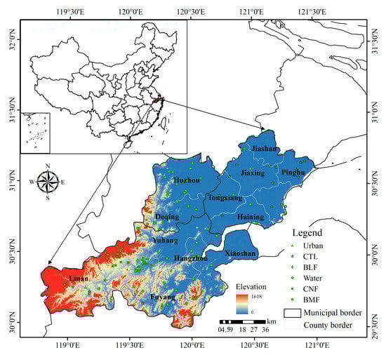
Figure 1.
Study area and ground survey plots of 2015.
2.2. Datasets and Processing
Satellite 30-m multispectral data of Landsat5 TM (1995, 2000, 2005, 2009) and Landsat8 OLI (2015) were downloaded from the United States Geological Survey (USGS, http://glovis.usgs.gov/). We selected cloud-free images from the years with ground observations for 3 scenes that cover our study area (Table 1). Due to the overall poor image quality of study area in 2010, we decided to use the images in 2009 to correspond with field data in 2010.

Table 1.
Acquisition date of the image datasets.
Remote sensed data is easily influenced by water vapor, aerosol, bidirectional reflection and data transmission, which can result in serious fluctuations of time series data and influence the desired effect in data analysis [44,45]. Therefore, this study applied Fast Line-of-sight Atmospheric Analysis of Spectral Hypercubes (FLAASH) [46,47] to correct each image for the purpose of eliminating the part of the effect caused by the atmosphere. Since the terrain may affect the brightness values of original imagery, a digital elevation model (DEM) was used to make terrain correction for pixel values. In addition, terrain correction data was downloaded from the Geospatial Data Cloud website (http://www.gscloud.cn/).
According to the original “Technical Regulations for Inventory for Forest Management Planning and Design” of the former Ministry of Forestry in 1996 and the “Technical Operation Rules for Forest Management Planning and Design in Zhejiang Province” in 1997, the land use types of this study were determined as BMF, BLF, CNF, cultivated land (CTL), water, and urban (including buildings and roads) [48,49]. Field observation of classification verification plots of BMF, BLF and CNF were derived from the data of National Forest Inventory (NFI) in Zhejiang province. The investigation method of NFI is systematic sampling, which is usually evenly placed at the intersection of kilometer grids of 1:50,000 topographic maps. Each plot size is 28.5 m × 28.5 m [50]. Verification plots of other land use types were obtained from field investigation and image visual interpretation. Specific verification number of different land use types are shown in Table 2.
Table 2.
Number of verification plots in different years.
3. Study Methodology
3.1. C5.0 Decision Tree
Decision tree is a typical supervised classification method of machine learning algorithm [51,52]. It generates a decision tree or rules in line with inductive learning of training data and then uses them to classify remotely sensed images. Decision tree models require no assumptions about data distribution and can process high-dimensional data sets quickly [53,54]. C5.0 decision tree [55] is a binary tree structure formed by cyclic analysis of the training dataset composed of feature attributes and target variables. It consists of a root node, a series of branches and a final node and is classified by the ultimate node.
Information Gain (Info Gain) [56] is defined in information theory as the difference between the entropy of a dataset to be classified and the conditional entropy of a selected feature. It is an indicator used to select features in a decision tree algorithm. The larger Info Gain is, the better selectivity of this feature is. Info Gain Ratio [57] is also called the information gain rate and is calculated by Info Gain and information entropy of the feature. C5.0 decision tree calculates the Info Gain Ratio of all features, and some of them with relatively high value in distinguishing land types will be selected as the tested variables of operational nodes to divide dataset. Then, pruning and merging nodes can make balanced of accuracy and complexity of decision tree. Finally, optimal classification rules by constructing the best multi-branched tree structure is used to classify images of the study area. The decision tree generated is easy to interpret without requiring a large amount of training time to establish [58,59].
3.2. Construction of the Decision Tree
Decision tree construction usually includes selection of variables, decision tree generation, and pruning of the decision tree [60]. Variables selection is a process of calculating Info Gain Ratio of all variables and choosing optimal variables with high values as the segmentation to divide datasets. Branches will be pruned when the weighted error of node is beyond its father node. Then, an optimal decision tree is generated. This study used the See5.0 classifier coupled with ENVI classic 5.0 to construct the decision tree [61]. The amount of training data in each land use type was set to be the same (800 pixels) so as to reduce the deviation of classifier system. Despite the visible classification rules of the C5.0 algorithm, observing the classification results when modifying the node threshold of decision tree or optimizing the training data can improve the accuracy of analysis. Considering different land use types will show different spectrum and texture information from season to season, so we decided to construct a corresponding classification decision tree for images in different periods, whereby separate classifications can make classification results more accurate and reliable.
It is obvious that the characteristics of the remotely sensed image will greatly depend on the spectra in the classification. In addition to the original image bands, the first three principal components (PC_1, PC_2, PC_3) [62] by component analysis and vegetation indices—normalized vegetation index (NDVI), enhanced vegetation index (EVI), SAVI (Soil Adjusted Vegetation Index) and improved normalized difference water index (MNDWI)—were extracted by using band operation and were all set as input variables in the classification (Table 3).
Table 3.
Remote sensing variables of land use classification.
3.3. Evalution of Urban Expansion
One indicator of dynamic change in evaluating urbanization is dynamic degree [65]. This refers to the amplitude of change of urban area during a given period of time, and it can intuitively reveal the speed of change of a number of pixels in urban areas [66,67]. The formula is calculated as follows:
In Equation (1): K is the dynamic degree of urban area change, and refers to the average annual rate of urban area change. Ua and Ub are the area of the urban cover at the beginning and the end of the period, respectively. T is the time interval of the study. When K is greater than 0, it indicates that the area of urban cover shows an expanding trend. Otherwise, it represents a decreasing trend.
Contribution rate (P) refers to the contribution rate of other land use types to urban change [68]. This paper uses the land use transfer matrix to calculate P.
In Equations (2), Pi is the contribution rate of a given land use type to urban growth; Mi is the area of a given land use type that has been converted into urban use; i is the land use type, i = 1, 2, 3, 4, 5.
3.4. Land Use Prediction
The land use transfer matrix is an important representation for describing and measuring changes in LUCC [69]. It can provide us with the source and composition of land use type transfer in the initial and final stages of research, which is an important way of studying the temporal and spatial evolution of LUCC [70]. In this study, the land use transfer matrix was employed to calculate P and ATPM. Then, we used ATPM to compute the land use area in 2000, 2005, 2009 and 2015, which is defined as the predicted area, and compared the predicted results with the classified area based on the C5.0 algorithm. The determination coefficient R2 and RMSE (Root Mean Square Error) between the predicted area and the classified area of land use were used to explain the fitness of the ATPM with respect to prediction. The high R2 and small RMSE mean the ATPM has a good effect on predicting the area of land use, and it could be applied to predicting the area of different land use areas in 2020, 2025, 2030 and 2035. R2 and RMSE are calculated as follows:
In Equations (3) and (4), R2 and RMSE are indicators of simulation accuracy; oi is the classified area of land types in a given year; pi is the predicted area of land use calculated by the average land use transfer probability matrix multiplied by the classified area in the previous year; is the average classified area of different land types in a given year.
4. Results and Analysis
4.1. Classification Decision Trees
The a, b, c, d and e in Figure 2 respectively represent the optimal classification decision tree in 1995, 2000, 2005, 2009 and 2015.
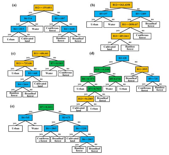
Figure 2.
Optimal decision trees of image classification from 1995 to 2015 (a–e).
The various optimal decision trees indicate that there is a big difference among the variables and nodes threshold of segmentation in different years. Overall, the original bands are most of the variables used to build the decision tree, and the structure of the variables used by each tree varies greatly. Although images are processed to a uniform atmospheric correction, the difference in the time of image acquisition still have some effect, and there are also differences in the spectral image values of Landsat TM and Landsat OLI. Therefore, the values of the optimal characteristic bands selected when extracting forest information will be different. In Figure 2, with respect to vegetation, the original image bands and the first three components were mainly used to construct the rules from 1995 to 2009. In addition, B6 is the segmentation variable for discriminating the three forest types. B4, B5 and B6 are mainly used to extract bamboo forest from the other two forest types, especially B4, which divides it and broadleaf forest in 1995 and 2005. However, B7 (NDVI) seems to be more important in the segmentation of land types in 2015. This is mainly because of the formation date of the different images. NDVI, as the standard index for monitoring the growth state of vegetation, is able to separate them from other land types, and the vegetation in 2015 is growing in maturity, exhibiting a high value. As for urban and water, B5 and B6 are the core segmentation variables, and are prominent from other bands with different thresholds in different years.
4.2. Classification Result and Verification Accuracy
The results of land use maps in Hang-Jia-Hu based on the application of the optimal decision trees are shown in Figure 3.
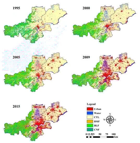
Figure 3.
Land use classification map from 1995 to 2015.
The accuracy of land use classification in 1995, 2000, 2005, 2009 and 2015 is shown in Table 4. In addition to the BMF with an average accuracy of 88.42%, the accuracy of other land uses in different years are all above 90%. The overall accuracies of different periods are all above 90%, with an average accuracy of 93.40%. Kappa coefficients are all above 0.88, which means that the classifications show precise results. This illustrates that the classification of land use using the C5.0 decision tree exhibits good performance.
Table 4.
Classification accuracy of land use types in different years.
4.3. Analysis of Urban Expansion
The urban area in Hang-Jia-Hu region changed considerably. The dynamic degree of urbanization and the average urban area from 1995 to 2015 in 13 districts are shown in Figure 4. The dynamics degree of different districts varied greatly. In most districts, after a small-scale reduction of urban area, there was a large expansion in the next stage. This may be because the demolition of urban areas and their subsequent reconstruction. During 2000 and 2005, the dynamics were larger than other stages, and were positive in all districts. Several districts with a relatively large urban dynamic degree were not major cities, but rather those with a smaller average urban area. This illustrates that expansion has a greater impact on districts with smaller urban areas. For example, HN, JS and TX have the relatively high dynamic of urban expansion that is beyond the amplitude in HangZ, JX and HZ. Moreover, even though there was a small decline in some districts in specific periods, there were still some where the urban area increased continuously. Dynamic degree in FY, HN, HangZ, JX, XS and YH were positive in the four periods, which means that the urban area in these districts was in a state of expansion.
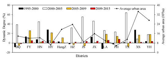
Figure 4.
Dynamic degree and average area of urban in 13 districts from 1995 to 2015.
Urban area has increased by 2.65 times in the past two decades. To clearly understand the changes of urban expansion in different regions, we created a spatial distribution map of urban expansion at different stages (Figure 5). Urban dynamic degree in Jiaxing City at 18.21% was the highest, followed by Hangzhou City at 13.62%. Urban expansion in Huzhou City was not greatly similar to the other two areas, and had the smallest value of urban dynamic at 7.2%. Evolution of spatial distribution of urban growth in different years varied from region to region. Urban growth in Jiaxing City seemed to expand from the urban center to the surrounding areas, especially in the main city of Jiaxing. In Hangzhou City, urbanization was concentrated in the urban core of HangZ and XS, and the direction of urban expansion was from the northeast to the southwest. Urban change in Huzhou City was distributed in the main city of HZ and DQ. Large-scale urban growth in DQ region mainly occurred in the stage from 2000 to 2005. The spatial distribution of urban changes in the main city of Hang-Jia-Hu are presented in the black frames marked A, B and C in Figure 5. We selected three city center areas in HangZ City, JX City and HZ City, with analysis window sizes of 58,871 hectares, 31,192 hectares and 16,317 hectares, respectively. The urban area in the main city of HangZ (Figure 5A) increased from 16,116.3 hectares to 36,607.6 hectares, representing a size increase of 2.27 times. Its growth was mainly in the northeast from 1995 to 2000 and in the northwest from 2005 to 2015. In addition to the first stage, urban growth was centralized in northwest in the following three stages, which indicated that urbanization in the core of HangZ City had a tendency of northwest expansion. Urban change omnidirectionally from the original central area to the surrounding area was the major characteristics of JX (Figure 5B). Urbanization was the most intense, with an area increment of 12,677.5 hectares, or 6.68 times. In addition, the expansion rate was the fastest in the stage from 2000 to 2005. In addition, the degree of expansion was much smaller than previously during the 2009 to 2015 stage. In the main city of HZ (Figure 5C), the urban expansion phenomenon seems the most moderate, with an area growth of 1.9 times. The expansion before 2005 was mainly concentrated around the center of the city. After 2005, it expanded to the north, the west and the northeast.
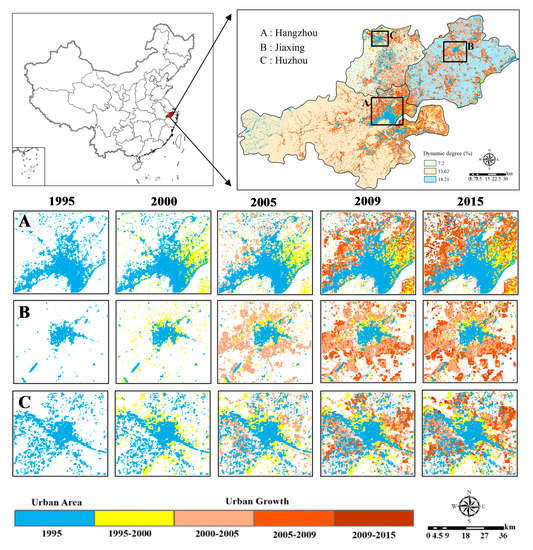
Figure 5.
Spatiotemporal distribution of urban growth in Hangzhou (A), Jiaxing (B) and Huzhou (C) from 1995 to 2015.
4.4. Impact of Urbanization on Forests
We analyzed the area change of land use in this study and its contribution to urban expansion (Figure 6). Based on the results, CTL, which is the main source of urban expansion, has led to a significant area loss over the last two decades. The trend of contribution rate to urban expansion decreased continuously (from 91.61% in the first stage to 82.23% in the final stage), but it remained the main source of urban expansion throughout the study period. BLF and BMF also showed an increasing trend in their contribution rate to urban area when it exhibited a small increase. The allocation of forest resources is always in dynamic balance. CNF, with the largest value, is the most likely source of urban expansion prior to 2009, but it also decreases in its contribution to the increase in urban area due to the decrease in area. In addition, BLF became the major source of expansion between 2009 and 2015. However, although the overall forest area decreased, its contribution rate to urban expansion gradually increased, which indicates that the probability of future urban expansion using BLF and BMF as sources of expansion will gradually increase. The changing factors of water bodies are more complicated. At the same time, due to the difficulty of transforming water bodies into urban areas, its area and the contribution rate to the increase in urban area has no obvious evolution to follow. Overall, the vegetation in this study observed strong laws regarding area and contribution rate to urban growth during the urbanization process. A sustained urban expansion with a certain land use type as a source of expansion will result in a significant decline in the land area. At the same time, this will also lead to a gradual decrease in the probability of becoming a source of expansion, thus exhibiting a reaction phenomenon in the process of urbanization.
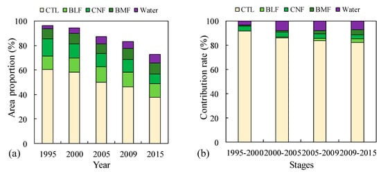
Figure 6.
Area proportion (a) and contribution rate to urban expansion (b) from 1995 to 2015.
According to the statistics, the total amount of forests lost due to urban expansion was 19,823 hectares, which accounts for 71.05% of the total decrease in forest. This illustrates that urbanization is the major factor leading to the decrease in forests. Figure 7 reflects the spatial distribution of forest areas changing into urban areas (Figure 7a) and the specific changes in different stages (Figure 7b).
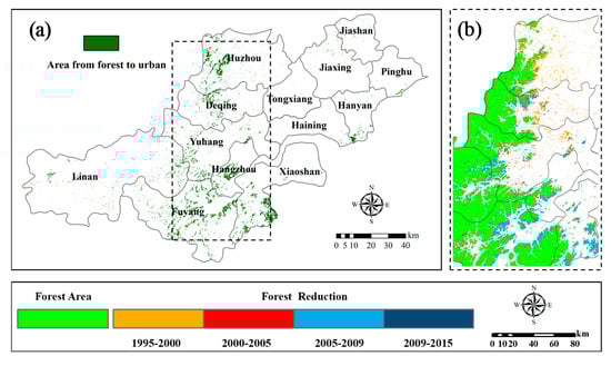
Figure 7.
(a) Changing distribution of area from forest to urban land use, (b) different stages of forest changes.
Forest reduction occurred mainly at the junction of urban and forest areas, which were mainly distributed in the central and western parts of HZ, DQ, HangZ, XS and FY. It is clear that the forest area gradually decreased from 1995 to 2015. The reduction from 1995 to 2000 is most obvious in the western part of HZ. In addition, the area loss was the most significant from 2005 to 2009, with a decline of 12.18%, which accounted for 43% of the total reduction in the study period. The declines in 2009 and 2015 were significantly less, which was also a result of the decrease of the contribution rate of forest to urban growth. The direction of forest area reduction was from northeast to southwest, which is consistent with the overall direction of urban expansion. Forest loss due to urbanization was centrally distributed in the southern part of HZ and FY. In particular, FY, which had the largest dynamic degree (above 24%) of urban expansion, accounted for the highest ratio of forest reduction, further indicating that urban expansion is synchronized with the reduction of forest in this region.
4.5. Prediction of LUCC for the Next 20 Years
We obtained the transition probability matrices of four periods through the land use transfer matrix and the land area of the four periods, and obtained the ATPM of the four probability matrices (Table 5). The ATPM was multiplied by the land areas of 1995, 2000, 2005, and 2009 to obtain the land areas of 2000, 2005, 2009, and 2015, and the results were compared with the classification areas of the corresponding years. Then, R2 and RMSE were used to observe the correlation and error between the predicted area and the classified area. The results are shown in Figure 8.
Table 5.
The ATPM of four probability matrices in four stages.
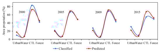
Figure 8.
Classified and predicted land use area proportion from 2000 to 2015.
The forests in Figure 8 and Figure 9 include BLF, CNF and BMF. The area proportion in Figure 8 shows that the predicted area has a strong relationship with the classified area. The R2 between the classified area and the predicted area in 2000, 2005, 2009 and 2015 are in the range of 0.94 and 0.99, with RMSE ranging from 1.61 × 10⁴ hm2 to 7.86 × 10⁴ hm2. This means that the predicted results displayed a precise accuracy, which further illustrated that the ATPM could perform well when predicting land area from 2000 to 2015 and could be applied in the prediction of area use for the next 20 years.
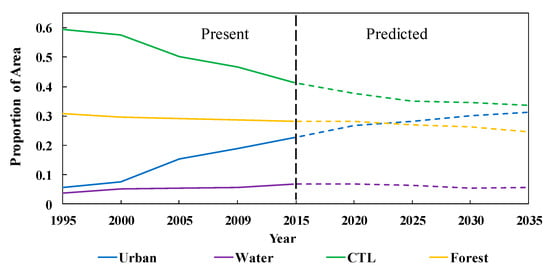
Figure 9.
Area proportion of land use area from 1995 to 2035.
Based on the ATPM, we calculated the land use area from 2020 to 2035 and drew the overall area trend for the land use dynamics of the previous 20 years and the next 20 years (Figure 9). According to the structure of land use from 1995 to 2015, urban expansion is accompanied by an intense reduction in CTL and a slight decline in forest area. In addition, based on the prediction results from 2020 to 2035, CTL will continue to decline, although the magnitude of change will be relatively lower than before. However, the phenomenon of forest reduction will be more obvious than in the previous 20 years, especially in 2030 and 2035. This shows that urbanization will continue to reduce CTL as a source of expansion in the next 20 years, but the impact on forests will gradually increase. With this pattern, and considering no other external economic and social factors, urban expansion will continue to occur, growing more serious and leading to the large-scale occupation of CTL, causing greater area loss of forest.
5. Discussion
We used remote sensing data combined with decision tree to analyze the spatiotemporal evolution of urban expansion in Hang-Jia-Hu and its impact on forests. In the process of using the C5.0 algorithm to establish classification rules, we found that the original band accounted for 51.7% of the variables involved in constructing the classification tree, while the vegetation index was only 20.7%. This shows that the vegetation index is not always the criterion used to distinguish between vegetation and non-vegetation in the classification process. At the same time, due to the uncertainty of the image spectral information, the optimal segmentation variables of different regions and different time periods also have large differences. The accuracy of land use maps is especially important for land use change analysis. The temporal mismatch between remote sensing and field survey data due to the lack of cloud-free Landsat scenes corresponding to the exact times of ground observation can lead to accuracy error in the verification results [19]. We used images from 2009 as a substitute for 2010, which caused error in the verification process. In addition, accuracy verification results of the land use maps showed that BFM was the major reason for the overall decrease in accuracy. This is because different impervious surfaces have similar spectral signatures, which can result in misclassification [71]. The spectral characteristics of BMF are close to those of BLF and CNF, resulting in a high degree of error in the process of manual visual interpretation and selection of training samples for the establishment of the decision tree. In addition, due to the significance of forests with respect to ecosystem functionalities, the effect of minor changes in forests on humans cannot be ignored. The analysis of urbanization in this study reveals that urbanization, mainly at the expense of CTL, also has a huge impact on forests. Therefore, accurate monitoring of forest changes is of great significance. In particular, forest loss in urban interior locations should attended to more closely. However, detection of urban forests based on remote sensing technology mainly uses hyperspectral and high-resolution data, because it is difficult to accurately detect subtle changes in low- and medium-resolution satellite data. Improving the time and spatial resolution of the datasets and the evaluation methods of urban research may improve the accuracy of measurements of urbanization. Finally, ATPM in this study represents the trend of the change in land use area in Hang-Jia-Hu during the last two decades, and it was used to predict the trend for the next 20 years with a certain degree of reliability. Furthermore, R2 and RMSE in the prediction results of the past 20 years also show that ATPM has higher accuracy in the prediction of land use area. However, the prediction results of this study can only represent the general situation of the land area change for the next 20 years under the current development trend, but not specific trends in future development. Since the overall trend of urban development on a large regional scale can be used by land resource managers in order to draw meaningful conclusions at a macro scale and implement rational planning, urban prediction is of great significance for urban planners and builders.
6. Conclusions
Based on the multitemporal Landsat imagery and the C5.0 decision tree, we analyzed the changes in urban expansion and their impact on forests in the Hang-Jia-Hu region. The results showed that using the C5.0 algorithm to establish decision trees for image data acquired in different years can reduce the terrestrial homologue phenomenon caused by different dates of image acquisition, which can greatly improve the extraction accuracy. During the past two decades, land use in Hang-Jia-Hu region has changed greatly. The urban area increased by 2.65 times (nearly 209,100 hectares) with respect to the original. JX City, with the largest dynamic degree of urban growth, expanded from the urban center to the surroundings, especially in the JX district. HangZ City, with an urban dynamic of 13.62%, gradually expanded westward. This phenomenon was more obvious in LA district and FY district. With the process of urbanization, the CTL area shows a significant decline, changing from covering an area from 60.37% in 1995 to and area of 37.58% in 2015, as a result of the massive occupation of urban expansion. In terms of the pace of CTL decline, its contribution rate to urban growth gradually decreased. The total area of BLF, CNF and BMF presented a small amplitude of reduction, but its contribution to urban expansion was incremental, which means that the probability of future urbanization using forests as a source of expansion will increase. Land use area prediction indicates that in the next 20 years, urban use will continue to expand at the expense of CTL, but this impact will become more tempered than in the past 20 years. On the contrary, forests will be affected more seriously in the future because of urban expansion.
Author Contributions
Conceptualization, Meng Zhang, Huaqiang Du and Guomo Zhou; Formal analysis, Meng Zhang, Huaqiang Du, Fangjie Mao and Xuejian Li; Funding acquisition, Huaqiang Du and Guomo Zhou; Investigation, Meng Zhang, Luofan Dong, Junlong Zheng, Di’en Zhu, Hua Liu, Zihao Huang and Shaobai He; Methodology, Meng Zhang, Huaqiang Du, Fangjie Mao and Xuejian Li; Project administration, Huaqiang Du and Guomo Zhou; Software, Meng Zhang, Huaqiang Du, Xuejian Li, Luofan Dong and Di’en Zhu; Validation, Meng Zhang and Fangjie Mao; Writing—original draft, Meng Zhang; Writing—review & editing, Meng Zhang, Huaqiang Du, Fangjie Mao and Guomo Zhou. All authors have read and agreed to the published version of the manuscript.
Funding
This study was undertaken with the support of the National Natural Science Foundation (No. U1809208,31670644), the State Key Laboratory of Subtropical Silviculture Foundation (No. zy20180201), the Joint Research fund of Department of Forestry of Zhejiang Province and Chinese Academy of Forestry (2017SY04), Zhejiang Provincial Collaborative Innovation Center for Bamboo Resources and High-efficiency Utilization (No. S2017011), the National Natural Science Foundation (No.31901310).
Acknowledgments
The authors would like to thank anonymous reviewers for their helpful comments and suggestions.
Conflicts of Interest
The authors declare no conflict of interest.
References
- Wheaton, W.C.; Shishido, H. Urban Concentration, Agglomeration Economies, and the Level of Economic Development. Econ. Dev. Cult. Chang. 1981, 30, 17–30. [Google Scholar] [CrossRef]
- Wu, J.; Chen, B.; Mao, J.; Feng, Z. Spatiotemporal evolution of carbon sequestration vulnerability and its relationship with urbanization in China’s coastal zone. Sci. Total Environ. 2018, 645, 692. [Google Scholar] [CrossRef] [PubMed]
- Zhou, C.; Wang, S.; Wang, J. Examining the influences of urbanization on carbon dioxide emissions in the Yangtze River Delta, China: Kuznets curve relationship. Sci. Total Environ. 2019, 675, 472–482. [Google Scholar] [CrossRef] [PubMed]
- Xu, Q.; Dong, Y.X.; Yang, R. Influence of land urbanization on carbon sequestration of urban vegetation: A temporal cooperativity analysis in Guangzhou as an example. Sci. Total Environ. 2018, 635, 26–34. [Google Scholar] [CrossRef]
- Goodchild, B. Homes, Cities and Neighbourhoods; Routledge: Abingdon, UK, 2008. [Google Scholar]
- Mahmoud, S.H.; Gan, T.Y. Urbanization and climate change implications in flood risk management: Developing an efficient decision support system for flood susceptibility mapping. Sci. Total Environ. 2018, 636, 152–167. [Google Scholar] [CrossRef]
- Güneralp, B.; Zhou, Y.; Ürge-Vorsatz, D.; Gupta, M.; Yu, S.; Patel, P.L.; Fragkias, M.; Li, X.; Seto, K.C. Global scenarios of urban density and its impacts on building energy use through 2050. Proc. Natl. Acad. Sci. USA 2017, 114, 8945. [Google Scholar] [CrossRef]
- Mao, J.X.; Li, Z.G.; Yan, X.P.; Zhou, S.H. The impact of landscape-urbanization upon land use change with microscopic data. Acta Ecol. Sin. 2008, 28, 3584–3596. [Google Scholar]
- Hao, H.M.; Ren, Z.Y. Land Use/Land Cover Change (LUCC) and Eco-Environment Response to LUCC in Farming-Pastoral Zone, China. Agric. Sci. China 2009, 8, 91–97. [Google Scholar] [CrossRef]
- Bing, L.I.; Jun, B.I.; Tian, Y. Analysis of LUCC and Driving Force in Heavy Polluted Area in Taihu Lake Basin. Environ. Sci. Technol. 2011, 5, 43–48. [Google Scholar]
- Schneider, A.; Logan, K.E.; Kucharik, C.J. Impacts of Urbanization on Ecosystem Goods and Services in the U.S. Corn Belt. Ecosystems 2012, 15, 519–541. [Google Scholar] [CrossRef]
- Reynolds, R.; Liang, L.; Li, X.C.; Dennis, J. Monitoring Annual Urban Changes in a Rapidly Growing Portion of Northwest Arkansas with a 20-Year Landsat Record. Remote Sens. 2017, 9, 71. [Google Scholar] [CrossRef]
- Giardina, C.P.; Coleman, M.; Binkley, D.; Hancock, J.; King, J.S.; Lilleskov, E.; Loya, W.M.; Pregitzer, K.S.; Ryan, M.G.; Trettin, C. The Response of Belowground Carbon Allocation in Forests to Global Change. Tree Species Effects on soils: Implications for Global Change; Kluwer Academic Publishers: Dordrecht, The Netherlands, 2005; pp. 119–154, Chapter 7. [Google Scholar]
- Berenguer, E.; Gardner, T.A.; Ferreira, J.; Aragão, L.E.O.C.; Camargo, P.B.; Cerri, C.E.; Durigan, M.; Junior, R.C.O.; Vieira, I.C.G.; Barlow, J. Developing Cost-Effective Field Assessments of Carbon Stocks in Human-Modified Tropical Forests. PLoS ONE 2015, 10, 3713–3726. [Google Scholar] [CrossRef] [PubMed]
- Schneider, A.; Friedl, M.A.; Potere, D. Mapping global urban areas using MODIS 500-m data: New methods and datasets based on ‘urban ecoregions’. Remote Sens. Environ. 2010, 114, 1733–1746. [Google Scholar] [CrossRef]
- Zhou, X.; Chen, H. Impact of urbanization-related land use land cover changes and urban morphology changes on the urban heat island phenomenon. Sci. Total Environ. 2018, 635, 1467–1476. [Google Scholar] [CrossRef] [PubMed]
- Jeon, S.B.; Olofsson, P.; Woodcock, C.E. Land use change in New England: A reversal of the forest transition. J. Land Use Sci. 2014, 9, 105–130. [Google Scholar] [CrossRef]
- Olofsson, P.; Foody, G.M.; Herold, M.; Stehman, S.V.; Woodcock, C.E.; Wulder, M.A. Good practices for estimating area and assessing accuracy of land change. Remote Sens. Environ. 2014, 148, 42–57. [Google Scholar] [CrossRef]
- Zhang, M.; Du, H.; Zhou, G.; Li, X.; Mao, F.; Dong, L.; Zheng, J.; Liu, H.; Huang, Z.; He, S. Estimating Forest Aboveground Carbon Storage in Hang-Jia-Hu Using Landsat TM/OLI Data and Random Forest Model. Forests 2019, 10, 1004. [Google Scholar] [CrossRef]
- Giraldo, M.A. Land-use and land-cover assessment for the study of lifestyle change in a rural Mexican community: The Maycoba Project. Int. J. Health Geogr. 2012, 11, 27. [Google Scholar] [CrossRef]
- Arifasihati, Y. Analysis of Land Use and Cover Changes in Ciliwung and Cisadane Watershed in three Decades. Procedia Environ. Sci. 2016, 33, 465–469. [Google Scholar] [CrossRef][Green Version]
- Wang, Y.; Liu, L.; Wang, Z. Land Covermapping based on Landsat Time-series Stacks in Sanjiang Plain. Remote Sens. Technol. Appl. 2015, 30, 959–968. [Google Scholar]
- Du, H.; Sun, X.; Han, N.; Mao, F. Comprehensive object-oriented and decision-making tree survey factors and remote sensing estimation of carbon stocks. J. Appl. Ecol. 2017, 28, 3163–3173. [Google Scholar]
- Bounoua, L.; Ping, Z.; Mostovoy, G.; Thome, K.; Masek, J.; Imhoff, M.; Shepherd, M.; Quattrochi, D.; Santanello, J.; Silva, J. Impact of urbanization on US surface climate. Environ. Res. Lett. 2015, 10, 084010. [Google Scholar] [CrossRef]
- Ding, J. Study on oasis water body themation extraction using PCA way. Yunnan Geogr. Environ. Res. 2005, 17, 11–14. [Google Scholar]
- Lu, M.; Xu, Y.; Shan, N.; Wang, Q.; Wang, J. Effect of urbanisation on extreme precipitation based on nonstationary models in the Yangtze River Delta metropolitan region. Sci. Total Environ. 2019, 673, 64–73. [Google Scholar] [CrossRef] [PubMed]
- Luan, C.; Dong, G. Experimental Identification of Hard Data Sets for Classification and Feature Selection Methods with Insights on Method Selection. Data Knowl. Eng. 2018, 118, 41–51. [Google Scholar] [CrossRef]
- Foster, K.R.; Koprowski, R.; Skufca, J.D. Machine learning, medical diagnosis, and biomedical engineering research-commentary. Biomed. Eng. Online 2014, 13, 94. [Google Scholar] [CrossRef]
- Kotsiantis, S.B. Supervised machine learning: A review of classification techniques. Emerg. Artif. Intell. Appl. Comput. Eng. 2007, 160, 3–24. [Google Scholar]
- Schleier-Smith, J. An Architecture for Agile Machine Learning in Real-Time Applications. In Proceedings of the 21th ACM SIGKDD International Conference on Knowledge Discovery and Data Mining (KDD’15), Sydney, Australia, 10–13 August 2015; pp. 2059–2068. [Google Scholar]
- Zaman, S.; Rifat, S.M.R. Performance Analysis of Supervised Machine Learning Algorithms for Text Classification. In Proceedings of the 19th International Conference on Computer and Information Technology (ICCIT), Dhaka, Bangladesh, 18–20 December 2016. [Google Scholar]
- Kinnings, S.L.; Liu, N.; Tonge, P.J.; Jackson, R.M.; Xie, L.; Bourne, P.E. Correction to “A Machine Learning-Based Method To Improve Docking Scoring Functions and Its Application to Drug Repurposing”. J. Chem. Inf. Model. 2011, 51, 408–419. [Google Scholar] [CrossRef]
- Zhou, Z.H.; Feng, J. Deep Forest: Towards an Alternative to Deep Neural Networks. arXiv 2017, arXiv:1702.08835. [Google Scholar]
- Shankru, G.; Vijayakumar, K.; Umadevi, V. Non-Sequential Partitioning Approaches to Decision Tree classifier. Future Comput. Inform. J. 2018, 3, 275–285. [Google Scholar]
- Lan, T.; Zhang, Y.; Jiang, C.; Yang, G.; Zhao, Z. Automatic identification of Spread F using decision trees. J. Atmos. Sol.-Terr. Phys. 2018, 179, 389–395. [Google Scholar] [CrossRef]
- Hansen, M.C.; Defries, R.S.; Townshend, J.R.G.; Sohlberg, R. Global land cover classification at 1 km spatial resolution using a classification tree approach. Int. J. Remote Sens. 2000, 21, 1331–1364. [Google Scholar] [CrossRef]
- Wang, C.; Wang, J. Cloud-service decision tree classification for education platform. Cogn. Syst. Res. 2018, 52, 234–239. [Google Scholar]
- Xiaohu, W.; Lele, W.; Nianfeng, L. An Application of Decision Tree Based on ID3. Phys. Procedia 2012, 25, 1017–1021. [Google Scholar] [CrossRef]
- Cui, L.; Du, H.; Zhou, G.; Li, X.; Mao, F.; Xu, X.; Li, P.; Zhu, D.; Liu, T.; Xing, L. Combination of decision tree and linear spectral unmixing for extracting bamboo forest information in China. J. Remote Sens. 2018, 22, 609–619. [Google Scholar]
- Funkenberg, T.; Binh, T.T.; Moder, F.; Dech, S. The Ha Tien Plain—Wetland monitoring using remote-sensing techniques. Int. J. Remote Sens. 2014, 35, 2893–2909. [Google Scholar] [CrossRef]
- Lv, Y.; Zhang, C.; Xun, W.; Li, P.; Sang, L.; Chen, Y. Automatic Recognition of Farmland Shelterbelts in High Spatial Resolution Remote Sensing Data. J. Agric. Mach. 2018, 49, 157–163. [Google Scholar]
- Ai, L.Y.; Yi, T.Q.; Li, D.W. Current Status of Hangjiahu Plain Wetlands Resources and Proposals for Protection and Management. Adv. Mater. Res. 2014, 955, 3683–3686. [Google Scholar]
- Zhu, H.C.; Shen, J.G.; Wang, Z.D.; Lin, Y.; Zhang, Z.J. Phosphorus status on overlying water-sediment of typical riparian wetlands in Hangjiahu plain region and its impact to water quality. J. Zhejiang Univ. 2009, 35, 450–459. [Google Scholar] [CrossRef]
- Yu, H.; Joshi, P.K.; Das, K.K.; Chauniyal, D.D.; Melick, D.R.; Yang, X.; Xu, J. Land use/cover change and environmental vulnerability analysis in Birahi Ganga sub-watershed of the Garhwal Himalaya, India. Trop. Ecol. 2007, 48, 241–250. [Google Scholar]
- Sharma, K.; Robeson, S.M.; Thapa, P.; Saikia, A. Land-use/land-cover change and forest fragmentation in the Jigme Dorji National Park, Bhutan. Phys. Geogr. 2016, 38, 18–35. [Google Scholar] [CrossRef]
- Cooley, T.; Anderson, G.P.; Felde, G.W.; Hoke, M.L.; Ratkowski, A.J.; Chetwynd, J.H.; Gardner, J.A.; Adler-Golden, S.M.; Matthew, M.W.; Berk, A. FLAASH, a MODTRAN4-based atmospheric correction algorithm, its application and validation. In Proceedings of the Geoscience and Remote Sensing Symposium (IGARSS ’02), Toronto, ON, Canada, 24–28 June 2002; Volume 1413, pp. 1414–1418. [Google Scholar]
- Perkins, T.; Adler-Golden, S.; Matthew, M.W.; Berk, A.; Bernstein, L.S.; Lee, J.; Fox, M. Speed and accuracy improvements in FLAASH atmospheric correction of hyperspectral imagery. Opt. Eng. 2012, 51, 1707. [Google Scholar] [CrossRef]
- Li, Y.; Han, N.; Li, X.; Du, H.; Mao, F.; Cui, L.; Liu, T.; Xing, L. Spatiotemporal Estimation of Bamboo Forest Aboveground Carbon Storage Based on Landsat Data in Zhejiang, China. Remote Sens. 2018, 10, 898. [Google Scholar] [CrossRef]
- Sun, X.; Du, H.; Han, N.; Ge, H.; Gu, C. Multi-Scale Segmentation, Object-Based Extraction of Moso Bamboo Forest from SPOT5 Imagery. Sci. Silvae Sin. 2013, 49, 80–87. [Google Scholar]
- Li, X.; Du, H.; Mao, F.; Zhou, G.; Liang, C.; Xing, L.; Fan, W.; Xu, X.; Liu, Y.; Lu, C. Estimating bamboo forest aboveground biomass using EnKF-assimilated MODIS LAI spatiotemporal data and machine learning algorithms. Agric. For. Meteorol. 2018, 256, 445–457. [Google Scholar] [CrossRef]
- Huang, J.; Ling, C.X. Using AUC and accuracy in evaluating learning algorithms. IEEE Trans. Knowl. Data Eng. 2005, 17, 299–310. [Google Scholar] [CrossRef]
- Duro, D.C.; Franklin, S.E.; Dubé, M.G. A comparison of pixel-based and object-based image analysis with selected machine learning algorithms for the classification of agricultural landscapes using SPOT-5 HRG imagery. Remote Sens. Environ. 2012, 118, 259–272. [Google Scholar] [CrossRef]
- Pal, M.; Mather, P.M. An assessment of the effectiveness of decision tree methods for land cover classification. Remote Sens. Environ. 2003, 86, 554–565. [Google Scholar] [CrossRef]
- Han, N.; Du, H.; Zhou, G.; Xu, X.; Ge, H.; Liu, L.; Gao, G.; Sun, S. Exploring the synergistic use of multi-scale image object metrics for land-use/land-cover mapping using an object-based approach. Int. J. Remote Sens. 2015, 36, 3544–3562. [Google Scholar] [CrossRef]
- Rajeswari, S.; Suthendran, K. C5.0: Advanced Decision Tree (ADT) classification model for agricultural data analysis on cloud. Comput. Electron. Agric. 2019, 156, 530–539. [Google Scholar] [CrossRef]
- Uğuz, H. A two-stage feature selection method for text categorization by using information gain, principal component analysis and genetic algorithm. Knowl.-Based Syst. 2011, 24, 1024–1032. [Google Scholar] [CrossRef]
- Praveena, P.R.; Valarmathi, M.L.; Sivakumari, S. Gain ratio based feature selection method for privacy preservation. ICTACT J. Soft Comput. 2011, 1, 201–205. [Google Scholar]
- Ran, C.L.; Wang, X.J. Building a Decision Tree Model for Campus Information Score Based on the Algorithm C5.0. Appl. Mech. Mater. 2015, 719, 805–811. [Google Scholar] [CrossRef]
- Pang, S.L.; Gong, J.Z. C5.0 Classification Algorithm and Application on Individual Credit Evaluation of Banks. Syst. Eng.-Theory Pract. 2009, 29, 94–104. [Google Scholar] [CrossRef]
- Siknun, G.P.; Sitanggang, I.S. Web-based Classification Application for Forest Fire Data Using the Shiny Framework and the C5.0 Algorithm. Procedia Environ. Sci. 2016, 33, 332–339. [Google Scholar] [CrossRef]
- Quinlan, R. Data mining tools see5 and c5. Res. Net 2008. Available online: https://www.researchgate.net/publication/242373794_Data_mining_tools_see5_and_c5/citation/download. (accessed on 10 January 2020).
- Xu, M.; Jia, X.; Pickering, M.; Jia, S. Thin cloud removal from optical remote sensing images using the noise-adjusted principal components transform. ISPRS J. Photogramm. Remote Sens. 2019, 149, 215–225. [Google Scholar] [CrossRef]
- Ren, H.; Zhou, G.; Feng, Z. Using negative soil adjustment factor in soil-adjusted vegetation index (SAVI) for aboveground living biomass estimation in arid grasslands. Remote Sens. Environ. 2018, 209, 439–445. [Google Scholar] [CrossRef]
- Qi, J.; Chehbouni, A.; Huete, A.R.; Kerr, Y.H.; Sorooshian, S.S. A modified soil adjusted vegetation index. Remote Sens. Envrion. 2015, 48, 119–126. [Google Scholar] [CrossRef]
- Cui, R.R.; Du, H.Q.; Zhou, G.M.; Xu, X.J.; Dong, D.J.; Lv, Y.L. Dynamic remote sensing monitoring and carbon storage changes of bamboo forest in Anji County in the past 30 years. J. Zhejiang Agric. For. Univ. 2011, 28, 422–431. [Google Scholar]
- Zhu, H.; Li, X. Discussion on the Model Method of Regional Land Use Change Index. Acta Geogr. Sin. 2003, 58, 643–650. [Google Scholar]
- Wang, X.; Bao, Y. Study on the methods of land use dynamic change research. Prog. Geogr. 1999, 18, 81–87. [Google Scholar]
- Li, Y.; Du, H.; Mao, F.; Li, X.; Cui, L.; Han, N.; Xu, X. Information extracting and spatiotemporal evolution of bamboo forest based on Landsat time series data in Zhejiang Province. Sci. Silvae Sin. 2019, 55, 88–96. [Google Scholar]
- Mondal, M.S.; Sharma, N.; Garg, P.K.; Kappas, M. Statistical independence test and validation of CA Markov land use land cover (LULC) prediction results. Egypt. J. Remote Sens. Space Sci. 2016, 19, 259–272. [Google Scholar] [CrossRef]
- Du, H.; Zhou, G.; Xu, X. Quantitative Methods Using Remote Sensing in Estimating Biomass and Carbon Storage of Bamboo Forest; Science Press: Beijing, China, 2012. [Google Scholar]
- Jiang, X.; Lu, D.; Moran, E.; Calvi, M.F.; Dutra, L.V.; Li, G. Examining impacts of the Belo Monte hydroelectric dam construction on land-cover changes using multitemporal Landsat imagery. Appl. Geogr. 2018, 97, 35–47. [Google Scholar] [CrossRef]
© 2020 by the authors. Licensee MDPI, Basel, Switzerland. This article is an open access article distributed under the terms and conditions of the Creative Commons Attribution (CC BY) license (http://creativecommons.org/licenses/by/4.0/).