Mapping Canopy Heights of Poplar Plantations in Plain Areas Using ZY3-02 Stereo and Multispectral Data


Abstract
1. Introduction
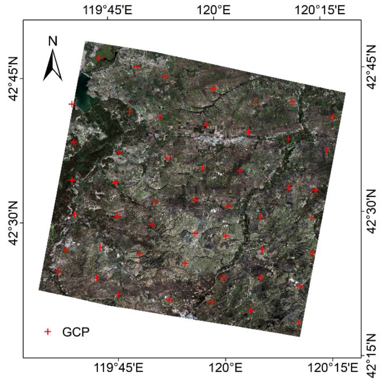
2. Study Area
3. Data
3.1. ZY3-02 Data
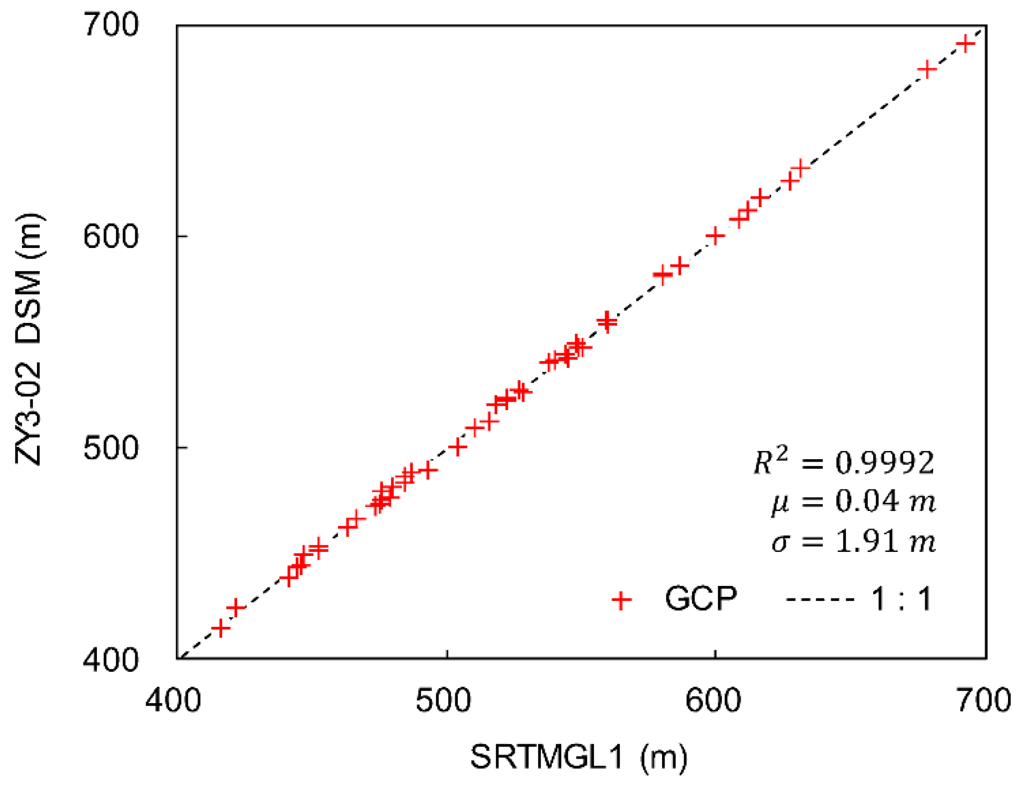
3.2. SRTMGL1 Data
4. Methods
4.1. DSM Extraction
4.2. Sample Selection
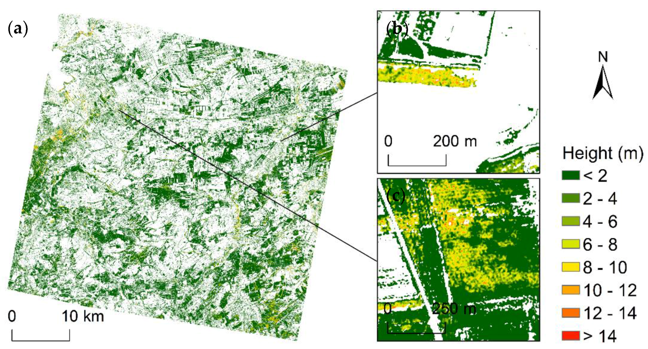
4.3. Canopy Height Modeling and Extrapolation
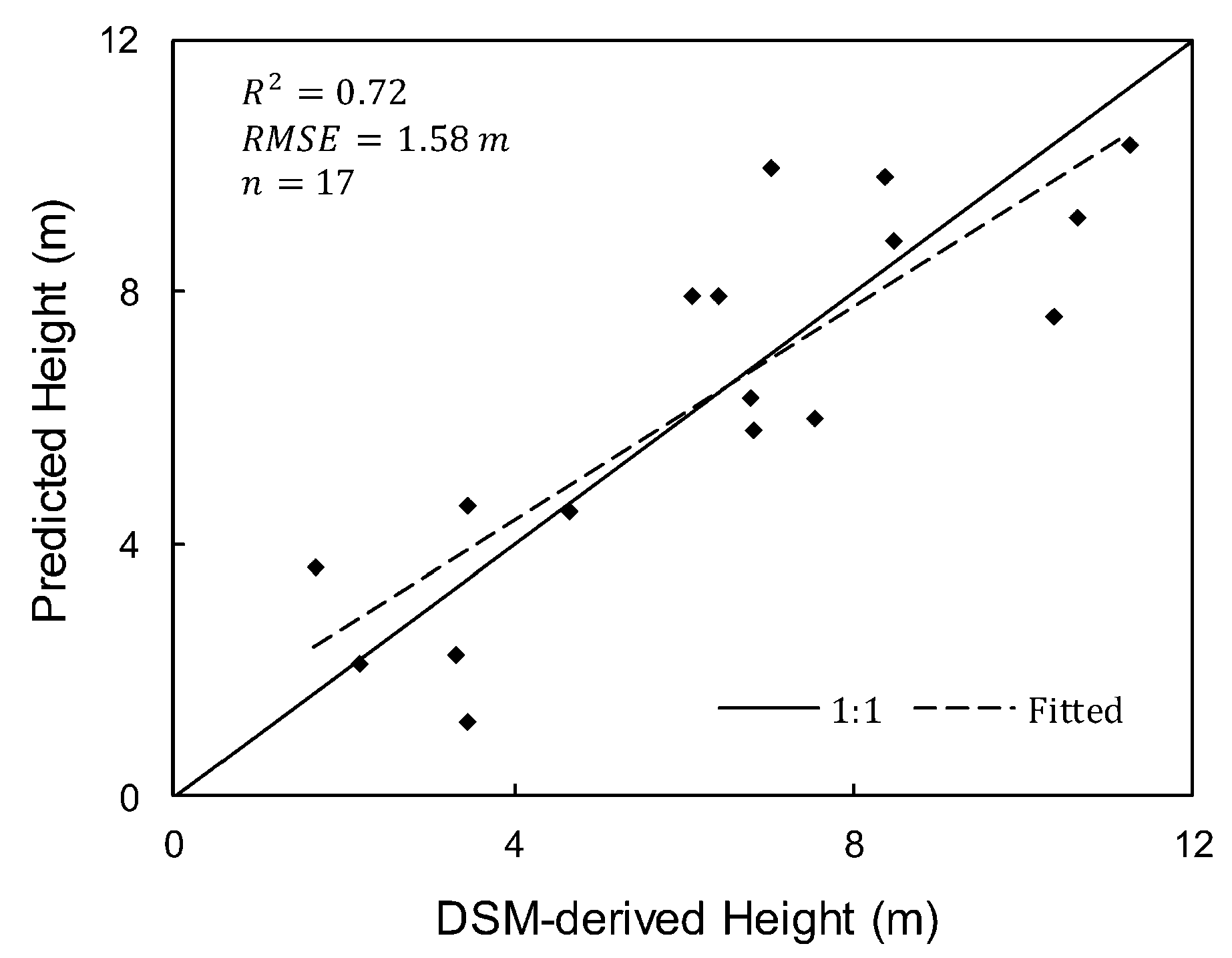
5. Results
6. Discussion
7. Conclusions
Author Contributions
Funding
Acknowledgments
Conflicts of Interest
References
- Drake, J.B.; Dubayah, R.O.; Knox, R.G.; Clark, D.B.; Blair, J.B. Sensitivity of large-footprint lidar to canopy structure and biomass in a neotropical rainforest. Remote Sens. Environ. 2002, 81, 378–392. [Google Scholar] [CrossRef]
- Garcia, O. Dynamical implications of the variability representation in site-index modelling. Eur. J. For. Res. 2011, 130, 671–675. [Google Scholar] [CrossRef]
- Lim, K.; Treitz, P.; Wulder, M.; St-Onge, B.; Flood, M. LiDAR remote sensing of forest structure. Prog. Phys. Geogr. 2003, 27, 88–106. [Google Scholar] [CrossRef]
- Bolton, D.K.; Coops, N.C.; Wulder, M.A. Investigating the agreement between global canopy height maps and airborne LiDAR derived height estimates over Canada. Can. J. Remote Sens. 2013, 39, S139–S151. [Google Scholar] [CrossRef]
- Lefsky, M.A.; Keller, M.; Pang, Y.; De Camargo, P.B.; Hunter, M.O. Revised method for forest canopy height estimation from Geoscience Laser Altimeter System waveforms. J. Appl. Remote Sens. 2007, 1, 1–18. [Google Scholar]
- Lefsky, M.A. A global forest canopy height map from the Moderate Resolution Imaging Spectroradiometer and the Geoscience Laser Altimeter System. Geophys. Res. Lett. 2010, 37, 1–5. [Google Scholar] [CrossRef]
- Simard, M.; Pinto, N.; Fisher, J.B.; Baccini, A. Mapping forest canopy height globally with spaceborne lidar. J. Geophys. Res. Biogeosci. 2011, 116, G04021. [Google Scholar] [CrossRef]
- Huang, H.; Liu, C.; Wang, X.; Biging, G.S.; Chen, Y.; Yang, J.; Gong, P. Mapping vegetation heights in China using slope correction ICESat data, SRTM, MODIS-derived and climate data. ISPRS J. Photogramm. Remote Sens. 2017, 129, 189–199. [Google Scholar] [CrossRef]
- Hansen, M.C.; Potapov, P.V.; Goetz, S.J.; Turubanova, S.; Tyukavina, A.; Krylov, A.; Kommareddy, A.; Egorov, A. Mapping tree height distributions in Sub-Saharan Africa using Landsat 7 and 8 data. Remote Sens. Environ. 2016, 185, 221–232. [Google Scholar] [CrossRef]
- Neuenschwander, A.; Pitts, K. The ATL08 land and vegetation product for the ICESat-2 Mission. Remote Sens. Environ. 2019, 221, 247–259. [Google Scholar] [CrossRef]
- Qi, W.; Dubayah, R.O. Combining Tandem-X InSAR and simulated GEDI lidar observations for forest structure mapping. Remote Sens. Environ. 2016, 187, 253–266. [Google Scholar] [CrossRef]
- Karjalainen, M.; Kankare, V.; Vastaranta, M.; Holopainen, M.; Hyyppä, J. Prediction of plot-level forest variables using TerraSAR-X stereo SAR data. Remote Sens. Environ. 2012, 117, 338–347. [Google Scholar] [CrossRef]
- Capaldo, P.; Nascetti, A.; Porfiri, M.; Pieralice, F.; Fratarcangeli, F.; Crespi, M.; Toutin, T. Evaluation and comparison of different radargrammetric approaches for Digital Surface Models generation from COSMO-SkyMed, TerraSAR-X, RADARSAT-2 imagery: Analysis of Beauport (Canada) test site. ISPRS J. Photogramm. Remote Sens. 2015, 100, 60–70. [Google Scholar] [CrossRef]
- Balzter, H.; Rowland, C.S.; Saich, P. Forest canopy height and carbon estimation at Monks Wood National Nature Reserve, UK, using dual-wavelength SAR interferometry. Remote Sens. Environ. 2007, 108, 224–239. [Google Scholar] [CrossRef]
- Solberg, S.; Astrup, R.; Breidenbach, J.; Nilsen, B.; Weydahl, D. Monitoring spruce volume and biomass with InSAR data from TanDEM-X. Remote Sens. Environ. 2013, 139, 60–67. [Google Scholar] [CrossRef]
- Zhang, Y.; He, C.; Xu, X.; Chen, D. Forest vertical parameter estimation using PolInSAR imagery based on radiometric correction. ISPRS Int. J. Geo-Inf. 2016, 5, 186. [Google Scholar] [CrossRef]
- Ghasemi, N.; Tolpekin, V.; Stein, A. A modified model for estimating tree height from PolInSAR with compensation for temporal decorrelation. Int. J. Appl. Earth Obs. 2018, 73, 313–322. [Google Scholar] [CrossRef]
- Cloude, S.R.; Papathanassiou, K.P. Polarimetric SAR interferometry. IEEE Trans. Geosci. Remote Sensing 1998, 36, 1551–1565. [Google Scholar] [CrossRef]
- Yamada, H.; Yamaguchi, Y.; Rodriguez, E.; Kim, Y.; Boerner, W.M. Polarimetric SAR interferometry for forest canopy analysis by using the super-resolution method. In Proceedings of the 2001 IEEE International Geoscience and Remote Sensing Symposium (IGARSS), Sydney, Australia, 9–13 July 2001; pp. 1101–1103. [Google Scholar]
- Papathanassiou, K.P.; Hajnsek, L.; Moreira, A.; Cloude, S.R. Interferometric SAR polarimetry using a passive polarimetric microsatellite concept. In Proceedings of the 2002 IEEE International Geoscience and Remote Sensing Symposium (IGARSS), Toronto, Canada, 24–28 June 2002; pp. 826–828. [Google Scholar]
- Cloude, S.R.; Papathanassiou, K.P. Three-stage inversion process for polarimetric SAR interferometry. IEE Proc. Radar Sonar Navig. 2003, 150, 125–134. [Google Scholar] [CrossRef]
- Le Toan, T.; Quegan, S.; Davidson, M.W.J.; Balzter, H.; Paillou, P.; Papathanassiou, K.; Plummer, S.; Rocca, F.; Saatchi, S.; Shugart, H.; et al. The BIOMASS mission: Mapping global forest biomass to better understand the terrestrial carbon cycle. Remote Sens. Environ. 2011, 115, 2850–2860. [Google Scholar] [CrossRef]
- Moreira, A.; Krieger, G.; Hajnsek, I.; Papathanassiou, K.; Younis, M.; Lopez-Dekker, P.; Huber, S.; Villano, M.; Pardini, M.; Eineder, M.; et al. Tandem-L: A Highly Innovative Bistatic SAR Mission for Global Observation of Dynamic Processes on the Earth’s Surface. IEEE Geosc. Rem. Sens. M. 2015, 3, 8–23. [Google Scholar] [CrossRef]
- Leberl, F.; Irschara, A.; Pock, T.; Meixner, P.; Gruber, M.; Scholz, S.; Wiechert, A. Point clouds: Lidar versus 3D vision. Photogramm. Eng. Remote Sens. 2010, 76, 1123–1134. [Google Scholar] [CrossRef]
- White, J.C.; Wulder, M.A.; Vastaranta, M.; Coops, N.C.; Pitt, D.; Woods, M. The utility of image-based point clouds for forest inventory: A comparison with airborne laser scanning. Forests 2013, 4, 518–536. [Google Scholar] [CrossRef]
- Aguilar, M.A.; Del Mar Saldaña, M.; Aguilar, F.J. Generation and quality assessment of stereo-extracted DSM from GeoEye-1 and WorldView-2 imagery. IEEE Trans. Geosci. Remote Sens. 2014, 52, 1259–1271. [Google Scholar] [CrossRef]
- Herrero, H.M.; Felipe, G.B.; Belmar, L.S.; Hernandez, L.D.; Rodriguez, G.P.; Gonzalez, A.D. Dense Canopy Height Model from a low-cost photogrammetric platform and LiDAR data. Trees-Struct. Funct. 2016, 30, 1287–1301. [Google Scholar] [CrossRef]
- Immitzer, M.; Stepper, C.; Böck, S.; Straub, C.; Atzberger, C. Use of WorldView-2 stereo imagery and National Forest Inventory data for wall-to-wall mapping of growing stock. For. Ecol. Manage. 2016, 359, 232–246. [Google Scholar] [CrossRef]
- Véga, C.; St-Onge, B. Height growth reconstruction of a boreal forest canopy over a period of 58 years using a combination of photogrammetric and lidar models. Remote Sens. Environ. 2008, 112, 1784–1794. [Google Scholar] [CrossRef]
- Cohen, W.B.; Spies, T.A. Remote sensing of canopy structure in the pacific northwest. Northwest Environ. J. 1990, 6, 415–418. [Google Scholar]
- Cohen, W.B.; Spies, T.A. Estimating structural attributes of Douglas-fir/western hemlock forest stands from Landsat and SPOT imagery. Remote Sens. Environ. 1992, 41, 1–17. [Google Scholar] [CrossRef]
- Hudak, A.T.; Lefsky, M.A.; Cohen, W.B.; Berterretche, M. Integration of lidar and Landsat ETM+ data for estimating and mapping forest canopy height. Remote Sens. Environ. 2002, 82, 397–416. [Google Scholar] [CrossRef]
- Xu, K.; Jiang, Y.; Zhang, G.; Zhang, Q.; Wang, X. Geometric Potential Assessment for ZY3-02 Triple Linear Array Imagery. Remote Sens. 2017, 9, 658. [Google Scholar] [CrossRef]
- Farr, T.G.; Rosen, P.A.; Caro, E.; Crippen, R.; Duren, R.; Hensley, S.; Kobrick, M.; Paller, M.; Rodriguez, E.; Roth, L.; et al. The Shuttle Radar Topography Mission. Rev. Geophys. 2007, 45, 1–43. [Google Scholar] [CrossRef]
- Hu, Z.; Peng, J.; Hou, Y.; Shan, J. Evaluation of recently released open global digital elevation models of Hubei, China. Remote Sens. 2017, 9, 262. [Google Scholar] [CrossRef]
- Hirschmuller, H. Stereo Processing by Semiglobal Matching and Mutual Information. IEEE Trans. Pattern Anal. Mach. Intell. 2008, 30, 328–341. [Google Scholar] [CrossRef] [PubMed]
- Richter, R.; Schläpfer, D.; Müller, A. An automatic atmospheric correction algorithm for visible/NIR imagery. Int. J. Remote Sens. 2006, 27, 2077–2085. [Google Scholar] [CrossRef]
- Williams, M.S.; Bechtold, W.A.; Labau, V.J. Five instruments for measuring tree heights: An evaluation. South. J. Appl. For. 1994, 18, 76–82. [Google Scholar]


| Area (m2) | DSM Pixels | Mean Elevation (m) | |
|---|---|---|---|
| Canopy samples | 748–22,864 | 187–5,716 | 420–614 |
| Ground samples | 620–17,288 | 155–4,322 | 415–611 |
© 2019 by the authors. Licensee MDPI, Basel, Switzerland. This article is an open access article distributed under the terms and conditions of the Creative Commons Attribution (CC BY) license (http://creativecommons.org/licenses/by/4.0/).
Share and Cite
Liu, M.; Cao, C.; Chen, W.; Wang, X. Mapping Canopy Heights of Poplar Plantations in Plain Areas Using ZY3-02 Stereo and Multispectral Data. ISPRS Int. J. Geo-Inf. 2019, 8, 106. https://doi.org/10.3390/ijgi8030106
Liu M, Cao C, Chen W, Wang X. Mapping Canopy Heights of Poplar Plantations in Plain Areas Using ZY3-02 Stereo and Multispectral Data. ISPRS International Journal of Geo-Information. 2019; 8(3):106. https://doi.org/10.3390/ijgi8030106
Chicago/Turabian StyleLiu, Mingbo, Chunxiang Cao, Wei Chen, and Xuejun Wang. 2019. "Mapping Canopy Heights of Poplar Plantations in Plain Areas Using ZY3-02 Stereo and Multispectral Data" ISPRS International Journal of Geo-Information 8, no. 3: 106. https://doi.org/10.3390/ijgi8030106
APA StyleLiu, M., Cao, C., Chen, W., & Wang, X. (2019). Mapping Canopy Heights of Poplar Plantations in Plain Areas Using ZY3-02 Stereo and Multispectral Data. ISPRS International Journal of Geo-Information, 8(3), 106. https://doi.org/10.3390/ijgi8030106