How They Move Reveals What Is Happening: Understanding the Dynamics of Big Events from Human Mobility Pattern

1. Introduction

The analysis of mobility data, obtained from tracking moving objects, has attracted a high research interest. However, as pointed out by recent studies in this domain [1,2] the progress in analysing mobility data has generally left out the movement context, which is rather an important factor for understanding the movement. The movement context is the set of elements that can characterise the situation in which the movement takes place. Context elements include, among others, static objects, the geographic space where the movement takes place, and events occurring in this space. A context element may be static or dynamic. For a static context element, the values of its attributes considered by a study remain unchanged during the period of the study. For example, in a place recommender system where the objective is to provide tourists with locations of attractive places and respective types of attractions, the location and activity of a place remain unchanged and hence the place is a static context element. On the other hand, for a dynamic context element, the values of some attributes under consideration by the study change during the period of study. For example, in a transportation planning application with the objective of adapting the transportation capacity to the demand, public social events are dynamic context elements. This is due to the fact that attributes of interest to the application such as the event location and associated mass movement change (the event is geographically located at some time period and then it disappears—shortly before its start there is a large mass movement compared to some time after the start …).

Several studies on mobility data have considered static context elements such as static objects existing in the geographic space [3,4] and other properties of the geographic space [5]. However, dynamic context elements have been rarely considered despite being very common in real life applications of mobility data analysis. Our paper contributes to fill this gap.

Since the movement context is very broad, this paper proposes a methodology for integrating a specific category of movement context elements into the analysis of mobility data. These are characterized by a geographic location and the time period at which they exist. We refer to it as geographic context. We use the term geographic context to set the scope of our study regarding the context of the movement. The context of the movement itself is very broad. It can also include elements internal to the moving object that may affect its movement, which are beyond the scope of our study. However, like the geographic context considered in our study, the context internal to the moving object is also static (e.g., gender) or dynamic (e.g., the hunger level). In particular, we are interested in considering big events as the movement context. This means that we focus on events that attract a large number of people and are of interest to the general public. Furthermore, an event considered in this paper is an event that takes place at a specific known location, such as a football match in a specific stadium or a big concert in a specific theatre.

As shown by previous studies, big events have a major impact on the behaviour of the community, including its mobility pattern [6,7]. Under this consideration, we propose a methodology for analysing human mobility to support an improved understanding of the dynamics of big events. The methodology is designed to answer the following questions: Given the data about the mobility in the neighbourhood of a location known to host big events, (1) did a big event occur? If it occurred, (2) to what extent can we estimate its start and end times? (3) What is the temporal pattern of arrival and departure of event attendees: (a) did they arrive progressively or immediately before the start of the event; (b) did they depart immediately after the end of the event or did they depart progressively, possibly taking some additional time to enjoy the location and/or experience before leaving the site?

The rest of the paper is organised as follows. Section 2 discusses related work while the proposed methodology is explained in Section 3. Section 4 presents an experimental evaluation of the methodology based on real data, and the results of this evaluation are discussed in Section 5. Finally, Section 6 concludes and suggests directions for future work.

2. Related Work

The work presented in this paper is related to a considerable number of studies on the analysis of mobility data. These studies include methods for extracting important places from mobility data. In particular, we apply clustering as a data mining method for detecting stopping locations and associate stopping with corresponding semantic information such as done in [8]. We adopt the concepts of stop and move for segmenting trajectories into episodes as discussed in [9,10] and extract mobility patterns on which we carry out a detailed analysis. Human mobility has been studied using different forms of traces including traces of individuals extracted from their mobile phone data [11] or social network platforms [12], trajectories of private cars [13], and trajectories of taxis [14]. Due to privacy concerns, these data are hardly accessible because they represent traces of individuals. Another problem specific to mobile phone data and social media data is that they have a very low temporal resolution. This problem makes it a big challenge to find mobility patterns from mobile phone and social media data using data mining algorithms.

Studies particularly related to this paper are on integrating the movement context into the analysis of mobility data and the analysis of people’s behaviour in case of events. Andrienko, Andrienko, and Heurich [15] proposed a conceptual model for context-aware analysis of movement. They identified different context element types (e.g., events, time, and space) and provided examples of analysing the relations between the moving object and some of the identified context element types. Buchin et al. [16] also presented different types of context (e.g., obstacles, network, and terrain), which they modelled as a labelled polygon subdivision and took into account while studying the similarity of trajectories. Apart from the above two studies that model the geographic context in general, other context-aware analyses of mobility data consider a single context element type. Commonly considered context elements are geographic points of interest (e.g., [8,17]) and environmental factors, often available as remote sensing imagery such as temperature and altitude (e.g., [5,18]). Despite the important contribution of the above studies on modelling the movement context and exemplifying the integration of some context element types, there is still a need to consider a dynamic context where the time dimension is explicitly studied. In our paper, in addition to static objects we consider events, which exist for a certain time period and go through a number of characteristic phases during the period of existence.

Bagrow, Wang, and Barabási [6] analysed call records from a mobile phone service provider to explore the societal response to different types of events. They analysed two types of events: events categorized as emergencies (e.g., plane crash and quake) and non-emergencies (e.g., concert). Calabrese [7] analysed cell-phone traces to identify the origins of people attending specific events. The events analysed in [7] and the non-emergency events studied in [6] are similar to the events considered in our study. However, these studies are person-based in the sense that the event is known and the focus is on individuals while ours is event-based trying to detect an event at a specific location. Furthermore, the available studies are based on either tracks of individuals (e.g., [19]), requiring a high cooperation, or mobile phone call records, which are not easily accessible and have low spatial and temporal accuracy [11]. Dissimilarly, we use tracks of public transportation vehicles, which have a high spatial and temporal accuracy and do not require the cooperation of travellers.

3. Proposed Methodology

The methodology we propose for integrating movement context into mobility data analysis is based on the “movement as interaction” metaphor [20]. In this metaphor, the movement pattern observed is considered to be a result of the interaction between the moving object and the elements of the context. Interactions represent changes of spatial relations over time (e.g., passing by, approaching, stopping, etc.). The interaction concept in this paper has also been called spatio-temporal relation [15] and pattern [21]. In particular, this paper analyses the interactions between moving objects following a pre-defined route and events occurring in the vicinity of the route.

3.1. Basic Concepts and Definitions

The movement data analysed in this paper represent the movement of an object that moves back and forth between the end points of a pre-defined route. This is the case of scheduled public transportation vehicles such as buses and trams of a known line. The basic assumption on this kind of movement in our study is that the vehicle does not necessarily stop at every designated stop point along the route. For example, when a bus reaches a designated stop point along the route it generally stops if there are passengers waiting to get out or in. In this case though stopping does not determine the exact number of people entering the bus; some attributes associated with the stop provide an indication of the numbers of people moving in the respective direction. For example, a long stop is an indicator that a lot of people are getting in and/or exiting the bus. Likewise, having a large number of stops is an indicator that there are a lot of people getting in and/or exiting the bus. These two cases positively correlate with the number of people taking the bus in that direction. However, whether these passengers are attending the event can be confirmed by also checking the number of stops at the event venue. In this section we introduce the basic concepts related to such movement, which are used in the proposed methodology.

Definition 1.

Journey. A journey is a time-ordered sequence of GPS points recorded along the movement from one end point of the pre-defined route to the other end point.

Definition 2.

Geographic context (or simply context). The geographic context of a movement is a set of elements that characterise the environment where the movement takes place. Context elements can be of different types including the geographic space (e.g., highway and secondary road), static objects (e.g., bus stops, traffic lights), moving objects (e.g., other moving cars and pedestrians), and events (e.g., a football match in a stadium in the vicinity of the route used by the moving object).

Definition 3.

Interaction. We use the term interaction to refer to a process in which a spatial relation between the moving object and a movement context element changes over time. Several types of interactions can be defined depending on the type of context element, but in this paper we are interested in three interactions only (stopping, approaching, and moving-away), which are illustrated in Figure 1 and defined next.

Definition 4.

Stopping. A stopping interaction happens when the initially moving object stays in the neighbourhood of the context element for a certain time threshold. Let A be a moving object, C be a context element modelled as a point, and t be a time instant at which the position of the moving object was recorded. Let d(A, C, t) denote the distance between A and C at the time instant t, nParam be a neighbourhood parameter, and S_min be the minimum amount of time a stopping should last. The Stopping interaction is formalised as follows:

$$\begin{gathered} \exists t_i, t_j, t_k | t_i<t_j<t_k \\ \forall t,t_j\le t<t_k: d\left(A,C,t\right)\le nParam \wedge t_k-t_j\ge S_{min} \wedge d\left(A,C,t_i\right)>nParam \end{gathered}$$

Definition 5.

Approaching. The approaching interaction is observed when the distance between the moving object and the context element decreases. This is formalised as follows:

$$\begin{gathered} \exists t_g, t_h | t_h>t_g \\ d\left(A,C,t_h\right)-d\left(A,C,t_g\right)<0 \end{gathered}$$

Definition 6.

Moving-away. The moving-away interaction is observed when the distance between the moving object and the context element increases. This is formalised as follows:

$$\begin{gathered} \exists t_l, t_m | t_m>t_l \\ d\left(A,C,t_m\right)-d\left(A,C,t_l\right)>0 \end{gathered}$$

3.2. Methods

This paper focuses on two context elements: known stop points along the route, and a potential event at a known location. The former category forms a static context while the latter forms a dynamic context according to the definition of movement context given in Section 1. The approach we propose involves two main steps: extracting interactions from the mobility data, and performing a spatio-temporal analysis of the extracted interactions.

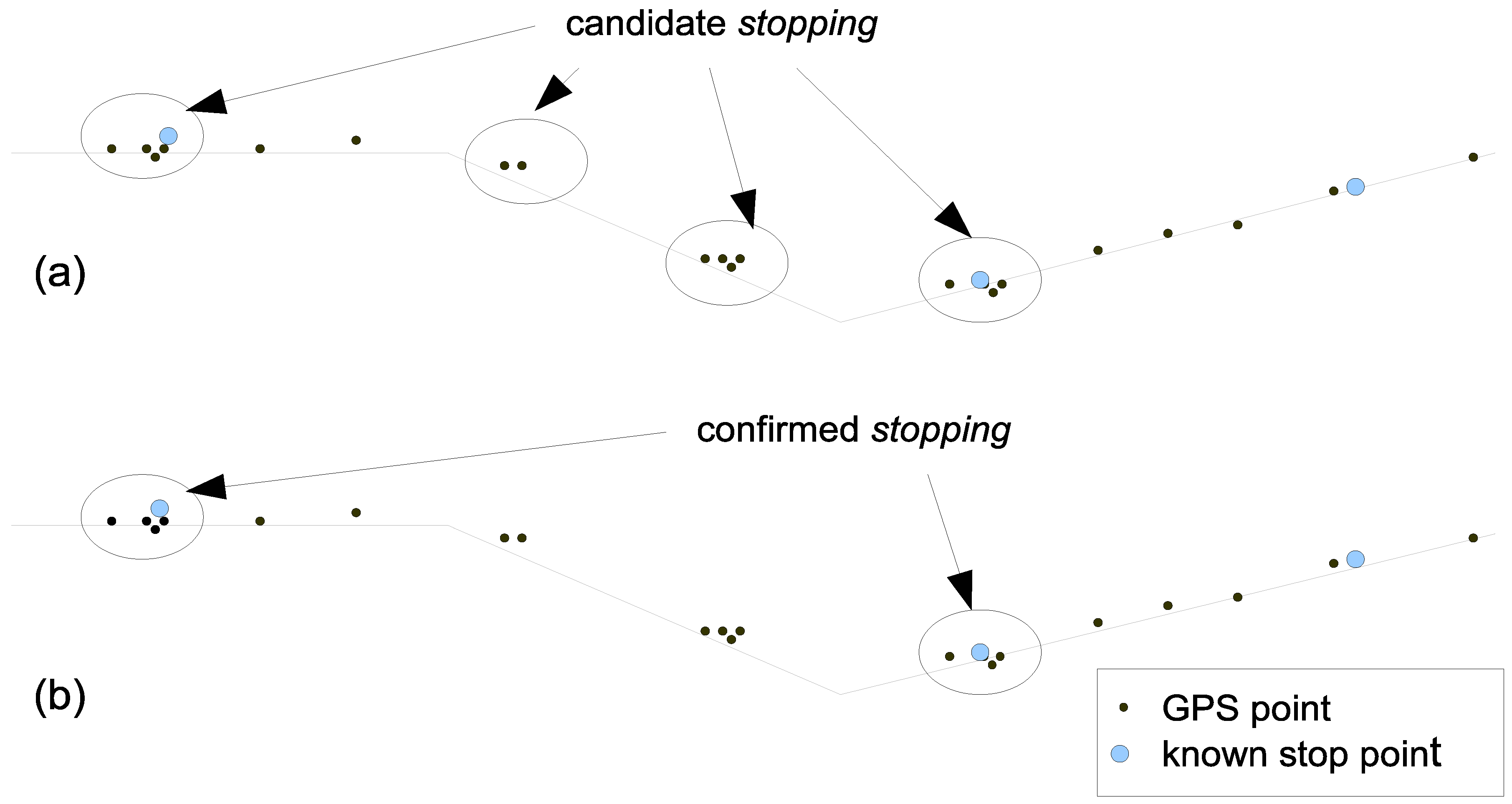
3.2.1. Extracting Interactions

The mobility data generally contain noise and errors that need to be cleaned in a pre-processing step. The cleaning needed depends on the quality of the available data. As a minimum requirement, the type of data processed in this paper needs to be pre-processed to identify individual journeys. After the pre-processing step, each journey is analysed to detect the occurrence of stopping, approaching, and moving-away interactions.

(1) Stopping interaction

The extraction of stopping interactions considers the locations of stop points (e.g., bus or tram stops) along the route as context elements. The objective is to extract actual occurrences of stopping at these context elements. The consideration behind the process is the fact that the initially moving object stays in the neighbourhood of the context element for at least a specified amount of time. We implement the extraction of stoppings in two steps following the approach in [22]. In the first step, considering that a normal position recording will produce more closely located points during a stopping, we adopt a form of density-based clustering to extract candidate stoppings (See Figure 2a). The parameters for this clustering are set based on the characteristics of the data. In the second step, we check and discard all candidate stoppings obtained from the first step which do not lie within the neighbourhood of a known stop point (See Figure 2b).

(2) Approaching and moving-away interactions

The aim is, for each journey, to identify the section where the moving object is approaching the event and the section where it is moving away from the event. From each route end we identify the known stop point closest to the event location taking into account the road segment providing access to the event location from the route. These two stop points form reference points in the two directions of the route for identifying journey sections. Based on the journey direction and the variation of the distance along the route to the respective reference point we mark the journey points. When the distance decreases, the point is marked to be on an approaching section and when it increases, it is marked to be on a moving-away section. When the distance does not change the marking is deferred until next change. This process follows the definitions of approaching and moving-away given earlier.

After the extraction of interactions each journey position is marked according to whether it is part of a stopping interaction or not, and on the approaching or moving-away section of the journey. From the computed interactions the next step extracts features that are then used for a spatio-temporal analysis.

3.2.2. Spatio-Temporal Analysis of Interactions

This step starts by extracting mobility characteristic features. For each journey, we count the stoppings made while approaching the event (approaching stoppings) and those made while going away from the event (moving-away stoppings). Since the number of stop points on the approaching section may be different from that on the moving-away section, we normalise the two variables (number of approaching stoppings (Sa) and number of moving-away stoppings (Sg)), hence obtaining the proportion of approaching stoppings (Sa’) and the proportion of moving-away stoppings (Sg’):

$$S{a}^{\text{'}}=\frac{Sa}{n} and S{g}^{\text{'}}=\frac{Sg}{m}$$

(1)

where n is the number of stop points on the approaching section and m is the number of stop points on the moving-away section.

We discretise each day of movement into 1-h intervals. Then we derive the stoppings balance (V) from the above two variables, with the stoppings balance being the average of the differences between the proportion of approaching stoppings and the proportion of moving-away stoppings, both of which can be computed for each time interval. For a given time interval i the value of V is computed as follows:

$$V_i=\frac{1}{n}{\displaystyle \sum }_{j=1}^n(S{a_j}^{\text{'}}-S{g_j}^{\text{'}})$$

(2)

where n is the number of journeys that passed at the event venue during the time interval i.

We then define the normal stoppings balance (W) as the average of the stoppings balances during “normal conditions”. In other words, for a given time interval the normal stoppings balance W is the average of the stoppings balances of the time intervals of same hour of the day and same day of the week but only in periods confirmed to be without event at the considered event venue. For a given time interval i the value of W is computed as follows:

$$W_i=\frac{1}{k}{{\displaystyle \sum }}_{j=1}^k{V}_j$$

(3)

where k is the number of time intervals having the same hour of the day and same day of the week as i, but which have been confirmed to be event free at the event venue.

From the definition of W it follows that this variable has one value for each 1-h interval of each day of the week and the greater the number of days without the event occurring during this time interval that are considered the more accurate this value is.

We also compute the number of stoppings near the venue (P) as the number of stoppings in a neighbourhood of the event venue which allows for the consideration of all stop points that directly serve the venue irrespective of the line. For example, we used a radius of 650 m (see Figure 3a) around the stadium to capture stoppings at all bus stops that serve the stadium directly from different bus lines. In the same way we derived the normal stoppings balance from the stoppings balance, we compute the normal number of stoppings near the venue (Q) as the average of the number of stoppings near the venue during periods without event at the event venue.

The detection of an event is based on the analysis of the variation of the above four variables (V, W, P, Q). The reasoning behind using these variables is that in case of an event we expect to see two time intervals with a high increase of the value of P above the value of Q. The two intervals correspond to the arrival and departure of event attendees. The specific interval corresponding to arrival and the one corresponding to departure can be identified from the variation of V with respect to W. In order to analyse the variation of these variables we compute the upper and lower bounds. The upper bound (UV) and lower bound (LV) of V are computed as follows:

$$\begin{gathered} U{V}_i=W_i+a{\sigma }_w \\ L{V}_i=W_i-a{\sigma }_w \end{gathered}$$

(4)

where α is a scale factor and ${\sigma }_{\mathrm{w}}$ is the standard deviation of V in normal conditions.

Similarly, we compute the upper bound (UP) of P as follows:

$$U{P}_i=Q_i+a{\sigma }_Q$$

(5)

where α is a scale factor and ${\sigma }_Q$ is the standard deviation of P in normal conditions.

A high value of V above W means more approaching stoppings than moving-away stoppings, which may mean the movement of a lot of people to the event venue and hence the arrival of event attendees. Following the same reasoning, a low value of V below W may mean the movement of a lot of people away from the event venue, which may indicate individuals departing from the event venue. The comparison of P with its related variables (Q and UP) produces candidate times for arrival and departure, which are confirmed or rejected using the comparison of V to its related variables (W, UV, and LV). The confirmation of candidate arrival and departure times eventually leads to the detection of event occurrence and an estimation of its start and end time.

In order to explore the arrival to and departure from the event, we perform a local analysis at a finer temporal granularity level. To this end, we analyse the number of stoppings near the venue during smaller time intervals around the departure and arrival times confirmed in the preceding step.

4. Experimental Evaluation

In this section we apply the proposed methodology to real data to evaluate its applicability. We selected the following two cases studies: one involving a stadium as the venue for big events and the other involving a concert hall as a venue for medium to large scale events. We use the first case to explain in detail how the methodology is applied while for the second case we present some results and discuss them. First, we describe the data used and then the analysis of these data using the proposed methodology.

4.1. Data Description and Pre-Processing

4.1.1. Data Description

The data we use in our experiments include mobility data and locations of context elements. The mobility data are trajectories of buses that run on lines 4 and 44 of the Dublin Bus. This is a subset of the Dublin bus GPS dataset [23] from the Dublin City Council’s traffic control. Each bus produces a record regarding its location and status every 20 s on average. The record includes a timestamp, latitude and longitude of the location, the bus line ID, the vehicle ID, the journey pattern (an indication of the direction), an identifier of the closest bus stop, the delay (number of seconds for which the bus is behind schedule, which is negative if the bus is ahead of schedule), whether the bus is at a bus stop, and whether the bus is in a congestion.

The data about context elements include the locations of bus stops along the routes used by the two bus lines, and the locations of the Aviva stadium and the National Concert Hall where events take place. These context elements are depicted in Figure 3. The left part of the figure (a) shows the route used by bus line 4. This route has a length of approximately 20 km and includes 65 bus stops in one direction and 61 stops in the other direction. The right part of the figure (b) shows the route used by bus line 44, which includes 80 bus stops in one direction and 76 stops in the other direction. Also shown in Figure 3 are the neighbourhoods of the event venues defined by a radius of 650 m around the stadium and 350 m around the concert hall. The sizes of these neighbourhoods are selected to enclose all bus stops that directly serve the venues such that a passenger dropped there may not take any other bus to reach the venue. For each bus stop the data include a unique identifier, a name, GPS coordinates, and the distance at which it is located from the beginning of the route.

We retrieved from the Internet information about big events that took place in the Aviva stadium during the time period covered by the mobility data. This information (see

Table 1. Occurrences of big events in the stadium during the study period.

Date	Event	Planned Stiles Opening Time	Planned Start Time	Planned End Time	Actual End Time	Number of Attendees
10 November 2012	Rugby match (Ireland vs. South Africa)	16:00	17:30	19:00	19:20	49,781
14 November 2012	Football match (Ireland vs. Greece)	18:15	19:45	21:45	21:42	16,256
24 November 2012	Rugby match (Ireland vs. Argentina)	12:30	14:00	15:40	15:49	43,406

) has been retrieved from the Website of the National Police Service of Ireland [24] and the Wikipedia website. Likewise, we retrieved from the Internet information about the concerts that took place in the National Concert hall in the period covered by the mobility data. Events were regularly organized around 8:30 pm as seen from the event archive website [25].

4.1.2. Data Pre-Processing

In order to prepare the data for analysis we performed the following pre-processing operations. We performed time format and coordinate system transformations. Next, we cleaned the data by removing unrealistic positions. For example, if the segment between a position and its direct predecessor appeared to have been travelled at an average speed higher than 50 km/h, we considered this position unrealistic and discarded it. Although each recorded bus position was associated with an identifier of the closest bus stop, we found wrongly assigned identifiers, where the identifiers were different from the unique identifiers of bus stops. Therefore, we recomputed the closest bus stop for each recorded bus position. Sometimes we saw, from the sequence of positions, oscillation backwards and forwards along the route. Since each successive GPS record must progress along the route we identified the GPS records that caused such oscillation and removed them. Such records were identified by comparing the distances at which the closest bus stop and that of its direct predecessor were located. The cleaned bus positions match well with the road network.

Since the processing and analysis of the bus trajectories is centred on journeys, we proceeded to find individual journeys and assign them unique identifiers. We also labelled each journey with its direction because the journey direction is important in the analysis step. The next step was to clean journeys by removing incomplete journeys. We removed journeys which contain a large gap in space or in time between any two consecutive recorded positions. We consider that a journey must begin and end within a reasonable distance from the first and last bus stops, respectively, along its route. By checking the closest bus stop for the first and last positions in each journey we identified and removed journeys that were incomplete at their start or end. We have considered journeys made between 6:00 and 23:00 because an exploration of the data showed us that this is the period containing a sufficient number of journeys for every day studied. The final clean bus data contains 2249 journeys made on 28 days between November 2012 and January 2013. This period includes three days (10, 14, and 24 November 2012) with big events in the Aviva stadium.

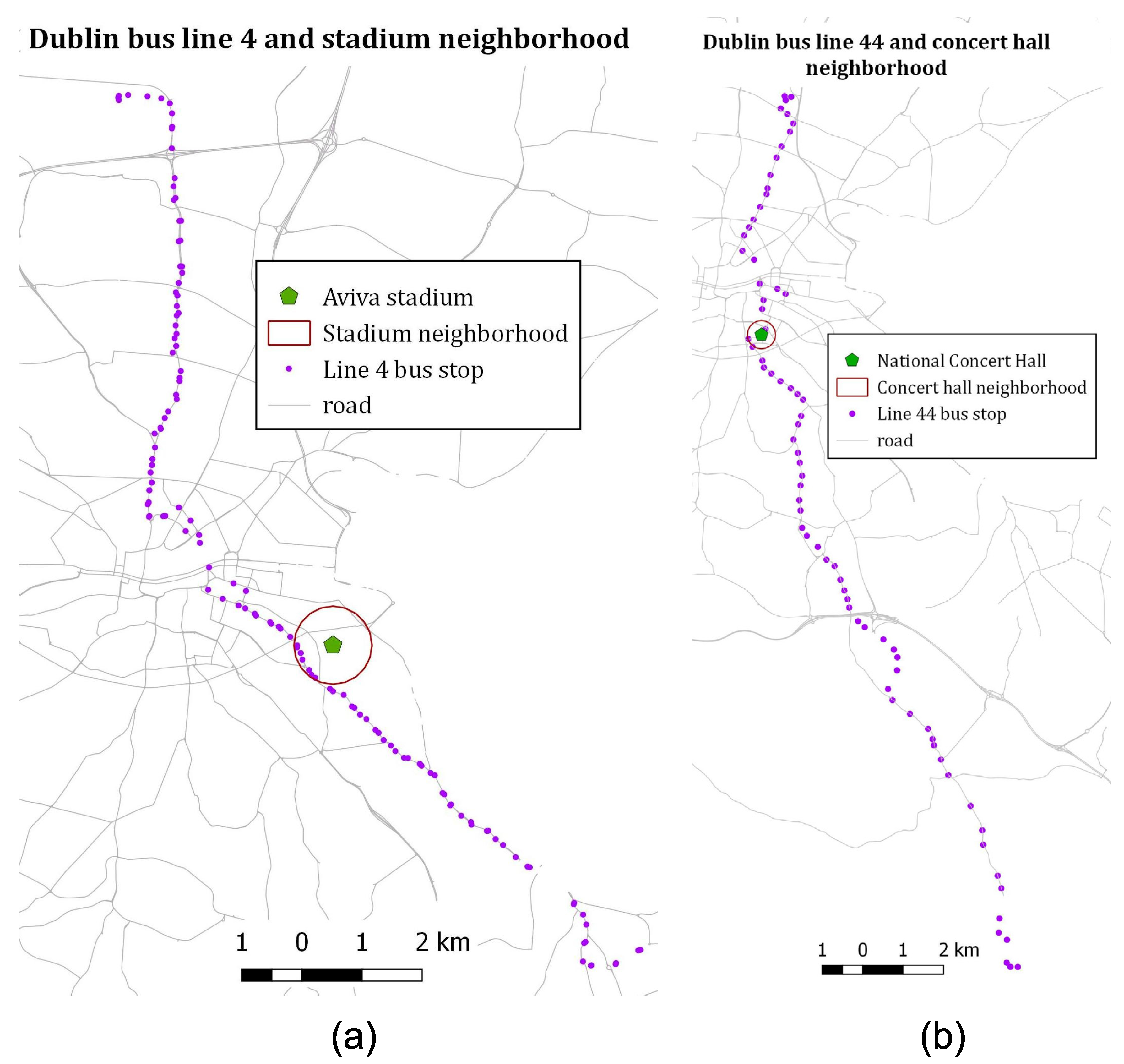
4.2. Extracting Interactions from Mobility Data and the Context of Large-Scale Events in the Aviva Stadium

For extracting stopping interactions, we followed the procedure explained in Section 3.2.1. After experimenting with different parameter value combinations for detecting an obvious stopping (e.g., a stopping in which several points are recorded at the end of a journey) we selected 20 m as the neighbourhood distance and a minimum of two points for density-based clustering. Considering the GPS accuracy of 20 m, we understood that a normal GPS position recording at a bus stop can fall outside of up to 20 m of the bus stop without being an outlier that needs to be discarded. Therefore, we selected 20 m as a neighbourhood parameter on bus stops (nParam). In order to ensure that we detect even a short stopping we had selected the minimum of two points for clustering considering that the GPS sampling rate of 20 s will not produce many points at a bus stop. Furthermore, with the same aim to avoid missing short stopping and based on common sense we selected a minimum stopping duration (S_min) of 10 s.

For extracting approaching and moving-away interactions, we used the distance along the route from the reference bus stops as explained in Section 3.2.1. If the distance from the reference point to the current point is smaller than the distance to the immediate preceding point the current point is on the approaching section, otherwise it is on the moving-away section. An example of the result of interaction extraction is shown in Figure 4. On the journey segment shown each position has been identified either as not part of a stopping, or as part of an approaching stopping, or as part of a moving-away stopping.

4.3. Spatio-Temporal Analysis of Interactions for the Context of Large Scale Events on Aviva Stadium

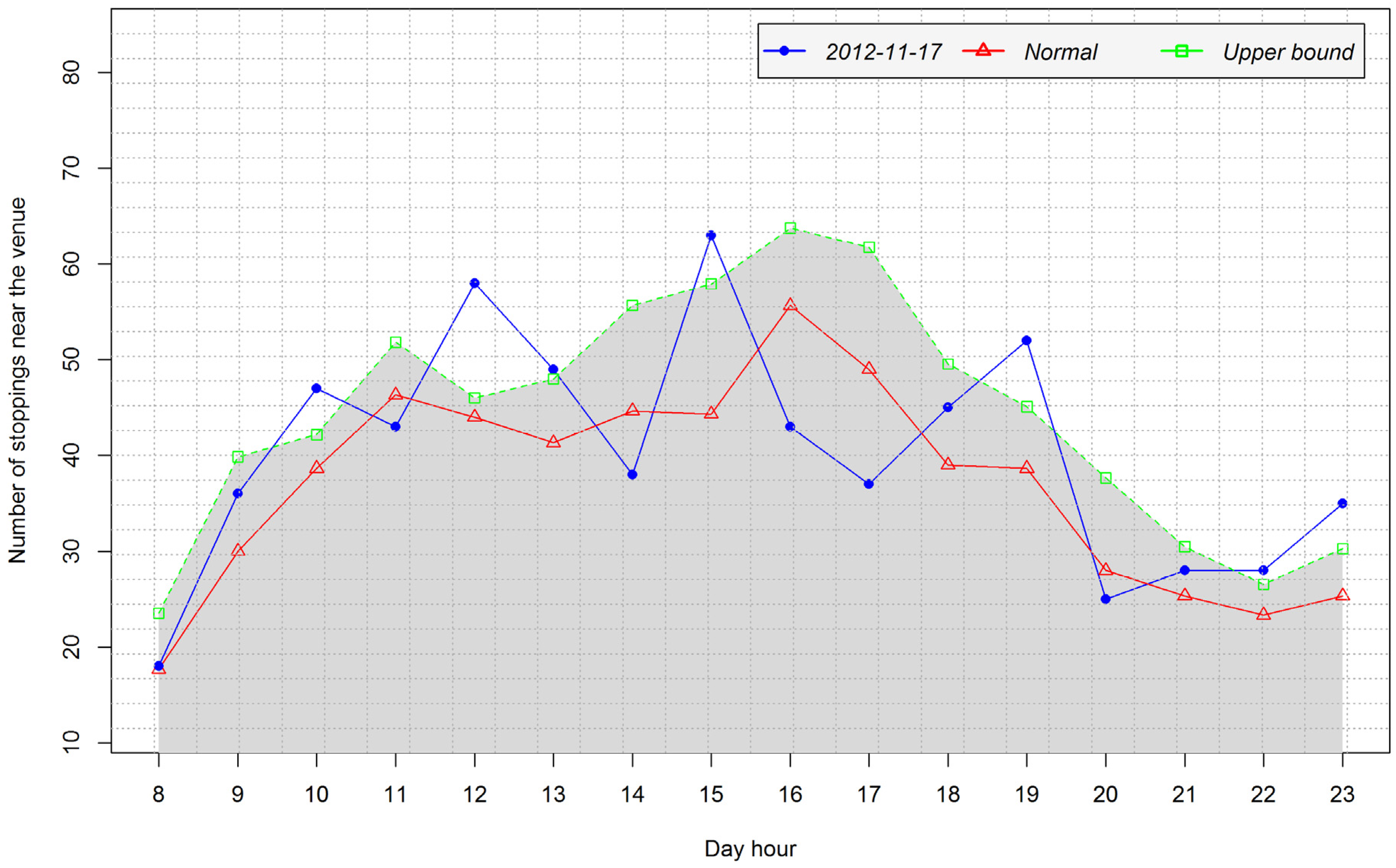
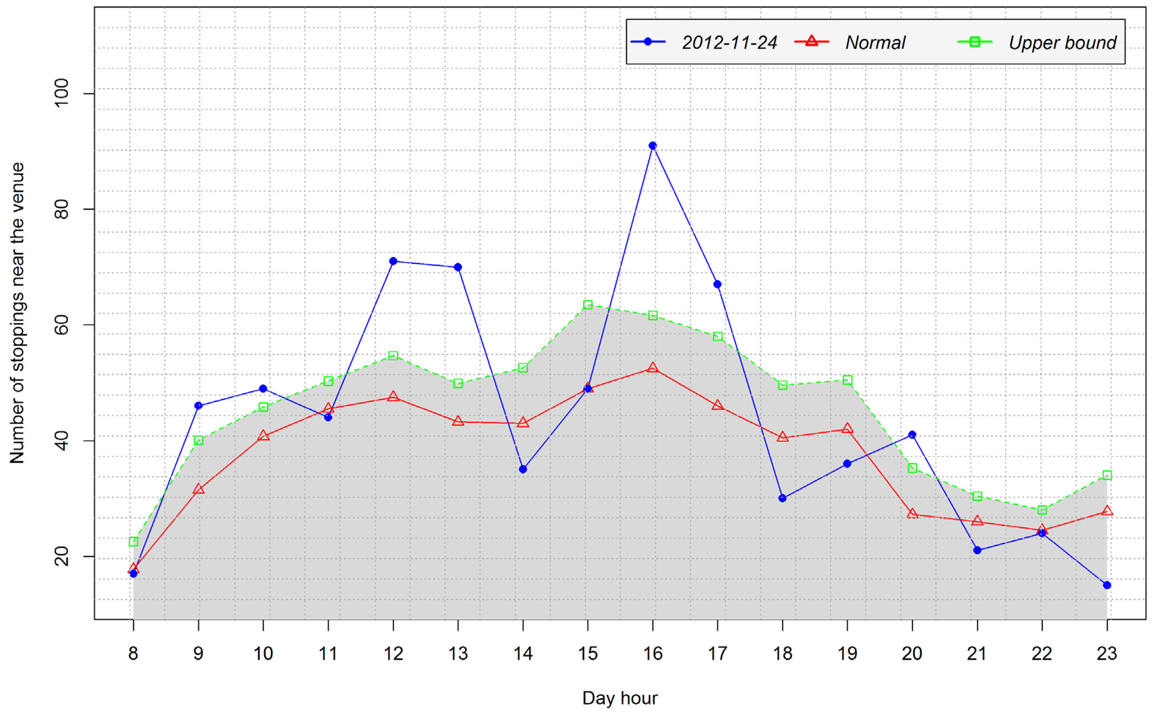
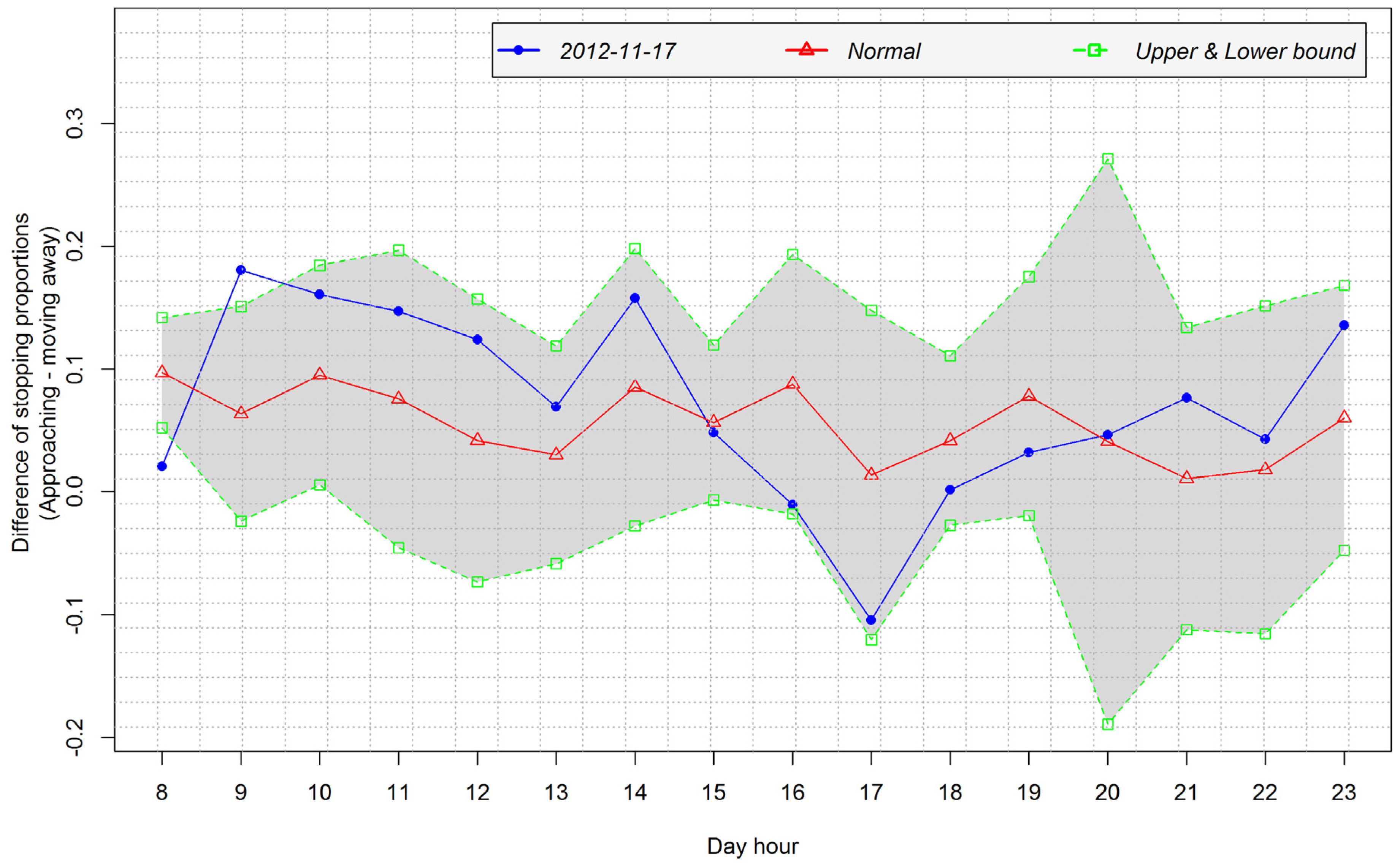
4.3.1. Detection of Arrival and Departure Times

For the discovery of an event and estimation of its start and end time we analyse the general pattern during the period between 6:00 and 23:00 on different days. To this end, we split the period into 1-h intervals and then compute the stoppings balance (V), the normal stoppings balance (W), the number of stoppings near the venue (P), and the normal number of stoppings near the venue (Q) for each interval following the procedure explained in Section 3.2.2. From these values, we derived the values of upper and lower bounds following the procedure explained in Section 3.2.2. We use the value 1 as scale factor (α). Since we need to use both the highest and lowest values of the variable V we compute both its upper bound (UV) and lower bound (LV). On the other hand, we compute only the upper bound for P because we need to use only the highest values. Figure 5 shows the variation of P and its related variables Q, and UP on a sample day without an event while Figure 6 shows the variation of V and its related variables W, UV, and LV on the same day.

In the next step, we analyse the temporal variation of these variables. From the variation of P with respect to its related variables we get candidate event indicators that need to be confirmed using the variation of V with respect to its related variables. That is, the peaks of P that exceed the corresponding upper bound values are candidate event delimiters in time (arrival and departure). It is important to note that the peak of P is considered relative to the upper bound; it corresponds to the highest shift above the upper bound (see for example in Figure 8; the peak is at 9:00 and not at 10:00). From the example shown in Figure 5, we have four candidate event delimiters: 10:00, 12:00, 15:00, and 19:00. For each candidate, we take the interval from the last day hour (before it) at which P was below the upper bound to the first day hour (after the candidate) at which P was below the upper bound. This interval allows us to take into account uncertainties due to aggregating data into 1-h intervals; hence we call it the “uncertainty interval”.

We search for a peak in the variation of V (see Figure 6) within the uncertainty interval. We distinguish two types of peaks. If the value at a certain time in the interval is higher than all preceding and following values in the interval, we have a “positive peak”. If the value at a certain time in the interval is less than all preceding and following values in the interval we have “a negative peak”. The time corresponding to a positive peak is a candidate arrival time because it corresponds to an exceptionally high number of approaching stoppings. On the other hand, the time corresponding to a “negative peak” is a candidate departure time, because it corresponds to an exceptionally high number of moving-away stoppings.

While searching for peaks within an uncertainty interval, the peak found is labelled with its peak level and type. These values are used to determine the type of candidate (arrival time, departure time) and to confirm or reject the candidate. The search for a peak within an uncertainty interval has one of the following seven possible results:

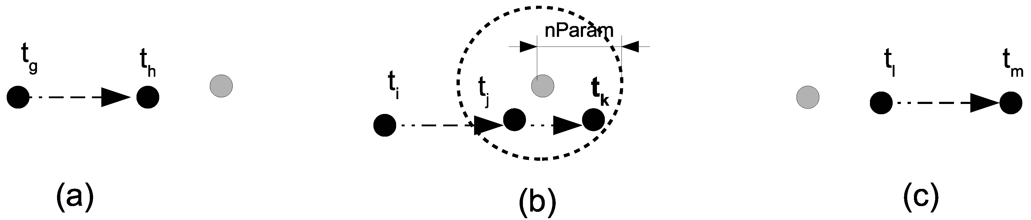
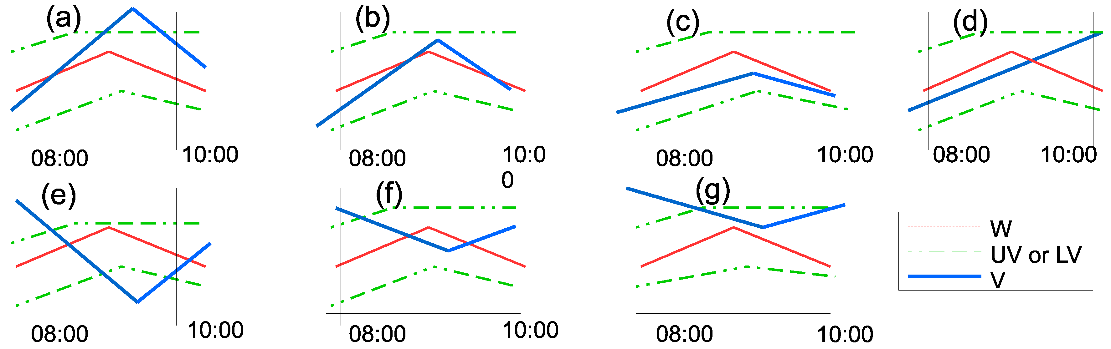
• No peak is found (see Figure 7d). The peak type is set to 0.
• A “positive peak” is found. The peak type is set to 1.

  (a)

  The value b at the peak is such that b > UV_i (see Figure 7a). The peak level is set to 1.

  (b)

  The value b at the peak is such that W_i < b ≤ UV_i (see Figure 7b). The peak level is proportionally calculated based on the relation between UV and W (see Equation 4).

  (c)

  The value b at the peak is such that b ≤ W_i (see Figure 7c). The peak level is set to 0.

• A “negative peak” is found. The peak type is set to −1.

  (a)

  The value b at the peak is such that b < LV_i (see Figure 7e). The peak level is set to 1.

  (b)

  The value b at the peak is such that LV_i ≤ b < W (see Figure 7f). The peak level is proportionally calculated based on the relation between LV and W (see Equation (4)).

  (c)

  The value b at the peak is such that W_i ≤ b (see Figure 7g). The peak level is set to 0.

Any candidate for which the verification results in peak type = 0 (case 1) or peak level = 0 (cases 2c and 3c) is immediately rejected. The remaining candidates are ordered chronologically.

We consider that in the case that an event has occurred there is a peak corresponding to the arrival of attendees followed by a peak corresponding to their departure. Therefore, if there is such a sequence we confirm the event occurrence on this day and take the original peaks corresponding to the two candidates as the arrival and departure times, respectively. The remaining candidates (for which the verification produces peak level > 0, but the peak is not part of a correct Arrival-Departure sequence) are unknown cases. Unknown cases correspond to an abnormal mobility in the vicinity of the stadium that needs a further analysis to detect the cause.

By using the example shown in Figure 5 and Figure 6, we explain the above procedure. We consider the candidate event delimiter 10:00, which has as uncertainty interval “9:00 to 11:00” (see Figure 5). Then, we search for a peak within this interval in the variation of the differences between approaching and moving-away stoppings (see Figure 6). The search finds no peak in this interval and therefore sets the peak type to zero, an indication that the candidate must be rejected. The reasoning behind this decision is that the interval cannot contain an event delimiter if it does not contain a peak in approaching stoppings or moving-away stoppings. The process continues to verify all the candidates.

While Figure 5 and Figure 6 show the application of this analysis method to a day without an event, Figure 8 and Figure 9 show its application to the data of a day with an event occurring. As seen in Figure 8, there are four candidate event delimiters: 9:00, 13:00, 16:00, and 20:00 located in uncertainty intervals of 8:00 to 11:00, 11:00 to 14:00, 15:00 to 18:00, and 19:00 to 21:00, respectively. The search for peaks in these intervals from the data presented in Figure 9 found three peaks corresponding to the first three candidates, respectively, while no peak was found for the last candidate. The intervals of the peaks were evaluated as follows:

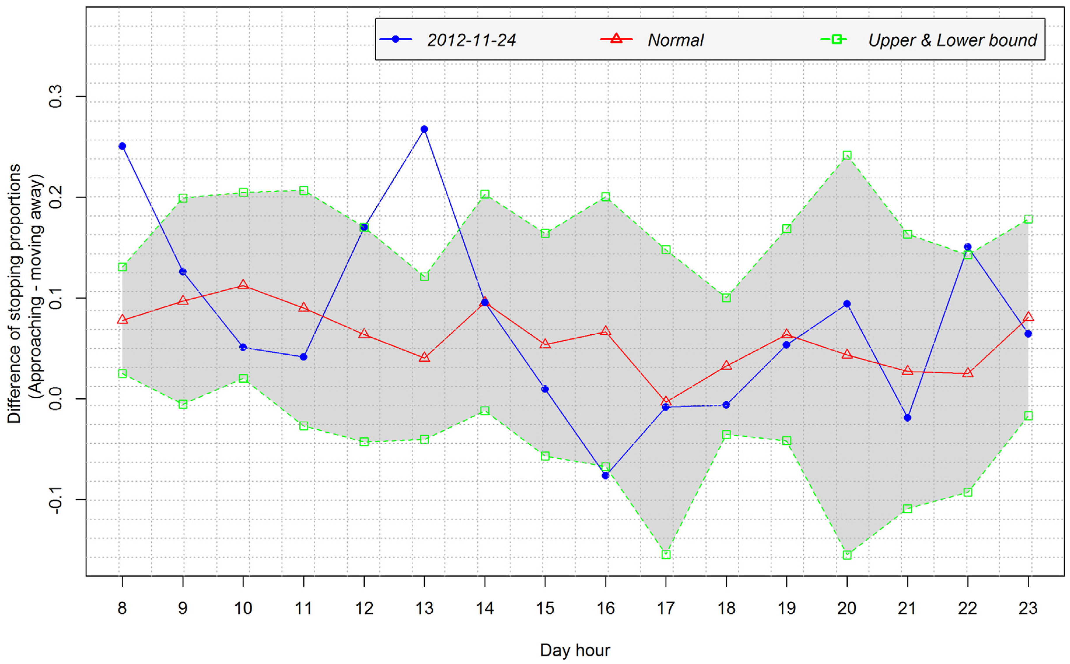
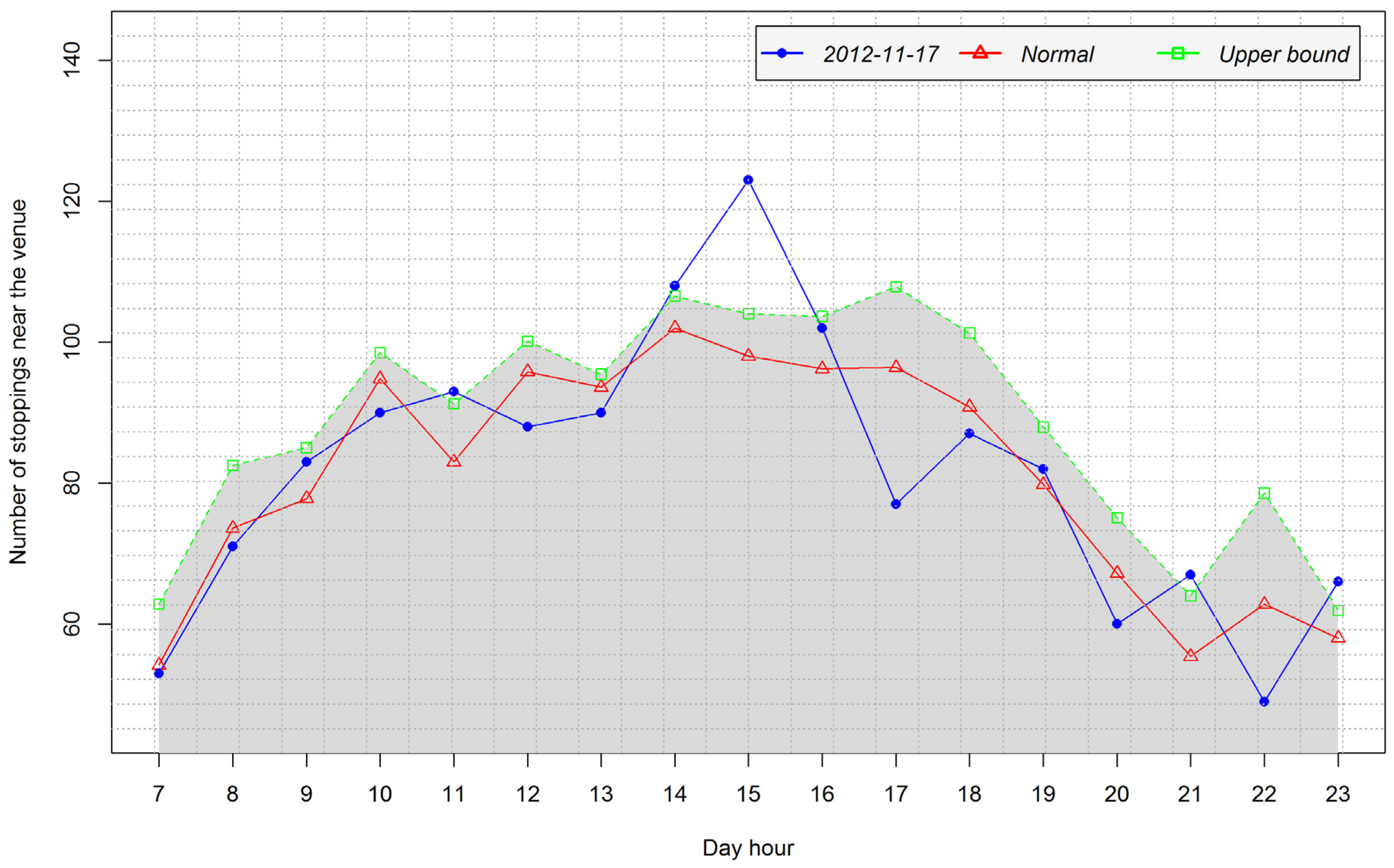
• Peak at 9:00 in the interval 8:00–11:00, peak type: −1, peak level: 0.667
• Peak at 13:00 in the interval 11:00–14:00, peak type: 1, peak level: 1
• Peak at 16:00 in the interval 15:00–18:00, peak type: −1, peak level: 1
• Peak at 20:00 in the interval 19:00–21:00, peak type: 0

By applying the method of confirming event occurrence as explained previously, the last peak is immediately rejected. The remaining three candidates form a sequence Departure-Arrival-Departure. The last two peaks in the sequence (corresponding to 13:00 and 16:00) are confirmed to be Arrival and Departure times, respectively. The intervals around these two peaks are taken as inputs to the next step for further analysis. The peak at 9:00 is an unknown case that does not indicate a big event at the stadium.

4.3.2. Analysis of Temporal Patterns of Arrival and Departure

We proceeded to conduct a local analysis at a finer temporal granularity level. To this end, we performed the same analysis on the number of stoppings near the venue (i.e., the stadium in this case). The analysis is focused on the time intervals containing the confirmed arrival and departure times. We subdivided each 1-h time interval into four sub-intervals of 15 min each. Figure 10 shows the temporal variation of the variables during smaller intervals around the arrival and departure times. This analysis allows us to refine the answer to the question of estimating the start and end times of the event assuming that the highest peak corresponds to the start or end of the event. From Figure 10a we see that the start time estimated in the previous step to be 13:00 is refined to be around 13:30. Similarly, Figure 10b shows a refinement of the end time from 16:00 to around 16:15.

The analysis further shows the temporal patterns of the arrival and departure of event attendees. The temporal pattern of arrival presented in Figure 10a shows that some event attendees have been arriving earlier before the event start time, as shown by the shorter peaks that exceed the upper bound between 11:00 and 13:00. After the start of the event (approximately after 15 min) the number of stoppings at the venue sharply dropped below the upper bound becoming almost normal. This suggests that in general event attendees arrived on time. The temporal pattern of departure shown in Figure 10b suggests that it has taken less than 30 min after the end of the event for the stoppings near the venue to return to normal, meaning that event attendees did not spend much time at the venue after the end of the event.

Different big events may show different temporal patterns of arrival and departure of attendees. For example, unlike the attendees of the event on 24 November 2012 who arrived on time and departed as soon as the event ended (see Figure 10), the attendees of the event on 14 November 2012 kept arriving after the start of the event, as shown by the number of stoppings near the venue that remained above the upper bound for some time after the peak (see Figure 11a). Attendees of the latter event also departed progressively, as shown by the number of stoppings near the venue, which remained above the upper bound during a long time interval after the peak (see Figure 11b).

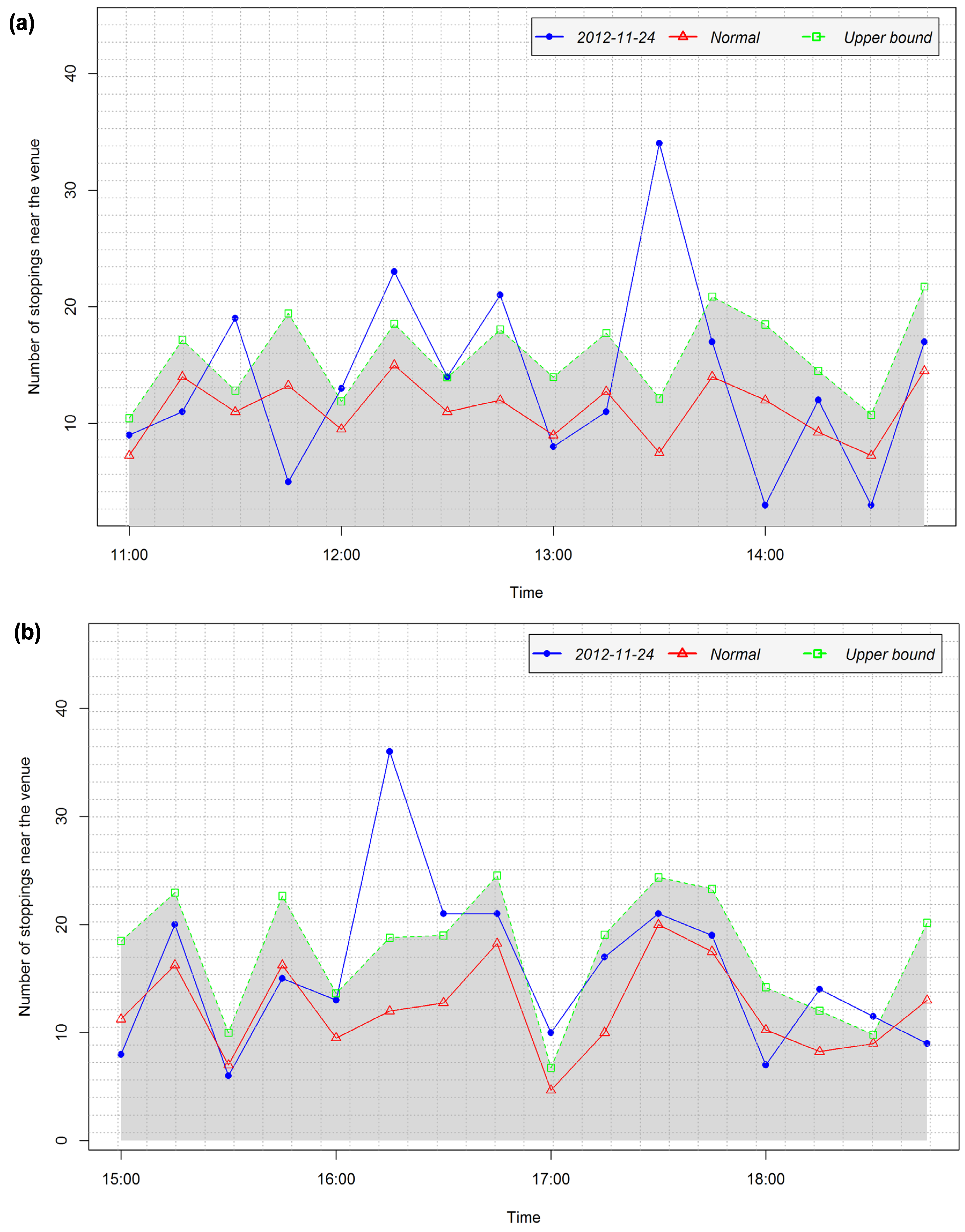
4.4. Case Study 2: Human Mobility and the Context of Medium Scale Events at the National Concert Hall

We carried out the second case study following the same steps explained in detail in Section 4.2. Because most of the events were organized at the same hour of the same day every week we could not model the normal condition for them and therefore we did not study their days. The day of 17 November 2012 on which an event was organised at a different hour (2:30 pm) compared to other days (8:30 pm) is presented here as an example of sample results. Figure 12 shows the variation of the number of bus stoppings in the neighbourhood of the venue while Figure 13 shows the variation of the balance between the number of approaching stoppings and moving-away stoppings. The candidate event occurrence time at 15:00 (see the peak in Figure 12) was confirmed to be the start of an event (see the positive peak in the corresponding uncertainty interval in Figure 13) which was refined through the analysis of the uncertainty interval at a finer granularity level (see Figure 14).

From Figure 14 we note that some event attendees arrived early (see the small peaks at around 14:15 and 14:45) but that a larger number arrived late at around 15:45. A second small peak detected at 21:00 (see Figure 12) and confirmed (see the peak at 21:00 in Figure 13) corresponds to a second event that was organised at 20:30 on the same day. As seen from Figure 12, this second event is hardly detected. Considering that at this hour the venue (almost) always has events, the cause may be the difficulty for the methodology to obtain a good model of the normal mobility pattern at this hour. It can also be due to a small number of people who moved to attend this event because of a lower importance attributed to it, or some attendees staying after attending the first event and thus not moving. Like in the first case study, we identified the absence of events (e.g., on 28 November 2012), but these results are not graphically presented here due to space constraints. Compared to the large-scale events in the first case study, a medium-scale event such as in this second case study is harder to detect fully (both the start and the end), because other mobility abnormalities in the region will highly affect the extraction of interactions.

5. Discussion

The application of the proposed methodology on real data shows that the methodology has the potential to answer questions about whether a big event occurred, estimate its start and end times, and reveal the temporal patterns surrounding the arrival and departure of event attendees. The results obtained in the experiments have been compared to the information about the occurrences of big events during the studied period (e.g., see Table 1). Although only three big events occurred in the stadium during the period we studied, the results obtained from two different case studies are promising. Two of the three events in the stadium were successfully discovered while the third was categorised as an unknown case, which needs further analysis. In the second case study, we tested two days for the occurrence of medium-scale events and found the events that occurred in one of them. In both case studies the method was able to confirm the absence of events on the event-free days.

For estimating the start and end times of the event the method considered time intervals in which the number of stoppings near the venue was exceptionally higher than its normal value. In addition, we assumed that the peak (i.e., the highest shift from the normal value) corresponds to the start or end time of the event. A comparison of the results with the ground truth (see Table 1 for example) shows that the error of this estimation is between 15 and 30 min. Considering that the events lasted at least 1 h and 30 min and that we aggregated data in time intervals of 15 min, we find this estimate acceptable and still usable.

The method performed a local analysis at a finer temporal granularity level to explore the temporal patterns of arrival and departure of event attendees. The method was able to identify attendees arriving shortly before the start of the event, despite early stiles opening, and cases where they departed progressively after the end of event, hinting at a possible on-site celebration before departure. From these temporal patterns, it is possible to discover characteristics of specific event types if more event data are available. For example, we could compare the temporal patterns associated with a rugby match (e.g., see Figure 10) with those associated with a football match (e.g., see Figure 11) and determine some specific characteristics of these two types of event. For the evaluation of these temporal patterns we explored the temporal distribution of Flickr photos taken on the days on which we detected events and Foursquare check-ins of the same period. The distribution of these data in terms of the number of items and relevant tags agreed with the results of the stadium case studies, while we found no data for the concert hall case.

A key to the successful application of the methodology is the result of the extraction of stopping interactions. This step relies on a number of parameters for detecting when the vehicle has stayed in the neighbourhood of a stop point for at least a specified amount of time. The values of these parameters have been set after a number of trials to find optimal values. However, an extended sensitivity analysis of the parameter values on a different dataset could help in setting optimal values.

We anticipate a limitation of the proposed method in regards to its ability to consider a case where another medium-scale or big event occurs around the same time in close proximity of the event venue under scrutiny (the stadium or the concert hall in our example cases). We expect that in such a case the occurrence of the other event may affect the number of stoppings attributed to the original event, making it harder to identify two times considered as arrival and departure times for the event. However, such cases where two big or medium scale events occur in a close proximity to each other and at around the same time are likely to be very rare. A general observation from the comparison of our two case studies is that the bigger the event the easier it is detected by the methodology.

Another limitation of the methodology is that it cannot be fully applied to the case of a circular route travelled always in one direction. In this case the methodology will be able to detect candidate occurrences of events, but will not be able to confirm them or do further analysis as we have described. In such a case the methodology can be supplemented by the use of social media data on which other analysis steps will be possible through the associated semantics (e.g., in titles, descriptions, and tags). Nevertheless, our methodology could play the role of restricting the search period to a small time interval.

In addition to supporting the understanding of the arrival and departure patterns of event attendees, the methodology provides some information about the effect of the event on the mobility along the route. The assumption is that the bus does not necessarily stop at every designated stop point; in most of the cases it stops only when there are passengers who need alighting or boarding. As a result, stopping at (almost) every bus stop, as may be the case at the time of an event on the route serving the event venue, is likely to cause delayed journeys. Knowing how often the bus stops and the bus stops where recurring stopping actually occurs can be useful in planning an additional line or additional buses for responding to the increased mobility demand due to the event. One problem of our study currently is that such information is provided for one bus line. We acknowledge that the methodology should cover a wider area to support larger planning issues. In this direction, the methodology can be extended by efficiently replicating the process on several bus lines. However, regarding event detection, the methodology is designed to work on large-scale events with a pre-defined location only. For small-scale events, other methods like those based on social media data [12] can be used.

To better support planning applications, the methodology needs to be improved to provide richer information. To this end, we plan to use the combination of the number and duration of stoppings and semantic information from social media data. So far we used the number of stoppings alone and tried the stopping duration as a replacement, but we found no difference in the results. We think that the combination of these two features and the semantics from social media data can provide richer information and improve the success rate of the methodology.

The advantage of our method is that it uses data of high spatial and temporal accuracy, which can be more easily collected and acquired compared to cell-phone traces or traces of private cars used in related work. Furthermore, our method performs analysis at multiple temporal granularity levels to discover global and local patterns, a feature which is very important in mobility data analysis as discussed in [1,26].

6. Conclusions and Future Work

Mobility data analysis has received important attention, but less has been done to consider the movement context. As a contribution to filling this gap, this paper proposed a methodology for integrating geographic context elements into the analysis of mobility data. The geographic context elements we considered are big events and known stop points along the route followed by the moving object. The method involves extracting three types of interaction between the moving object and the context elements: approaching the event, moving away from the event, stopping (at the event, and at a known stop point), and analysing these interactions to discover the occurrence of a big event and explore its dynamics. After testing the methodology on real data, we conclude that it can be successfully used to detect from mobility data the occurrence of a big event at a known specific place, estimate its start and end times within some error margin, and reveal the temporal patterns associated with the arrival and departure of event attendees.

The proposed methodology has the potential for applications mainly in transportation and event planning and management. As has been demonstrated by Calabrese et al. [7], the same types of events are likely to be attended by people from the same regions. We extrapolate their finding to say that these event attendees are likely to have the same behaviour regarding attending events because attendees of events of the same type from the same regions are likely to include the same people to a large degree. Therefore, the knowledge about the behaviour of attendees of an event can help in improving resource planning and usage for future events of the same type. For example, the knowledge of the relative time at which a surge of transportation need occurs and how fast event attendees leave the venue at the end of the event will help in public transportation and security control planning.

Considerations for future work include collecting a larger ground truth dataset, a detailed evaluation of the success rate of the methodology, and integrating the use of social media data to improve the success rate on event detection and widen the applicability.

References

- Dodge, S.; Weibel, R.; Ahearn, S.C.; Buchin, M.; Miller, J.A. Analysis of movement data. Int. J. Geogr. Inf. Sci. 2016, 30, 825–834. [Google Scholar] [CrossRef]
- Laube, P. Computational Movement Analysis; Springer: Berlin/Heidelberg, Germany, 2014. [Google Scholar]
- Baglioni, M.; Fernandes de Macêdo, J.A.; Renso, C.; Trasarti, R.; Wachowicz, M. Towards Semantic Interpretation of Movement Behavior. In Advances in GIScience; Sester, M., Lars, B., Volker, P., Eds.; Springer: Berlin/Heidelberg, Germany, 2009; pp. 271–288. [Google Scholar]
- Orellana, D.; Wachowicz, M. Exploring patterns of movement suspension in pedestrian mobility. Geogr. Anal. 2011, 43, 241–260. [Google Scholar] [CrossRef] [PubMed]
- Dodge, S.; Bohrer, G.; Bildstein, K.; Davidson, S.C.; Weinzierl, R.; Bechard, M.J.; Barber, D.; Kays, R.; Brandes, D.; Han, J.; et al. Environmental drivers of variability in the movement ecology of turkey vultures (Cathartes aura) in North and South America. Philos. Trans. R. Soc. Lond. B Biol. Sci. 2014. [Google Scholar] [CrossRef] [PubMed]
- Bagrow, J.P.; Wang, D.; Barabási, A.-L. Collective response of human populations to large-scale emergencies. PLoS ONE 2011, 6, e17680. [Google Scholar] [CrossRef] [PubMed]
- Calabrese, F.; Pereira, F.C.; Lorenzo, G.D.; Liu, L.; Ratti, C. The Geography of Taste: Analyzing Cell-Phone Mobility and Social Events. In Pervasive Computing; Floréeni, P., Krüger, A., Spasojevic, M., Eds.; Springer: Berlin/Heidelberg, Germany, 2010; pp. 22–37. [Google Scholar]
- Ying, J.J.; Lee, W.; Tseng, V.S. Mining geographic-temporal-semantic patterns in trajectories for location prediction. ACM Trans. Intell. Syst. Technol. 2013, 5, 1–33. [Google Scholar] [CrossRef]
- Parent, C.; Spaccapietra, S.; Renso, C.; Andrienko, G.; Andrienko, N.; Bogorny, V.; Damiani, M.L.; Gkoulalas-Divanis, A.; Macedo, J.A.; Pelekis, N.; et al. Semantic trajectories modeling and analysis. ACM Comput. Surv. 2013, 45, 42. [Google Scholar] [CrossRef]
- Spaccapietra, S.; Parent, C.; Damiani, M.L.; de Macêdo, J.A.; Porto, F.; Vangenot, C. A conceptual view on trajectories. Data Knowl. Eng. 2008, 65, 126–146. [Google Scholar] [CrossRef]
- Trasarti, R.; Olteanu-Raimond, A.-M.; Nanni, M.; Couronné, T.; Furletti, B.; Smoreda, Z.; Ziemlicki, C. Discovering urban and country dynamics from mobile phone data with spatial correlation patterns. Telecommun. Policy 2015, 39, 347–362. [Google Scholar] [CrossRef]
- Hawelka, B.; Sitko, I.; Beinat, E.; Sobolevsky, S.; Kazakopoulos, P.; Ratti, C. Geo-located Twitter as proxy for global mobility patterns. Cartogr. Geogr. Inf. Sci. 2014, 41, 260–271. [Google Scholar] [CrossRef] [PubMed]
- Pappalardo, L.; Rinzivillo, S.; Qu, Z.; Pedreschi, D.; Giannotti, F. Understanding the patterns of car travel. Eur. Phys. J. Spec. Top. 2013, 215, 61–73. [Google Scholar] [CrossRef]
- Guo, D.; Zhu, X.; Jin, H.; Gao, P.; Andris, C. Discovering Spatial Patterns in Origin-Destination Mobility Data. Trans. GIS 2012, 16, 411–429. [Google Scholar] [CrossRef]
- Andrienko, G.; Andrienko, N.; Heurich, M. An event-based conceptual model for context-aware movement analysis. Int. J. Geogr. Inf. Sci. 2011, 25, 1347–1370. [Google Scholar] [CrossRef]
- Buchin, M.; Dodge, S.; Speckmann, B. Similarity of trajectories taking into account geographic context. J. Spat. Inf. Sci. 2014, 9, 101–124. [Google Scholar] [CrossRef]
- Siła-Nowicka, K.; Vandrol, J.; Oshan, T.; Long, J.A.; Demšar, U.; Fotheringham, A.S. Analysis of human mobility patterns from GPS trajectories and contextual information. Int. J. Geogr. Inf. Sci. 2016, 30, 881–906. [Google Scholar] [CrossRef]
- Dodge, S.; Bohrer, G.; Weinzierl, R.; Davidson, S.C.; Kays, R.; Douglas, D.; Cruz, S.; Han, J.; Brandes, D.; Wikelski, M. The environmental-data automated track annotation (Env-DATA) system: Linking animal tracks with environmental data. Mov. Ecol. 2013. [Google Scholar] [CrossRef] [PubMed]
- Janssens, D.; Nanni, M.; Salvatore, R. Car traffic monitoring. In Mobility Data; Renso, C., Spaccapietra, S., Zimanyi, E., Eds.; Cambridge University Press: New York, NY, USA, 2013; pp. 197–220. [Google Scholar]
- Orellana, D.; Wachowicz, M.; Andrienko, N.; Andrienko, G. Uncovering Interaction Patterns in Mobile Outdoor Gaming. In Proceedings of the International Conference on Advanced Geographic Information Systems & Web Services (GEOWS’09), Cancun, Mexico, 1–7 February 2009; IEEE Computer Society: Washington, DC, USA, 2009; pp. 177–182. [Google Scholar]
- Dodge, S.; Weibel, R.; Lautenschütz, A.-K. Towards a taxonomy of movement patterns. Inf. Vis. 2008, 7, 240–252. [Google Scholar] [CrossRef]
- Palma, A.T.; Bogorny, V.; Kuijpers, B.; Alvares, L.O. A clustering-based approach for discovering interesting places in trajectories. In Proceedings of the 2008 ACM Symposium on Applied Computing (SAC ’08), Fortaleza, Ceara, Brazil, 16–20 March 2008; ACM Press: New York, NY, USA, 2008. [Google Scholar]
- Dublinked: Dublin Bus GPS sample data from Dublin City Council (Insight Project). Available online: https://data.dublinked.ie/dataset/dublin-bus-gps-sample-data-from-dublin-city-council-insight-project (accessed on 11 April 2016).
- An Garda Síochána, Ireland’s National Police Service. Available online: http://www.garda.ie/News/default.aspx (accessed on 15 March 2016).
- ISSUU. The National Concert Hall Sept-Nov 2012 Calendar of Events. Available online: https://issuu.com/nationalconcerthall/docs/sept-nov2012calendar (accessed on 20 November 2016).
- Laube, P.; Purves, R.S. How fast is a cow? Cross-Scale Analysis of Movement Data. Trans. GIS 2011, 15, 401–418. [Google Scholar] [CrossRef]