Abstract
A multivariate Bayesian spatial modeling approach was used to jointly model the counts of two types of crime, i.e., burglary and non-motor vehicle theft, and explore the geographic pattern of crime risks and relevant risk factors. In contrast to the univariate model, which assumes independence across outcomes, the multivariate approach takes into account potential correlations between crimes. Six independent variables are included in the model as potential risk factors. In order to fully present this method, both the multivariate model and its univariate counterpart are examined. We fitted the two models to the data and assessed them using the deviance information criterion. A comparison of the results from the two models indicates that the multivariate model was superior to the univariate model. Our results show that population density and bar density are clearly associated with both burglary and non-motor vehicle theft risks and indicate a close relationship between these two types of crime. The posterior means and 2.5% percentile of type-specific crime risks estimated by the multivariate model were mapped to uncover the geographic patterns. The implications, limitations and future work of the study are discussed in the concluding section.
1. Introduction
Ecological studies of crime are of great interest to geographers and criminologists as they can reveal the geographic pattern of crime risks as well as the relevant risk factors explaining that pattern. Researchers have used non-spatial regression models in crime analysis. For example, Craglia et al. [1] adopted a standard logistic regression model to explore the relationship between socioeconomic characteristics and high-intensity crime areas. Such non-spatial models assume that the observations are independent and identically distributed. This assumption, however, is usually problematic in empirical crime studies. In practice, adjacent areas often have similar crime data, i.e., crime data are very likely to be spatially auto-correlated, especially at small-area scales as often indicated by clusters appearing on crime maps. Ignoring this spatial dependence in ecological studies can result in estimates with underestimated standard errors [2]. Thus, methodologically, the traditional non-spatial models are inappropriate to analyze crime at the small-area level.
Spatial autocorrelation is typically modeled using the spatial lag model [3], the spatial error model [4] or other frequentist statistical models [5] in crime analysis. However, there are limitations with frequentist models. The spatial lag and error models [6] can only be used to model continuous variables (i.e., outcomes of rates, not counts) following a normal distribution. In addition, frequentist spatial models cannot process available information systematically [7]. These approaches are also incapable of dealing with the small number problem, which may produce unreliable risk estimations if not accounted for in the model [8].
The limitations of the frequentist models in small-area crime analysis can be overcome by Bayesian spatial models. Bayesian statistics, unlike frequentist statistics, treats unknown parameters as random variables expressed in terms of probabilities. It combines prior knowledge and observation data to obtain posterior distributions for parameters of interest. The implementation of Markov chain Monte Carlo (MCMC) methods and software such as WinBUGS to implement MCMC [7,9] make it possible to fit complex spatial models. Although Bayesian spatial models can tackle problems encountered in frequentist approaches, and thus are advantageous in small-area analysis, they are still seldom applied in crime studies. This is changing, however, as more researchers have become aware of the advantages of Bayesian spatial models. A small but growing body of research has adopted Bayesian spatial modeling approaches in crime analysis [10,11,12,13,14,15,16,17]. For example, researchers using Bayesian spatial models have investigated contextual influences on domestic violence [12,15,18], juvenile offenders [14] and property crime [13].
The existing criminological research conducted by using Bayesian spatial models typically focuses on one type of crime. In these applications, the modeling methods adopted are univariate in nature. Counts of different types of crime can be interrelated and are multivariate to some extent as the crimes may share some missing or unmeasured variables. Modeling interrelated crime counts by aggregating them all together or separately using a univariate approach for each crime type fails to recognize this correlation and may ignore information shared in those missing variables. In ecological analysis, ignoring correlation structures between outcomes may distort the estimates of regression coefficients and result in biased and inefficient parameter inferences [19]. Nonetheless, to the best of our knowledge, there has been little work on multivariate Bayesian crime modeling in criminological research.
This paper uses a multivariate Bayesian spatial modeling approach to jointly model the counts of two types of crime, i.e., burglary and non-motor vehicle theft, and explore the geographic pattern of crime risks at a small-area scale. Burglaries and non-motor vehicle thefts can be interrelated as they belong to the same theft category in China and may share some omitted variables. The multivariate Bayesian spatial model takes into consideration the correlation between these two types of crime. This is of both theoretical and practical importance. From the theoretical perspective, there are gains in precision and efficiency of estimates through this joint modeling method achieved by pooling all the available data from different crime sources. Multivariate Bayesian models can take advantage of correlations across different types of crime. In addition, the multivariate spatial model provides information not only on similarities but also on differences in the effects of covariates on crimes. The model could also be used to identify crime-specific risk factors. From a practical perspective, both burglaries and non-motor vehicle thefts are common and have a high incidence in China. Police departments and the public are greatly concerned about these two types of crime and are interested in identifying relevant risk factors. The information gained from the joint analyses could help develop a greater understanding of the spatial distribution and determinants of crimes, contributing to more efficient and effective crime intervention and prevention strategies. Through the joint multivariate crime modeling approach, these issues can be addressed in a unified framework.
The remainder of this manuscript is organized in the following manner. First, we briefly describe the study region and relevant data. Next, we explain the multivariate Bayesian spatial modeling approach in detail. Third, results of the analysis are shown, followed by a discussion of the results. The strengths and limitations of the study, as well as directions for feature research are concluded in the final section.
2. Study Region and Data
2.1. Study Region
This study was carried out in Jianghan District, Wuhan, China. Wuhan, the largest city in Central China, is an important industrial base and transportation hub. The Jianghan District of Wuhan lies at the intersection of the Yangtze River and the Han River. It is the most prosperous and populated urban district in the city. The neighborhood was the unit of analysis in the current research. It is a direct sublevel of a sub-district, which is one of the smallest political divisions in China. The Jianghan District consists of 116 neighborhoods; two neighborhoods were excluded from the study because of missing data.
2.2. Data
Data on burglaries and non-motor vehicle thefts came from the city’s 110-reporting system managed by Wuhan Public Security Bureau. The 110-reporting system is the primary source of official crime information in China, as 110 is the emergency telephone number for the public to report crimes and emergencies to police. A total of 1747 burglaries and 2341 non-motor vehicle thefts occurred in the study region from 1 January 2015 to 31 December 2015, respectively. Both types of incidents were unevenly distributed among neighborhoods (see Table 1). We used these incident data as dependent variables.

Table 1.
Descriptive statistics of the dependent and independent variables.
Independent variables were selected based on social disorganization theory [20] and routine activity theory [21]. Social disorganization theory suggests that crime levels in neighborhoods are strongly correlated with local ecological characteristics. Socioeconomic stress can decrease social organization. Socially disorganized neighborhoods have lower levels of social control, which will decrease the monitoring of criminal activity and further lead to occurrences of crime [22,23]. Routine activity theory identifies three elements necessary for a crime: motivated offenders, suitable targets, and the absence of capable guardians [24,25]. If any of these is missing, a crime will be less likely to occur. According to these two theories, six variables at the neighborhood level were assumed to be potential risk factors. They were population density, unemployment rate, percentage of highly educated, percentage of young males, policing and bar density.
Population density was measured by the number of residents per square kilometer. It was included to control for differences in neighborhood sizes and populations [26,27]. It is generally believed that a larger population density usually leads to a higher crime rate [28,29]. However, higher population density also increases street monitoring by residents [30], deterring anyone from committing crime.
Unemployment rate was calculated as the number of unemployed residents between ages 18–60 divided by the number of all the residents within the same age range in the neighborhood. It is usually believed that unemployment rate is positively related to crime and researches have used it as one indicator of socioeconomic status [14,31,32]. Percentage of highly educated was the percentage of population age 20 or older with a high school diploma or equivalent. This variable is also often used to measure economic deprivation [14,32,33]. Therefore, in our analysis, the unemployment rate and percentage of highly educated were used as a proxy for socioeconomic status. Neighborhoods with a high unemployment rate and a low percentage of highly educated inhabitants, relatively speaking, likely have a lower socioeconomic status. According to social disorganization theory [20], there is often a positive correlation between low socioeconomic status and crime.
Percentage of young males referred to the percentage of males between ages 15–24. This factor was considered because previous research has shown that young males are hugely overrepresented among those engaged in criminal activities [23,34,35].
Policing was measured by the number of community policing and monitoring rooms in each neighborhood per 10,000 people. Policing rooms are set up by local police stations and staffed by several police officers to guarantee neighborhood’s security. The relationship between policing and crime has been investigated in previous studies [15,27].
Bar density was defined as the number of bars per 10,000 people in each neighborhood. We included this land-use variable in the analysis to test if it could explain the spatial pattern of crime risks. Researchers have long been interested in land-use variables in crime analysis [36,37].
Descriptive statistics, including minimum, maximum, mean and standard deviation (SD) of the dependent and independent variables at the neighborhood level are shown in Table 1.
Table 2 summarizes the correlation matrix of the six independent variables. This table indicates that the pair of population density and unemployment rate had the most significant correlation coefficient (0.420). According to Evans [38], this correlation level is moderate while those of other pairs of variables are weak or very weak. Therefore, we did not consider the multicollinearity issue and used all six variables in the modeling.
Table 2.
Correlation matrix of the independent variables.
3. Methods
3.1. Modeling Framework
The dependent variable was the number of crimes by type, assumed to follow a Poisson distribution:
where k refers to the type of crime, is the observed number of crimes of the type k in neighborhood i, is the expected value of the Poisson distribution, is the number of crimes that could be expected, and is the corresponding area-specific and type-specific crime risk. In our Bayesian spatial modeling approach, the logarithm of the expected value was linked to the independent variables:
where is an offset term for crime type k in neighborhood i with the regression coefficient being one, is the intercept for crime type k, , , are the observations of the independent variables in neighborhood i, , , are the corresponding regression coefficients for crime type k, is an unstructured random effects term to account for the overdispersion that may arise when small-area count data are modeled, and is a spatially structured random effects term to account for spatial autocorrelation.
3.2. Prior Specification for the Univariate Model
In order to fully express the multivariate Bayesian spatial model, we describe prior specifications used in the univariate model and contrast them to their multivariate counterparts. Prior specification for unknown parameters is important in Bayesian inference as posterior distributions of parameters are deduced by combing prior knowledge and data. was assigned a uniform prior dflat() due to a sum-to-zero constraint on the random effects [39]:
, the regression coefficient, was specified to follow a non-informative normal distribution with a mean of zero and a variance of 10,000 as we had no genuine prior expectations for direction and magnitude of the independent variable’s effect:
The univariate Bayesian spatial model ignores correlations across different types of crime as it assumes that the random effects for different types of crime are independent. In the case of the univariate model, was specified as an independent normal distribution with an expected mean of zero and a variance of :
, the spatially structured random effects term, was determined through an intrinsic conditional autoregressive (ICAR) distribution that is widely used in spatial statistics [40,41]. Under the ICAR specification, this will result in:
where , if i and j are adjacent and otherwise 0, and is the number of neighborhoods adjacent to neighborhood i. Specifically, according to the specification of the ICAR model, the conditional distribution of given the remaining components () is normal with mean and variance . The variation of is controlled by the overall variance parameter .
Regarding hyperparameters and , the reciprocals of these two parameters were assumed to follow a commonly used Gamma distribution [42]:
The WinBUGS code for the univariate model can be found in the Supplementary Materials.
3.3. Prior Specification for the Multivariate Model
The specifications from Equation (4) to Equation (9) are essentially equivalent to the specifications of the univariate Poisson spatial model for each crime type, i.e., burglary and non-motor vehicle theft, respectively. However, these specifications provide the possibility of being directly comparable with the multivariate joint specifications.
The prior specifications of and for the multivariate Bayesian spatial model were the same as those for the univariate model. In contrast to the univariate model assuming that the random effects for different types of crime are independent, the multivariate model takes account of correlations across random effects. Therefore, the main differences between the multivariate model and the univariate model are the prior specifications of the random effects. For the multivariate spatial model, was assumed to follow a multivariate normal distribution:
where is a vector with all elements zeroes and is the covariance matrix estimated by a Wishart distribution:
where and are the scale matrix and the degrees of freedom, respectively. For computational convenience, the Wishart distribution is commonly used as it is the conjugate prior for the inverse of the covariance parameters of multivariate normal distributions [43,44]. The scale matrix, , is often set to be a scaled identify matrix with a scaling factor (see [45,46,47], for example). In our analysis, we chose 0.01 as the scaling factor, i.e., setting ’s diagonal entries to , a specification adopted to run sensitivity analysis for the precision matrix of a multivariate normal distribution [45]. The parameter , the degrees of freedom, was set equal to 2 in order to make the prior on minimally informative [48,49].
As to the spatially structured random effects , the ICAR specification in the univariate model extends naturally to a multivariate ICAR specification by replacing the univariate normal conditional distribution with a multivariate conditional distribution:
where is the mean vector , and is the covariance matrix, respectively. As in the univariate case, if i and j are adjacent and 0 otherwise, and is the number of neighbors of neighborhood i. Diagonal elements of , i.e., and , are the conditional variances of and respectively, and off-diagonal elements, i.e., and , represent the conditional within-neighborhood covariance between and . This specification of gives the multivariate equivalent of the standard ICAR specification [40]. The multivariate ICAR model is building on multivariate conditional autoregressive (MCAR) models described by Mardia [50]. It is the intrinsic version of the Multivariate Conditional Autoregressive (MCAR) model [51] and has been used in spatial analysis [46,52]. Similar to the specification of , we adopted the same approach to determine ; a Wishart distribution was chosen for its inverse [45,48,49]:
where and are the scale matrix and the degrees of freedom, respectively.
The WinBUGS code for the multivariate model can be found in the Supplementary Materials.
3.4. Model Implementation and Assessment
Models were fitted by the MCMC simulation approach in WinBUGS 1.4.3. Before they were fitted, all independent variables were standardized (centered around the mean and then divided by the standard deviation) to improve convergence [51]. For each model, two parallel sampling chains with different initial values were run. We evaluated the convergence of each model by visual inspection of the trace plots and the Gelman-Rubin convergence statistic [53]. Convergence occurred after the first 50,000 iterations. Each chain was run for a further 100,000 iterations, generating 200,000 samples with acceptable Monte Carlo errors (<5% of the posterior standard deviation) for posterior estimations. We assessed different models using the deviance information criterion (DIC) [54]. Broadly, DIC is a generalization of Akaike Information Criterion [55] and it is defined as:
where is the posterior mean of the deviance and is the number of effective parameters in the model. DIC takes both model fit (summarized by ) and model complexity (captured by ) into consideration when comparing models. Smaller values of DIC suggest better-fitting models.
4. Results
4.1. Comparison of the DICs
Table 3 presents the results of the univariate and the multivariate regression models fitted in WinBUGS. Both models included an unstructured random effects term and a spatially structured random effects term. The major difference is the way in which the random effects were specified; one is in the univariate form, while the other is in the multivariate form. The univariate model had a DIC of 1344.709; when extended to the multivariate model, the DIC dropped to 1325.992, a difference of 18.717. This difference in DICs can be explained by the posterior deviance and the number of effective parameters . The for the multivariate model was 1145.07, as compared to 1150.30 for the univariate model. The higher for the univariate model indicates a poor fit relative to the fit of the multivariate model. The in the univariate model was 194.409, while extending the univariate random effects to the multivariate form made 13.487 points lower. This reduction in indicates that the random effects might be correlated. Indeed, once the correlation between random effects was considered in the multivariate model, the dropped, largely explaining the improvement in DIC. In short, the multivariate model was more parsimonious than the univariate alternative. A model with a better fit and fewer parameters is always preferred. Therefore, in terms of DIC, the overall model comparison criterion that takes into account both model fit and model complexity, the multivariate model was better suited to our data. We studied the sensitivity of the results to the choice of hyperparameters. Regarding the univariate model, we note that standard deviation uniform priors are now commonly used [56]. Thus, we used a non-informative uniform hyperprior distribution dunif(0,100) for the standard deviation parameters of and [16]. It yielded a DIC with a difference of 5.077 (1349.786 versus 1344.709). For the multivariate model, we selected the two-dimensional identity matrix, an uninformative prior often used in practice, for and [45,47]. It yielded a DIC with a difference of 4.198 (1330.190 versus 1325.992). The sensitivity analysis suggests that the results of the univariate and the multivariate models were both not overly sensitive to the selected hyperprior specifications.
Table 3.
Results of the univariate and the multivariate models.
4.2. Analysis of Risk Factors
Regarding the independent variables, population density and bar density had a clear association with both types of crime at the 95% credible interval (CI) in both the univariate model and the multivariate model. The other four variables, i.e., the unemployment rate, percentage of highly educated population, percentage of young males and policing, were not significant for the two types of crime in both models. The univariate model and the multivariate model identified the same set of significant variables for both crimes. However, the precisions of all the regression coefficients from the univariate model were overestimated as compared to those from the multivariate model. Overall, the regression coefficients were much changed after extending the univariate random effects to their multivariate counterparts. This indicates that the correlation between burglaries and non-motor vehicle thefts had a great effect on coefficient estimates. Since the multivariate model better fit the data, our analyses are based on this model.
Population density had a negative effect on both types of crime. Bar density was found to be positively correlated with both burglaries and non-motor vehicle thefts at the 95% CI. Generally, holding all other variables constant, the relative risk of burglary and non-motor vehicle theft will decrease by 28.12% and 41.32%, respectively, with an increase of one standard deviation in population density (Equations (15) and (16)).
Using the same calculation method, we estimated that the relative risk of burglary and non-motor vehicle theft will increase by 67.30% and 46.96%, with an increase of one standard deviation in bar density, respectively (Equations (17) and (18)).
4.3. Correlation between the Random Effects
Table 4 shows the posterior means of the covariance/correlation matrix of the random effects. Although the correlation between the unstructured random effects was low (0.1398), the correlation between the spatially structured random effects was high (0.7664). Possibly due to the dominance of the spatially structured random effects, the posterior correlation between the total random effects was also high (0.7953), indicating the close relationship between the two types of crime in the data. As a consequence, like any statistical model, this correlation needs to be incorporated into the estimation. In the multivariate model, by calculating the inner product of the two crime risks, the mean and the standard deviation of type-specific crime risks, we further computed the correlation between the crime risks. The posterior mean of the correlation was 0.7592, again suggesting a strong shared geographical pattern of risks between burglaries and non-motor vehicle thefts.
Table 4.
Posterior covariance/correlation matrix of the random effects: upper triangle, covariance of the random effects; lower triangle, correlation of the random effects.
4.4. Mapping the Relative Risks
The posterior mean risks of burglary and non-motor vehicle theft estimated by the multivariate model are shown in Figure 1a and Figure 1b, respectively. In contrast to the standardized crime ratio (SCR), a measure of relative risks obtained by dividing the observed number of crime incidents to the expected number, the risks shown in Figure 1 were estimated while accounting for the effects of the independent variables, the unstructured random effects, and the spatially structured random effects. No neighborhood was assigned a risk value of exactly zero in Figure 1, although the SCRs of some neighborhoods would be zero as no crimes occurred in these neighborhoods. This difference between the SCRs and the risks shown in Figure 1 was mainly due to the spatial smoothing effect from the spatially structured multivariate random effects. The multivariate model can borrow strength not only from the estimates of the other crime type in the same neighborhood but also through the spatial correlation, from those in the adjacent neighborhoods. This “borrowing strength” effect helps stabilize risk estimations.
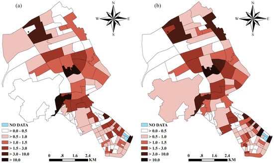
Figure 1.
The posterior mean risks of (a) burglary and (b) non-motor vehicle theft estimated by the multivariate model.
In terms of the type-specific relative risks, Figure 1a indicates that three neighborhoods had a burglary risk value higher than 10.0 and 38 neighborhoods had a risk value greater than 1.0. With regard to non-motor vehicle theft, there were also three neighborhoods with a risk value higher than 10.0 as can be seen from Figure 1b. In addition, 43 neighborhoods had a non-motor vehicle theft risk greater than 1.0. Taken together, two neighborhoods had both crime risks higher than 10.0. About 25.44% of all the neighborhoods (29 out of 114 neighborhoods) had both crime risks greater than 1.0, indicating they had crime risks higher than the average for the whole study region.
In addition to the posterior means, we also mapped the 2.5% percentile of the posterior distribution of (Figure 2). Percentiles of the posterior distribution of parameters of interest are useful in interpreting the results of a Bayesian analysis. In the current study, the 2.5% percentile provided valuable information about the pattern of crime risks. The different shadings shown in Figure 2 refer to the value of such that 97.5% of its simulated values were greater than the specified value. Figure 2a shows that there were 18 neighborhoods with a posterior 2.5% percentile value of burglary risk great than 1.0. Of particular note is that the percentile value in two neighborhoods was higher than 10.0. Figure 2b indicates that there were 23 neighborhoods having the 2.5% percentile value of non-motor vehicle theft risk greater than 1.0, and one neighborhood having a percentile value greater than 10.0. In short, nine neighborhoods had the 2.5% percentile values of both burglary risk and non-motor vehicle theft risk greater than 1.0 and one neighborhood had percentile values higher than 10.0 for both types of crime. These neighborhoods need to be further investigated by researchers and should be given adequate attention by the relevant authorities.
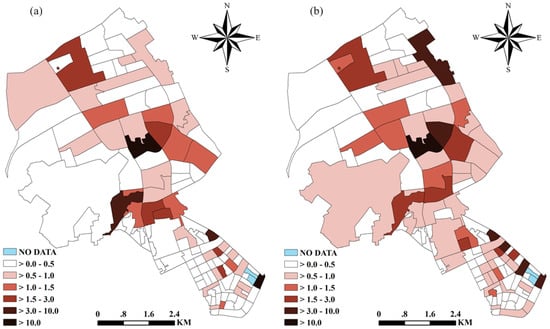
Figure 2.
The 2.5% percentile of the posterior distribution of (a) burglary risks and (b) non-motor vehicle theft risks estimated by the multivariate model.
5. Discussion
This research applied a multivariate Bayesian spatial modeling approach to jointly model the counts of burglaries and non-motor vehicle thefts and estimate the relative risks of these two types of crime at a small-area scale. The multivariate model accounts for the correlation between different types of crime. This correlation cannot be recognized when separate univariate models are estimated for each crime type. Although the univariate model identified the same set of significant covariates for both crimes as the multivariate model did, a smaller DIC for the multivariate spatial model suggests that it was better supported by our data (Table 3). In addition, the precisions of all the regression coefficients from the univariate model were overestimated as compared to those from the multivariate model (Table 3). Therefore, the multivariate model is superior to the univariate model.
Our analyses show that population density and bar density had a clear association with both types of crime in both the univariate and the multivariate models (Table 3). Population density was negatively correlated with both crime risks. The clear association between population density and crime found in the present study is in accordance with other studies showing that residential density can lower crime rates [26,27]. This may be due to the closer and easier street monitoring possible when there is a larger population density [30]. Burglary and non-motor vehicle theft risks were higher in neighborhoods that had more than the average bar density. The linkage between bars and crimes is generally supported in the literature [57]. The unemployment rate and percentage of highly educated were not significantly related to both types of crime in either model. This is somewhat unexpected as it is not in accordance with social disorganization theory. One possible reason may be that these two variables cannot fully represent socioeconomic status. Issues regarding the ecological fallacy [58,59] and the modifiable area unit problem [60] also warrant consideration. However, similar results have been found in an analysis of other crime data [32]. Policing did not have a clear association with both types of crime. This is not in line with Faria et al. [27], who found that there was a positive relation between policing and burglaries. Nevertheless, our results are not entirely unexpected. Policing can prevent crime but a larger policing presence is typically a reaction to high crime areas. Therefore, there may not be a clear association between policing and crime.
Through the joint modeling of burglaries and non-motor vehicle thefts, our results suggest that there was a tight relationship between the two types of crime (Table 4). The correlation between the relative risks of the two crimes was high (0.7592), indicating a strong shared geographical pattern of risks between burglaries and non-motor vehicle thefts.
We mapped the means (Figure 1) and the 2.5% percentile (Figure 2) of the posterior distribution of crime risks estimated by the multivariate Bayesian spatial model. By demonstrating the spatial distribution of crime risks and highlighting areas with high crime risks, the maps shown in Figure 1 and Figure 2 provide a scientific basis for policy formulation and resource allocation.
We note that some other models, such as the shared component model and the smoothed analysis of variance (SANOVA) model, may also be used to jointly model different types of crime. The shared component model can separate the underlying risk surface for each crime into a shared and a crime-specific component [61]. However, when the shared component model is extended to the joint analysis of more than two types of crime, the number of possible permutations of shared and specific components may rapidly become prohibitive [61]. Moreover, the interpretation of a shared component in such cases is more difficult [51]. The SANOVA model is also capable of modeling a multivariate outcome [62,63,64]. According to this model, a series of orthogonal contrasts (in the sense of analysis of variance) is considered [63]. The choice of these contrasts is a main problem with the SANOVA model, as the degree of benefit obtainable through fitting the model mainly depends upon how appropriate this choice is, and often there are no clear standards and criteria to help choose them [64]. The multivariate ICAR model adopted in our analysis is a natural extension of the commonly used ICAR model in univariate studies. It can easily be extended to the joint analysis of three or more types of crime.
6. Conclusions
Our study represents a contribution to the existing criminological literature as the multivariate Bayesian spatial modeling approach is seldom used in crime analysis. In contrast to the univariate model, the multivariate Bayesian spatial model not only takes into account correlations across different types of crime in the same spatial unit but also takes advantage of its neighbors to borrow strength. This “borrowing strength” effect can overcome the small number problem and contributes to stable risk estimations.
The results of our study have practical implications. The use of the multivariate Bayesian spatial modeling approach provides a new perspective to better understand the risk factors associated with different types of crime (Table 3) as well as the relation between crimes (Table 4). It can highlight areas with high crime risks (Figure 1 and Figure 2) and therefore provides a scientific basis for crime prevention and intervention strategies. Generally, police in charge of burglaries and non-motor vehicle thefts in the Jianghan District should focus on neighborhoods that have a high bar density. In addition, neighborhoods showing the highest crime risks should be given adequate attention more generally. A further investigation, identifying environmental exposures specific to these parts of the Jianghan District showing a high crime risk, may be worthwhile. This helps identify other features of the neighborhood context to explain high levels of risk and thus can be used for a better targeted prevention and intervention efforts. Additionally, as our analysis was conducted at a small-area scale, it can inform an efficient use of resources. Rather than allocate resources through larger areas such as sub-districts, understanding the distribution of crime risks at the neighborhood level will facilitate more precise targeting of resources such that they are used most efficiently and effectively.
This study also has some limitations. First, our crime data were obtained from the city’s 110-reporting system. Flaws in the data, such as data entry errors and the issue of missing data related to non-reporting of crimes, have been acknowledged [65]. However, despite these limitations, the 110-reporting system does provide the most authoritative source of crime information in China. Second, we used residential population as the at-risk population to calculate expected crime counts. We did not take into account daytime changes in population size due to commuting. This may influence the risk estimations and bias the assessment of contextual influences on crime risks in ecological crime studies as indicated by recent research [66,67,68,69]. Third, the measures used to represent socioeconomic status (i.e., the unemployment rate and percentage of highly educated) may not be powerful enough, as other related variables, such as average household income [27], percentage of individuals below the poverty line [70] and percentage of high occupational status [14], were not included. In addition, socioeconomic status is only one indicator of social disorganization. Other indicators commonly used to operationalize social disorganization include ethnic heterogeneity, family disruption, socioeconomic status and residential mobility [4,33]. However, due to unavailability of data, these indicators are not included in our analysis. Another limitation of the study is that we did not account for the role of the spatial configuration in explaining crime risks. Recent research has shown that spatial configuration can be a substantial factor in creating crime risks and in revealing the sources of spatial autocorrelation in crime data [71].
Despite the limitations, we would like to emphasize that the main purpose of our paper is to present and illustrate a multivariate Bayesian spatial model. Previous crime data are often analyzed by modeling each crime type separately without accounting for correlations that may exist among different types of crime. The multivariate model presented in the current research can cope with both the correlation structure and overdispersion in the crime data. It acknowledges dependence between different types of crime as well as dependence across space. In addition, this model can easily be extended to jointly analyze more than two types of crime.
There are several important avenues for future work. First, additional tests of the multivariate model with different crime data are recommended. Second, the current multivariate model should be extended to incorporate more than two types of crime to deepen our understanding of crime patterns and the correlations among different crimes. Third, future research should fully investigate if spatial configuration is a relevant variable in spatial models of urban crime as this is an often under evaluated topic in crime data modeling. Fourth, as shown by Helbich and Jokar Arsanjani [72], crime patterns change over time. It is advisable to collect more years of crime data and extend the multivariate spatial model into a spatio-temporal one to analyze the change of crime patterns over years.
Supplementary Materials
The following are available online at www.mdpi.com/2220-9964/6/1/16/s1. The WinBUGS code for the univariate and the multivariate models.
Acknowledgments
The authors thank Wuhan Public Security Bureau for providing data for the research. This study was supported by a Grant for Key Research Program from China’s Ministry of Public Security (Grant No. 2013022DYJ018), the National Science and Technology Pillar Program (Grant No. 2012BAH35B03) and LIESMARS Special Research Funding. The authors are grateful for the valuable comments and suggestions from anonymous reviewers.
Author Contributions
Hongqiang Liu and Xinyan Zhu worked together. Hongqiang Liu conceived of the idea, designed the experiment, carried out the experiment, analyzed the results and drafted the manuscript. Xinyan Zhu provided suggestions for the writing and edited the manuscript. Both authors have read and approved the final manuscript.
Conflicts of Interest
The authors declare no conflict of interest.
References
- Craglia, M.; Haining, R.; Signoretta, P. Modelling high-intensity crime areas in english cities. Urban Stud. 2001, 38, 1921–1941. [Google Scholar] [CrossRef]
- Law, J.; Haining, R. A bayesian approach to modeling binary data: The case of high-intensity crime areas. Geogr. Anal. 2004, 36, 197–216. [Google Scholar] [CrossRef]
- Morenoff, J.D.; Sampson, R.J.; Raudenbush, S.W. Neighborhood inequality, collective efficacy, and the spatial dynamics of urban violence. Criminology 2001, 39, 517–558. [Google Scholar] [CrossRef]
- Andresen, M.A. A spatial analysis of crime in Vancouver, British Columbia: A synthesis of social disorganization and routine activity theory. Can. Geogr. 2006, 50, 487–502. [Google Scholar] [CrossRef]
- Stein, R.E.; Conley, J.F.; Davis, C. The differential impact of physical disorder and collective efficacy: A geographically weighted regression on violent crime. GeoJournal 2016, 81, 351–365. [Google Scholar] [CrossRef]
- Anselin, L. Spatial Econometrics: Methods and Models; Kulwer Academic: Dordrecht, The Netherlands, 1988; Volume 4. [Google Scholar]
- Carlin, B.P.; Louis, T.A. Bayes and Empirical Bayes Methods for Data Analysis, 2nd ed.; Chapman and Hall: London, UK, 2000. [Google Scholar]
- Gelman, A.; Price, P.N. All maps of parameter estimates are misleading. Stat. Med. 1999, 18, 3221–3234. [Google Scholar] [CrossRef]
- Spiegelhalter, D.J.; Thomas, A.; Best, N.G.; Gilks, W.R. Bugs: Bayesian Inference Using Gibbs Sampling, Version 0.50; MRC Biostatistics Unit, Cambridge University: Cambridge, UK, 1995. [Google Scholar]
- Haining, R.; Law, J. Combining police perceptions with police records of serious crime areas: A modelling approach. J. R. Stat. Soc.: Ser. A (Stat. Soc.) 2007, 170, 1019–1034. [Google Scholar] [CrossRef]
- Freisthler, B.; Weiss, R.E. Using bayesian space-time models to understand the substance use environment and risk for being referred to child protective services. Subst. Use Misuse 2008, 43, 239–251. [Google Scholar] [CrossRef] [PubMed]
- Cunradi, C.B.; Mair, C.; Ponicki, W.; Remer, L. Alcohol outlets, neighborhood characteristics, and intimate partner violence: Ecological analysis of a California city. J. Urban Health 2011, 88, 191–200. [Google Scholar] [CrossRef] [PubMed]
- Law, J.; Chan, P.W. Bayesian spatial random effect modelling for analysing burglary risks controlling for offender, socioeconomic, and unknown risk factors. Appl. Spat. Anal. Policy 2012, 5, 73–96. [Google Scholar] [CrossRef]
- Law, J.; Quick, M. Exploring links between juvenile offenders and social disorganization at a large map scale: A bayesian spatial modeling approach. J. Geogr. Syst. 2013, 15, 89–113. [Google Scholar] [CrossRef]
- Gracia, E.; López-Quílez, A.; Marco, M.; Lladosa, S.; Lila, M. Exploring neighborhood influences on small-area variations in intimate partner violence risk: A bayesian random-effects modeling approach. Int. J. Environ. Res. Public Health 2014, 11, 866–882. [Google Scholar] [CrossRef] [PubMed]
- Law, J.; Quick, M.; Chan, P. Bayesian spatio-temporal modeling for analysing local patterns of crime over time at the small-area level. J. Quant. Criminol. 2014, 30, 57–78. [Google Scholar] [CrossRef]
- Law, J.; Quick, M.; Chan, P.W. Analyzing hotspots of crime using a bayesian spatiotemporal modeling approach: A case study of violent crime in the greater toronto area. Geogr. Anal. 2015, 47, 1–19. [Google Scholar] [CrossRef]
- Gracia, E.; López-Quílez, A.; Marco, M.; Lladosa, S.; Lila, M. The spatial epidemiology of intimate partner violence: Do neighborhoods matter? Am. J. Epidemiol. 2015, 182, 58–66. [Google Scholar] [CrossRef] [PubMed]
- Congdon, P. Bayesian Statistical Modelling, 2nd ed.; John Wiley & Sons: West Sussex, UK, 2007. [Google Scholar]
- Shaw, C.R.; McKay, H.D. Juvenile Delinquency and Urban Areas; University of Chicago Press: Chicago, IL, USA, 1942. [Google Scholar]
- Cohen, L.E.; Felson, M. Social change and crime rate trends: A routine activity approach. Am. Sociol. Rev. 1979, 44, 588–608. [Google Scholar] [CrossRef]
- Bursik, R.J. Social disorganization and theories of crime and delinquency: Problems and prospects. Criminology 1988, 26, 519–552. [Google Scholar] [CrossRef]
- Ackerman, W.V. Socioeconomic correlates of increasing crime rates in smaller communities. Prof. Geogr. 1998, 50, 372–387. [Google Scholar] [CrossRef]
- Felson, M.; Cohen, L.E. Human ecology and crime: A routine activity approach. Hum. Ecol. 1980, 8, 389–406. [Google Scholar] [CrossRef]
- Sherman, L.W.; Gartin, P.R.; Buerger, M.E. Hot spots of predatory crime: Routine activities and the criminology of place. Criminology 1989, 27, 27–56. [Google Scholar] [CrossRef]
- Zhang, H.; Peterson, M.P. A spatial analysis of neighbourhood crime in omaha, nebraska using alternative measures of crime rates. Int. J. Criminol. 2007, 31, 1–31. [Google Scholar]
- Faria, J.R.; Ogura, L.M.; Sachsida, A. Crime in a planned city: The case of brasília. Cities 2013, 32, 80–87. [Google Scholar] [CrossRef]
- Beasley, R.W.; Antunes, G. The etiology of urban crime an ecological analysis. Criminology 1974, 11, 439–461. [Google Scholar] [CrossRef]
- Rotolo, T.; Tittle, C.R. Population size, change, and crime in us cities. J. Quant. Criminol. 2006, 22, 341–367. [Google Scholar] [CrossRef]
- Jacobs, J. The Death and Life of Great American Cities; Random House: New York, NY, USA, 1961. [Google Scholar]
- Schulenberg, J.L. The social context of police discretion with young offenders: An ecological analysis. Can. J. Criminol. Crim. Justice 2003, 45, 127–158. [Google Scholar] [CrossRef]
- Schulenberg, J.L.; Jacob, J.C.; Carrington, P.J. Ecological analysis of crime rates and police discretion with young persons: A replication. Can. J. Crim. Crim. Justice 2007, 49, 261–277. [Google Scholar] [CrossRef]
- Jacob, J.C. Male and female youth crime in canadian communities: Assessing the applicability of social disorganization theory. Can. J. Crim. Crim. Justice 2006, 48, 31–60. [Google Scholar] [CrossRef]
- Krivo, L.J.; Peterson, R.D. Extremely disadvantaged neighborhoods and urban crime. Soc. Forces 1996, 75, 619–648. [Google Scholar] [CrossRef]
- Hannon, L. Criminal opportunity theory and the relationship between poverty and property crime. Sociol. Spectr. 2011, 22, 363–381. [Google Scholar] [CrossRef]
- Roncek, D.W. Dangerous places: Crime and residential environment. Soc. Forces 1981, 60, 74–96. [Google Scholar] [CrossRef]
- Roncek, D.W.; Maier, P.A. Bars, blocks, and crimes revisited: Linking the theory of routine activities to the empiricism of “ hot spots ”. Criminology 1991, 29, 725–753. [Google Scholar] [CrossRef]
- Evans, J.D. Straightforward Statistics for the Behavioral Sciences; Brooks/Cole Publishing: Pacific Grove, CA, USA, 1996. [Google Scholar]
- Thomas, A.; Best, N.; Lunn, D.; Arnold, R.; Spiegelhalter, D. Geobugs User Manual; Medical Research Council Biostatistics Unit: Cambridge, UK, 2004. [Google Scholar]
- Besag, J.; York, J.; Mollié, A. Bayesian image restoration, with two applications in spatial statistics. Ann. Inst. Stat. Math. 1991, 43, 1–20. [Google Scholar] [CrossRef]
- Besag, J.; Kooperberg, C. On conditional and intrinsic autoregressions. Biometrika 1995, 82, 733–746. [Google Scholar] [CrossRef]
- Wakefield, J.; Best, N.; Waller, L. Bayesian Approaches to Disease Mapping on Spatial Epidemiology: Methods and Applications; Oxford University Press: Oxford, UK, 2000. [Google Scholar]
- Press, S.J. Applied Multivariate Analysis: Using Bayesian and Frequenist Methods of Inference, 2nd ed.; Robert, E., Ed.; Krieger Publishing Company: Malabar, FL, USA, 1982. [Google Scholar]
- Gelman, A.; Carlin, J.B.; Stern, H.S.; Rubin, D.B. Bayesian Data Analysis, 2nd ed.; Chapman & Hall/CRC: Boca Raton, FL, USA, 2004. [Google Scholar]
- Macnab, Y.C.; Gustafson, P. Regression B-spline smoothing in bayesian disease mapping: With an application to patient safety surveillance. Stat. Med. 2007, 26, 4455–4474. [Google Scholar] [CrossRef] [PubMed]
- Wheeler, D.C.; Waller, L.A. Mountains, valleys, and rivers: The transmission of raccoon rabies over a heterogeneous landscape. J. Agric. Biol. Environ. Stat. 2008, 13, 388–406. [Google Scholar] [CrossRef] [PubMed]
- Moraga, P.; Lawson, A.B. Gaussian component mixtures and car models in bayesian disease mapping. Comput. Stat. Data Anal. 2012, 56, 1417–1433. [Google Scholar] [CrossRef]
- Gelman, A.; Hill, J. Data Analysis Using regression and Multilevel/Hierarchical Models; Cambridge University Press: Cambridge, UK; New York, NY, USA, 2007. [Google Scholar]
- Gelman, A.; Carlin, J.B.; Stern, H.S.; Dunson, D.B.; Vehtari, A.; Rubin, D.B. Bayesian Data Analysis, 3rd ed.; Chapman & Hall/CRC: Boca Raton, FL, USA, 2013. [Google Scholar]
- Mardia, K.V. Multi-dimensional multivariate gaussian markov random fields with application to image processing. J. Multivar. Anal. 1988, 24, 265–284. [Google Scholar] [CrossRef]
- Lawson, A.B. Bayesian Disease Mapping: Hierarchical Modeling in Spatial Epidemiology; CRC Press: Boca Raton, FL, USA, 2013. [Google Scholar]
- Thompson, J.A.; Carozza, S.E.; Zhu, L. An evaluation of spatial and multivariate covariance among childhood cancer histotypes in Texas (United States). Cancer Causes Control 2007, 18, 105–113. [Google Scholar] [CrossRef] [PubMed]
- Gelman, A.; Rubin, D.B. Inference from iterative simulation using multiple sequences. Stat. Sci. 1992, 7, 457–472. [Google Scholar] [CrossRef]
- Spiegelhalter, D.J.; Best, N.G.; Carlin, B.P.; Van Der Linde, A. Bayesian measures of model complexity and fit. J. R. Stat. Soc.: Ser. B (Stat. Methodol.) 2002, 64, 583–639. [Google Scholar] [CrossRef]
- Akaike, H. Information theory and an extension of the maximum likelihood principle. In Selected Papers of Hirotugu Akaike; Springer: New York, NY, USA, 1998; pp. 199–213. [Google Scholar]
- Gelman, A. Prior distributions for variance parameters in hierarchical models. Bayesian Anal. 2006, 1, 515–534. [Google Scholar]
- Roncek, D.W.; Bell, R. Bars, blocks, and crimes. J. Environ. Syst. 1981, 11, 35–47. [Google Scholar] [CrossRef]
- Robinson, W.S. Ecological correlations and the behavior of individuals. Int. J. Epidemiol. 2009, 38, 337–341. [Google Scholar] [CrossRef] [PubMed]
- Subramanian, S.V.; Jones, K.; Kaddour, A.; Krieger, N. Revisiting robinson: The perils of individualistic and ecologic fallacy. Int. J. Epidemiol. 2009, 38, 342–360. [Google Scholar] [CrossRef] [PubMed]
- Openshaw, S. The Modifiable Areal Unit Problem; Geo Books: Norwich, UK, 1984. [Google Scholar]
- Knorr-Held, L.; Best, N.G. A shared component model for detecting joint and selective clustering of two diseases. J. R. Stat. Soc. 2000, 164, 73–85. [Google Scholar] [CrossRef]
- Hodges, J.S.; Cui, Y.; Sargent, D.J.; Carlin, B.P. Smoothing balanced single-error-term analysis of variance. Technometrics 2007, 49, 12–25. [Google Scholar] [CrossRef]
- Zhang, Y.; Hodges, J.S.; Banerjee, S. Smoothed anova with spatial effects as a competitor to MCAR in multivariate spatial smoothing. Ann. Appl. Stat. 2009, 3, 1805–1830. [Google Scholar] [CrossRef] [PubMed]
- Marí-Dell’Olmo, M.; Martinez-Beneito, M.A.; Gotsens, M.; Palència, L. A smoothed ANOVA model for multivariate ecological regression. Stoch. Environ. Res. Risk Assess. 2014, 28, 695–706. [Google Scholar] [CrossRef]
- Groff, E.R.; La Vigne, N.G. Mapping an opportunity surface of residential burglary. J. Res. Crime Delinq. 2001, 38, 257–278. [Google Scholar] [CrossRef]
- Andresen, M.A.; Jenion, G.W. Ambient populations and the calculation of crime rates and risk. Secur. J. 2010, 23, 114–133. [Google Scholar] [CrossRef]
- Andresen, M.A. The ambient population and crime analysis. Prof. Geogr. 2011, 63, 193–212. [Google Scholar] [CrossRef]
- Stults, B.J.; Hasbrouck, M. The effect of commuting on city-level crime rates. J. Quant. Criminol. 2015, 31, 331–350. [Google Scholar] [CrossRef]
- Mburu, L.W.; Helbich, M. Crime risk estimation with a commuter-harmonized ambient population. Ann. Am. Assoc. Geogr. 2016, 106, 804–818. [Google Scholar] [CrossRef]
- Matthews, S.A.; Yang, T.-C.; Hayslett-McCall, K.L.; Ruback, R.B. Built environment and property crime in seattle, 1998–2000: A bayesian analysis. Environ. Plan. A 2010, 42, 1403–1420. [Google Scholar] [CrossRef] [PubMed]
- Bella, E.D.; Corsi, M.; Leporatti, L.; Persico, L. The spatial configuration of urban crime environments and statistical modeling. Environ. Plan. B Plan. Des. 2015, 57, 1014–1019. [Google Scholar] [CrossRef]
- Helbich, M.; Arsanjani, J.J. Spatial eigenvector filtering for spatiotemporal crime mapping and spatial crime analysis. Am. Cartogr. 2015, 42, 134–148. [Google Scholar] [CrossRef]
© 2017 by the authors; licensee MDPI, Basel, Switzerland. This article is an open access article distributed under the terms and conditions of the Creative Commons Attribution (CC-BY) license (http://creativecommons.org/licenses/by/4.0/).