Abstract
Ubiquitous positioning provides continuous positional information in both indoor and outdoor environments for a wide spectrum of location based service (LBS) applications. With the rapid development of the low-cost and high speed data communication, Wi-Fi networks in many metropolitan cities, strength of signals propagated from the Wi-Fi access points (APs) namely received signal strength (RSS) have been cleverly adopted for indoor positioning. In this paper, a Wi-Fi positioning algorithm based on neural network modeling of Wi-Fi signal patterns is proposed. This algorithm is based on the correlation between the initial parameter setting for neural network training and output of the mean square error to obtain better modeling of the nonlinear highly complex Wi-Fi signal power propagation surface. The test results show that this neural network based data processing algorithm can significantly improve the neural network training surface to achieve the highest possible accuracy of the Wi-Fi fingerprinting positioning method.
1. Introduction
Ubiquitous positioning technologies include but are not limited to Global Satellite Navigation Systems (GNSS) such as the American Global Positioning System (GPS), cellular and Wi-Fi networks, Radio Frequency Identification (RFID), Ultra-wide Band (UWB), ZigBee, and their integrations. Among these positioning technologies, Wi-Fi networks with the IEEE 802.11 license free communication standard have been rapidly developed in many metropolitan cities, e.g., in Australia, Hong Kong SAR of China, and Taiwan. The fundamental function of Wi-Fi networks is to provide a low-cost and effective platform for multimedia communications. In addition, the propagation of Wi-Fi signals, if properly modeled, can provide real-time positional information of mobile devices in both indoor and outdoor environments. Different Wi-Fi positioning approaches include Cell-Identification (Cell-ID), trilateration and fingerprinting. Detailed explanation of these approaches can be found in, for example [1,2].
Cell-Identification is the simplest method for signal strength based positioning systems such as cellular mobile network and Wi-Fi positioning. However, only very crude positioning results can be obtained. At an unknown mobile device’s position where signal strengths from m numbers of nearby access points (Aps) can be detected, the AP’s position with the strongest detected RSS would be used to approximate the position of the mobile device. For example, if RSS2 from AP2 is the strongest among RSSi from APi, for i = 1, 2, …, m, then (X2, Y2) will be used to approximate the mobile device’s position. With this approach, the accuracy would depend on the effective signal propagation distance, as well as density and distribution of the APs installed. This approach was further improved by for example, the weighted centroid localization (WCL) proposed by [3]. For the trilateration approach, the mobile device’s position, normally in two dimensions, is determined using a set of measured distances from the nearby known APs. Least squares solution is normally applied when more than two distances are observed. It should be noted that the terrestrial land surveying techniques adopt measured distance as raw observations, while for the Wi-Fi based techniques, the raw data are RSSs, therefore a RSS-to-distance conversion method is to be applied, and the known APs’ positions will be treated as control points. The general RSS-to-distance conversion approach is by curve fitting with for example, parabolic or logarithmic regression, based on free space propagation model [4]. By further considering the complex real site conditions such as path loss of signal due to attenuation, reflection and refraction, as well as the geometrical effects on length resection, different RSS-to-distance conversion algorithms such as the Gaussian process regression [5] and the statistical path loss parameter estimation [6] were proposed. Regarding the fingerprinting approach that is more suitable for indoor environments, it has the advantage that the APs coordinates are not required in the position determination process. However, it requires preliminary efforts of database development. The database, also called radio map (Figure 1), contains a collection of calibration points at different locations in the area where Wi-Fi positioning is to be performed. The database development process is normally carried out if there are no significant factors that would seriously affect the RSS patterns due to for example, relocation of large objects and removal or addition of fixed structures in the Wi-Fi positioning area.

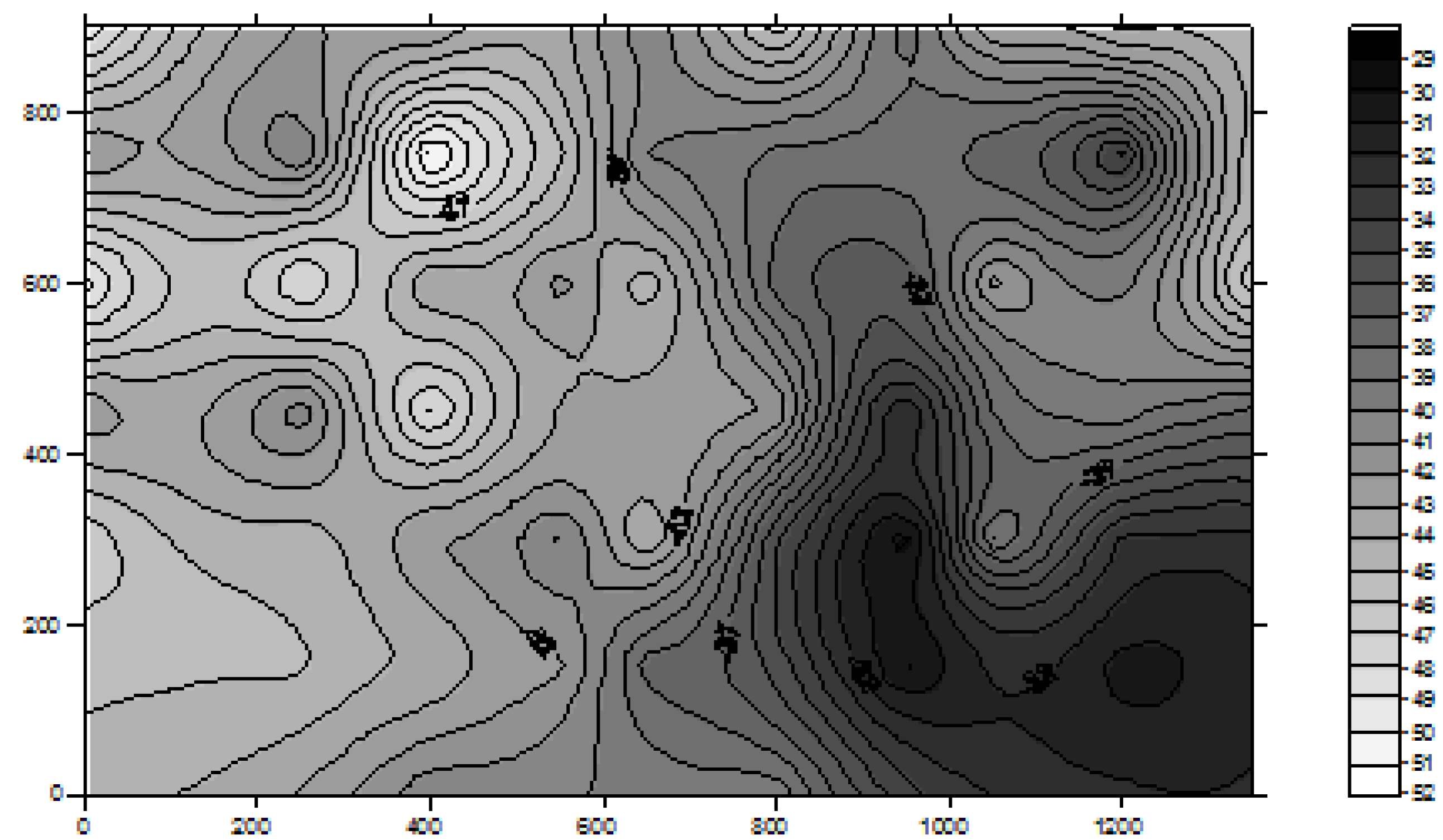
Figure 1.
An example of radio map generated from a Wi-Fi signal strength database.
Figure 1.
An example of radio map generated from a Wi-Fi signal strength database.
In real-time positioning, the RSSs collected at an unknown position are compared with radio map’s pattern. The pattern comparison algorithms can be generally classified into deterministic and statistical approaches which include point matching, area based probability and Bayesian network [7]. Recent research outputs on the statistical methods include but not limited to, for example, the Expectation–Maximization (EM) algorithm [8], Coverage Area Estimates [9], and floor determination algorithms for Wi-Fi positioning in multi-storey buildings proposed by [10,11].
In this paper, our proposed neural network algorithm is compared with the point matching approach based on the minimum norm principle as described below.
The minimum norm point matching method can be mathematically expressed as:
 where SSRM (i,j) is the RSS value of the signal transmitted from access point (i) at radio map point (j), and SSMEAS (i) is the measured RSS of the signal transmitted from access point (i). The radio map point (j) having the minimum norm is considered to be the most probable position. Since in the real-time positioning process the Wi-Fi sensor can be in any direction, a practical approach in the database development process is that, at each sampling point, the RSS data is firstly collected in a reference 0°, then 90°, 180°, and 270° directions, and the mean RSS value of the data collected in these four directions is used in the computation. It is obvious from Equation (1) that the positioning accuracy is dependent on the resolution of the calibration points, and the positioning results are always snapped to the discrete points’ position. Hence, the higher resolution the calibration points, the more accurate the result. However, as shown in Figure 1, the signal propagation from each available AP is a continuous non-linear surface. Therefore, a model that can best describe the surface of all APs’ signal propagation will help to improve the positioning accuracy. Due to the reflections of waves by obstacles and other interferences, the structure of the above functions could be rather complex. The traditional statistical methods based on some smoothing approximation may fail to capture the widely fluctuating characteristics of these wave patterns.
Since their emergence, the Neural Network of different types and structures has been used effectively in a number of cognitive processes. They have been shown to be able to detect some very subtle changes in observable data patterns. The activation (or transfer) functions that link one layer of neurons to the next are sigmoid instead of ordinary algebraic functions which render it highly responsive to any abrupt changes in the input data. In fact, it was proved by [12] that the Feed-forward Neural Networks with one input layer, one output layer and a single hidden layer with sigmoid activation functions are capable of approximating any Borel measurable function (that includes those functions described by the above patterns) to any desired degree of accuracy, provided sufficiently many hidden neuron units are available. Based on this finding, [13] introduced a 3-layer recurrent neural network with an efficient learning algorithm able to perform accurate currency exchange rates forecasting. In the following, the neural network modeling for the fingerprinting approach and experimental tests to validate the proposed algorithm are discussed.
2. Neural Network Modeling
From the above introduction of the fingerprinting positioning approach, it is possible to consider the co-ordinates ((x,y) in 2-dimensional case) of a point as a function of the signal strengths from several access points {si}, i = 1, 2, …, m, where, x = f(s1, s2, …, sm) and y = g(s1, s2, …, sm). If a sample of uniform (or random) distribution of points with known positions and the signal strengths from those access points can be measured accurately, the minimum norm as shown in Equation (1) or some well known statistical methods can sometimes give a fairly good approximation of the position of any other points in this region based on the measured signal strengths at this position. As explained in the previous section, the traditional statistical methods based on some smoothing approximation may fail to capture the widely fluctuating characteristics of these wave patterns produced by those access points. This explains the high errors in Wi-Fi positioning inside certain buildings [1].
With the above reason, a simple 3 layer Feed-forward Neural Network is considered to be an efficient learning algorithm for a more accurate position determination using Wi-Fi networks, and this Neural Network model is described below.
Let xi be the input of the average measured signal strength from access point i at the position P, where, i = 1, 2, …, m.
The output from neuron j in the hidden layer is given by
 where θj is the threshold parameter, and j = 1, 2, …, n, and the output coordinates (z1,z2) is given by
 where, φk is the threshold parameter.
Combining Equations (2) and (3), we have,
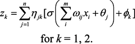
From Equation (4), we see that given a set of average weighted signal strengths from a set of m access points, with weights ωij ’s, the coordinates (z1, z2) correspond as the output from the network. Consider
 where βi,l are parameters to be included in our learning process with
 to give the best approximation.
The configuration of our proposed neural network is shown in Figure 2. It should be noted that the signal strength xi at a point P from access point i is initially taken to be the arithmetic mean of p (p = 3 or 4) signal levels measured at p appropriately chosen directions. Our learning process involves the determination of Parameters {ηjk}, {ωij}, {θj}, {ϕk} and {βi,l} so that the discrepancy output coordinates and the actual coordinates on a chosen set of points is minimal. More precisely; it is the actual coordinates (ẑ1, ẑ2) of a given point in our training set corresponding to the output (z1, z2); and the above parameters should be determined with the condition that the sum of squares of their difference is minimized. That is to minimize the expression
∑(z1 − ẑ1)2 + (z2 − ẑ2)2

Figure 2.
A three-layer feed-forward Neural Network for Wi-Fi positioning.
Figure 2.
A three-layer feed-forward Neural Network for Wi-Fi positioning.
Here the summation is taken over the entire training set. We shall see that the success of our learning process depends on whether we can get the smallest possible value for the above sum of squares of their difference or, in other words, the best learning surface that describes the actual RSS pattern generated by all the access points covering the whole region.
The minimization algorithm was adapted and modified from [14] that has been shown to be very efficient for solving a number of very difficult problems in least squares minimization. Since the objective function is nonlinear, a simple but effective heuristic optimization method introduced by [14] is used. It has been demonstrated to be efficient in a number of complex least squares minimization problems including the training of a recurrent neural network. The method contains three basic steps:
- (i)
- full local exploration
- (ii)
- partial local movement and
- (iii)
- exploratory movements
Each step is described briefly as follows.
(i) Full local exploration
Let x(k) be the kth approximation to the point where the minimum occurs and h be the step-length. The objective function at two sets of points about x(k) defined in Equations (8) and (9) is evaluated.
where ej = (0, …, 1, 0, …, 0) is the unit vector whose jth coordinate is one while the remaining coordinates are zero.
S1: x(k + 1) = x(k) ± hei
S2: x(k + 1) = x(k) ± hei ± hej
i = 1,2, …, n, j = 1,2, …, n, and j ≠ i
i = 1,2, …, n, j = 1,2, …, n, and j ≠ i
Consider that the first set of points lies uniformly on a sphere of radius h, while the second set S2 lies on a sphere of radius  h with the centre at x(k) obtained by taking the respective lengths of x(k+1) defined in Equations (8) and (9). This means that the total number of function evaluations is 2n(n − 1) + 2n = 2n2. It can be shown that the global minimum, if it exists, would most likely be entrapped lying inside this neighborhood.
h with the centre at x(k) obtained by taking the respective lengths of x(k+1) defined in Equations (8) and (9). This means that the total number of function evaluations is 2n(n − 1) + 2n = 2n2. It can be shown that the global minimum, if it exists, would most likely be entrapped lying inside this neighborhood.The search direction can be further refined as follows:
If f(x(k + 1)) ≤ f(x(k)) for some choices of i and j, then the function values at an additional set of 2(n − 1) points about x(k + 1) will be evaluated before performing partial local exploration in order to finely adjust search direction, that is, to set:
for some integer t values belonging to the set {1, 2, …, n} that gives the best function value.
x(k + 1) = x(k + 1) + het (or − het)
(ii) Partial Local Movement
This procedure helps us to decide when we should take a more aggressive move to reach the optimum from far away or when to take a more cautiously slow approach, when the true optimum is close by. The basic procedure is given in the following:
Let b = x(k+1) − x(k). We evaluate f at the following sets of points about x(k + 1):
for i = 1, 2, …, n, and εi = 1 or −1 according to the sign of the coordinates of b. Otherwise, set xs = x(k+1) ± b − hei and ei along the direction of b is excluded.
S1: xs = x(k + 1) + b
S2: xs = x(k + 1) + b − εihei
Now, if f(xs) ≤ f(x(k+1)) for some choice of i, then xs − x(k+1) definitely gives a better direction of descent and we can make exploratory moves, as described in (iii) below, along this direction. Otherwise, we have to reduce the step-length by D and start the full exploration again at x(k + 1). It should be noted that the order of iteration is linear with respect to n.
(iii) Exploratory Movement
The classical exploratory movement in “pattern search” heuristics or the corresponding “gradient method” can never be taken to full advantage if the path of displacement cannot be modified as the move proceeds. By properly adjusting the direction as the move proceeds from point to point, we can help guide our search much quicker to the true optimum. This could be done as follows:
Let m = xs − x(k), and evaluate f at the following points:
and ei along the direction of b is excluded.
S1: x(k + 2) = xs + m
S2: x(k + 2) = xs + m + hei
Notice that at most 2n + 1 function evaluations has to be performed.
(iv) Effect of Contraction Ratio and Initial Step Length
A contraction ratio of D = 4 can be seen to be the most appropriate choice. For, in the lower dimensional cases (i.e., the number of variables or parameters is not too large), if the true minimum happens to lie outside the reduced cube around the search position, it can be reached in a few steps. However, if the minimum happens to lie inside the reduced cube, the size of search space is significant comparing with that using contraction ratio of D = 2. The contraction ratio D = 3, though simple, would increase computer’s truncation error that would affect the computational accuracy. In the case where D = 4, the contracted length is one fourth of the original step size. If the minimum point happens to be x(k) again, one can be assured that the actual minimum point lies within these contracted spheres. Now, if the minimum value is at either one of the points on the contracted sphere S'1, (i.e., x(k + 1) = x(k) ± (h/4)ei for some i ) or one of the points on the contracted sphere S'2, (i.e., x(k + 1) = x(k) ± (h/4)ei ± (h/4)ej for some i and j), again only one full exploration around this point with step length h/4 will be needed to determine that the actual minimum probably lies within the contracted spheres; otherwise, one additional partial movement will lead the search outside this region. On the other hand, if the actual minimum point lies between the contracted outer sphere S'2 and the original outer sphere S2, it is easy to see that no more than four combined local or exploratory moves are required to reach it. In all cases, the order of complexity of search is n2, similar to those with lower contraction ratios. It was found by [14,15] that, for experimenting with most of the benchmark test examples, the best contraction ratios were D = 4, followed by D = 5. There was no gain in further increasing the contraction ratio, except in some rare cases.
(V) Termination Criteria
Terminate the search, if the step size is reduced to be less than a prescribed tolerance level. Care must be taken not to set the tolerance too low, otherwise, poorer results will be obtained even at the expense of longer computer time. In our learning process, we found from experimentation that the best tolerance is 1e−7.
The initial step-length affects the rate of convergence. In our test runs, the initial step-length of 0.25 gave satisfactory results in most of the benchmark test examples. Except in the cases where the objective function fluctuates wildly in part of the search region, a shorter step-length or a rescaling of the objective function might help in giving a more satisfactory convergence. Often, whether the initial step length is suitable or not, could be detected in the first few iterations.
To obtain the best learning result, the optimization process has to be rerun one or two more times with a new restarting point each time and select the best solution (i.e., the one that gives the least sum of square error). These restarting points can be chosen at random, but at a good distance from the previous starting positions or by following the procedure described in [15].
3. Algorithm Validation
The above algorithm was validated using data collected inside a building of the Hong Kong Polytechnic University (HKPolyU) campus, with the APs’ distribution shown in Figure 3.
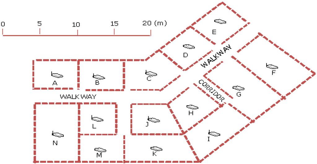
Figure 3.
Floor plan showing the distribution of access points in the test site.
Figure 3.
Floor plan showing the distribution of access points in the test site.

The 14 numbers of APs were labeled according to area number from A to N respectively. In our investigation, signal strength data from 3 and 4 numbers of APs were used for training by the neural network. As shown in Figure 4, each area contains about 4 to 5 training points separated between 3 and 4 m depending on the shape and size of the area. Data collected at other points, as an example shown in Figure 5 were then used to verify the accuracy achievement with the trained signal strength propagation surface. All locations shown in Figure 4, Figure 5 were able to receive AP signals from adjacent rooms as well as from other rooms within about 30 m radius. However, in our validation process, only signals from the nearest APs were used. As the IEEE 802.11 b/g standard Wi-Fi card was used for data collection, the signals received were at the same 2.4 GHz frequency.
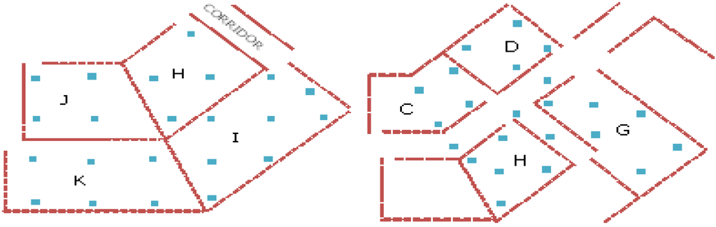
Figure 4.
An example of points selected for training by the neural network.
Figure 4.
An example of points selected for training by the neural network.
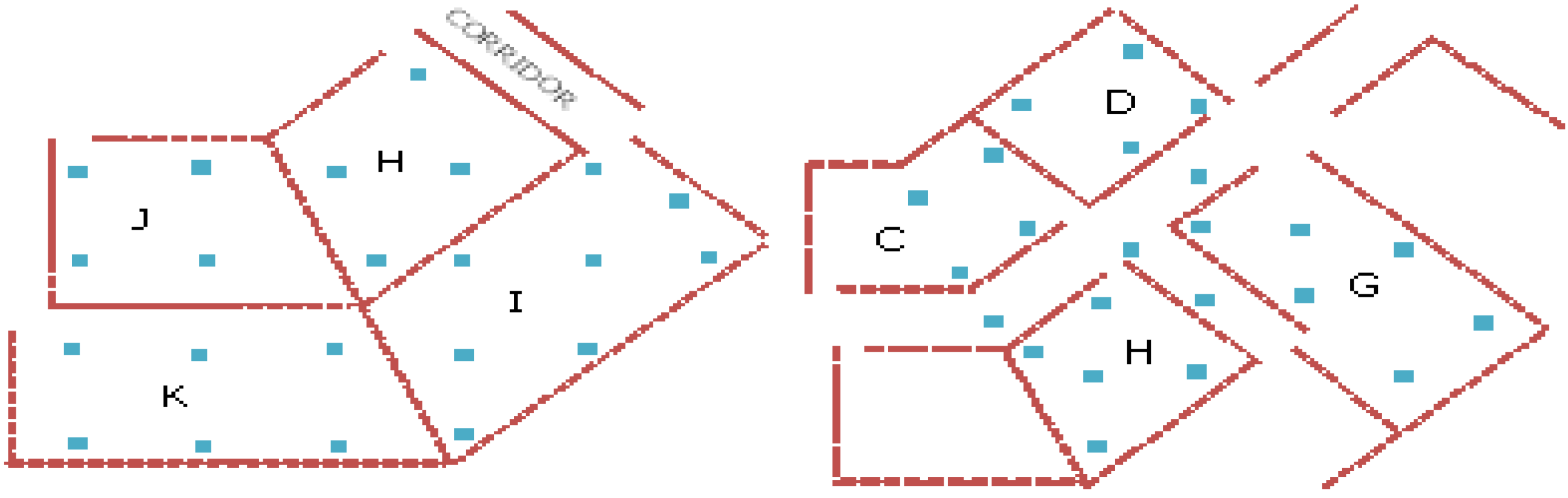
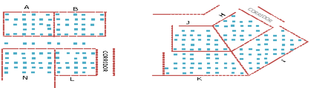
Figure 5.
Points with known position were used to verify the accuracy achievement of the neural network results.
Figure 5.
Points with known position were used to verify the accuracy achievement of the neural network results.
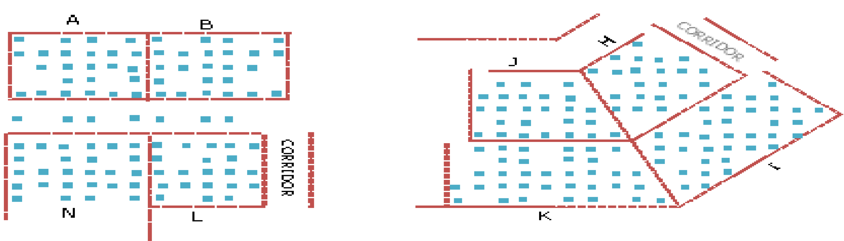
Table 1 shows the processed results using different combinations of four APs. For example, G_D_E_F represents the test verified with the data collected in rooms G, D, E and F with the RSS data transmitted from APs G, D, E and F (refer to Figure 3). The Table shows the success rate at different accuracy levels, the Mean Square Error (MSE) indicating the average minimization results in the neural network training process, and the total number of points used for verification. The MSE is computed by the formula  , where N represents the total number of points used for training.
, where N represents the total number of points used for training. 
Table 1.
Accuracy achievement based on signal reception of four access points (APs).
| 4-AP Combination | 0–1 m | 1.1–2 m | 2.1–3 m | 3.1–4 m | >4 m | 0–4 m | Mean Square Error | Total No. of Points |
|---|---|---|---|---|---|---|---|---|
| G_D_E_F | 3.5% | 14.1% | 28.2% | 15.3% | 38.8% | 61.2% | 5.5 | 85 |
| H_I_J_K | 0.9% | 7.8% | 12.1% | 15.5% | 63.8% | 36.2% | 26.7 | 116 |
| L_K_J_M | 7.7% | 24.0% | 32.7% | 14.4% | 21.2% | 78.8% | 10.8 | 104 |
| L_N_A_B | 9.8% | 24.5% | 26.5% | 13.7% | 25.5% | 74.5% | 2.6 | 102 |
| L_C_J_B | 1.8% | 8.3% | 14.7% | 20.2% | 55.0% | 45.0% | 23.2 | 109 |
| N_L_B_M | 18.1% | 28.7% | 20.2% | 9.6% | 23.4% | 76.6% | 2.7 | 94 |
| C_G_D_H | 14.0% | 23.3% | 22.1% | 10.5% | 30.2% | 69.8% | 8.7 | 86 |
| C_J_H_L | 1.3% | 8.8% | 8.8% | 15.0% | 66.3% | 33.8% | 5.1 | 80 |
| D_F_G_E | 1.1% | 7.7% | 24.2% | 22.0% | 45.1% | 54.9% | 13.6 | 91 |
| H_I_G_D | 2.9% | 10.8% | 13.7% | 19.6% | 52.9% | 47.1% | 12.3 | 102 |
Note: Initialization parameters used: βij = 0.25, ωij = 0.25, ηjk = 0.5, θj = 300, φk = 1.
Likewise, the processed results using different combinations of three APs are shown in Table 2. It should be noted that the results shown in Table 1, Table 2 are processed by only one set of generally accepted initialization parameters. It will be shown below that different assignments of signal strength input sequence and the initialization parameters will result in the change in the direction and the scale of the input vector, and hence will generate different trained surfaces for position estimation, and the MSE can be used to effectively verify which input vector assignment will be most likely to provide the best positioning solution.
Table 2.
Accuracy achievement based on signal reception of three APs.
| 3-AP Combination | 0–1 m | 1.1–2 m | 2.1–3 m | 3.1–4 m | >4 m | 0–4 m | Mean Square Error | Total No. of Points |
|---|---|---|---|---|---|---|---|---|
| G_E_F | 17.6% | 24.7% | 11.8% | 20.0% | 25.9% | 74.1% | 4.0 | 85 |
| H_I_K | 9.5% | 40.5% | 28.4% | 19.8% | 1.7% | 98.3% | 4.8 | 116 |
| K_J_M | 6.7% | 20.2% | 26.0% | 24.0% | 23.1% | 76.9% | 3.7 | 104 |
| L_N_B | 5.9% | 12.7% | 20.6% | 17.6% | 43.1% | 56.9% | 7.7 | 102 |
| C_J_B | 15.6% | 40.4% | 26.6% | 5.5% | 11.9% | 88.1% | 5.3 | 109 |
| N_L_M | 2.1% | 14.9% | 17.0% | 19.1% | 46.8% | 53.2% | 8.2 | 94 |
| G_D_H | 22.1% | 37.2% | 24.4% | 3.5% | 12.8% | 87.2% | 4.3 | 86 |
| C_J_H | 8.8% | 11.3% | 30.0% | 22.5% | 27.5% | 72.5% | 9.8 | 80 |
| D_G_E | 5.5% | 17.6% | 28.6% | 17.6% | 30.8% | 69.2% | 12.7 | 91 |
| H_I_G | 2.0% | 6.9% | 7.8% | 14.7% | 68.6% | 31.4% | 14.3 | 102 |
| H_I_J | 1.7% | 9.5% | 18.1% | 21.6% | 49.1% | 50.9% | 13.4 | 116 |
| I_J_K | 5.2% | 14.7% | 26.7% | 18.1% | 35.3% | 64.7% | 8.9 | 116 |
| H_J_K | 10.3% | 19.0% | 25.0% | 19.0% | 26.7% | 73.3% | 6.1 | 116 |
Note: Initialization parameters used : βij = 0.25, ωij = 0.25, ηjk = 0.5, θj = 300, φk = 1.
It can be seen from Table 1, Table 2 that different AP combinations would yield different accuracy achievement. It is understandable that the signal propagation paths are different, resulting in different signal interferences. Moreover, by inspecting the 0–4 m success rate and the MSE columns, an obvious trend can be found is that, the lower the MSE, the higher the achievement percentage. In order to further investigate this trend, all processed results were used to plot the graph of percentage of accuracy against MSE. It is clearly shown in Figure 6 that, in addition to the obvious negative correlation between the two components, most results with the MSE less than 5 would yield 80%–100% success rate. This initial analysis indicates that some of the results shown in Table 1, Table 2, particularly those with high MSE, were not determined based on the best fitted neural network trained surface. Nevertheless, to verify the validity of the algorithm, the data of 3-AP combinations with MSE less than 5 shown in Table 2 were extracted compare with the minimum point matching method, with the neural network’s training data used as calibration points stored in the radio map’s database. Since the radio map’s data are largely distributed in a 3 m grid, the point matching method would have the advantage of snapping the test points to the neighboring grid points, therefore the a high success rate of 2 m or better, and very high 4 m or better accuracy achievements are expected. The point matching results can hence form a good comparison base as the highest possible solution for verifying the effectiveness of the neural network algorithm. Their comparisons are summarized in Table 3.

Figure 6.
Relationship between mean square error and accuracy.
Figure 6.
Relationship between mean square error and accuracy.
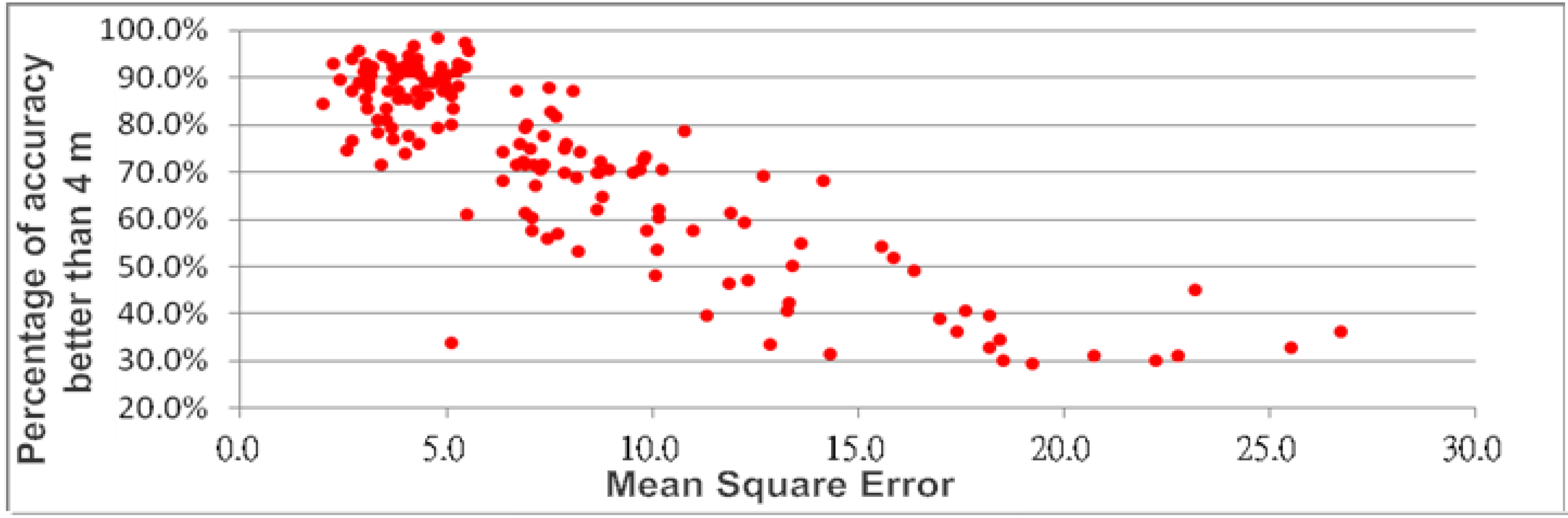
Table 3.
Comparison of accuracy achievement between the neural network and the minimum point matching methods.
| Neural Network | Point Matching | |||||
|---|---|---|---|---|---|---|
| 3-AP Combination | 0–2 m | 2.1–4 m | Mean Square Error | 0–2 m | 2.1–4 m | Total No. of Points |
| G_E_F | 42.3% | 31.8% | 4.0 | 47.1% | 31.8% | 85 |
| H_I_K | 50.0% | 48.2% | 4.8 | 59.5% | 29.3% | 116 |
| K_J_M | 26.9% | 50.0% | 3.7 | 63.4% | 25.9% | 104 |
| G_D_H | 59.3% | 27.9% | 4.3 | 58.1% | 30.2% | 86 |
It can be seen that the success rate of the two approaches are in general very similar except the K_J_M combination that, the 0–2 m accuracy for the point matching method is significantly better. It should be noted that only a set of constant initialization parameters was used in the neural network training process. This set of parameters may not produce the best trained surface for position determination. In fact, some of the solutions so obtained may just be local minima due to high complexity of our problem. Thus the actual implementation of the 3 steps proposed in Section 2 for generating the optimum RSS surface for Wi-Fi positioning need to be further investigated and verified. Observe that the 3-AP combination of I_J_K shown in Table 2 has the MSE of 8.9 and a low 0–4 m accuracy of 64.7%. This combination is used to illustrate our investigation.
The first investigation is the effect of the trained surface by varying the initial parameters. Parameters βij = 0.25, θj = 300 and φk = 1 were considered to be acceptable settings, they were fixed in our investigation in order to improve the training efficiency. Parameters ωij and ηjk were varied between the following ranges and increments,
- ωij = 0.10 to 0.50, step 0.05
- ηjk = 0.1 to 0.9, step 0.1
Table 4 shows the processed results of I_J_K using three different sets of initialization parameters. It can be seen that the second set of parameters yields the least MSE of 4.2 among the three, and the 4 m or better accuracy has been increased from 31.0% to 91.4%. Further compare the set 2 results with the point matching results, it can be seen in Table 5 that the overall success rate (4 m or better) of the neural network method is better than the point matching method.
Table 4.
Results of varied initialization parameters for the 3-AP I_J_K combination.
| Initialization Parameters | 0–1 m | 1.1–2 m | 2.1–3 m | 3.1–4 m | >4 m | 0–4 m | Mean Square Error | Total No. of Points |
|---|---|---|---|---|---|---|---|---|
| Set 1 | 8.6% | 19.8% | 26.7% | 20.7% | 24.1% | 75.9% | 7.9 | 116 |
| Set 2 | 12.9% | 34.5% | 37.1% | 6.9% | 8.6% | 91.4% | 4.2 | 116 |
| Set 3 | 2.6% | 8.6% | 7.8% | 12.1% | 69.0% | 31.0% | 22.7 | 116 |
- Set 1: βil = 0.25, ωij = 0.1, ηjk = 0.9, θj = 300, φk = 1;
- Set 2 : βil = 0.25, ωij = 0.5, ηjk = 0.1, θj = 300, φk = 1;
- Set 3 : βil = 0.25, ωij = 0.5, ηjk = 0.9, θj = 300, φk = 1.
Table 5.
Comparison of the neural network and the point matching method using the lowest MSE of the I_J_K combination.
| Accuracy | Point Matching | Neural Network |
|---|---|---|
| 0–2 m | 60.4% | 44.8% |
| 2.1–4 m | 26.7% | 46.5% |
| 0–4 m | 87.1% | 91.3% |
The second investigation is the variation of the input order of the signal strength from the three APs with a set of fixed parameter setting. A typical set of results is shown in Table 6. It can be seen that the variation of the APs’ input order would significantly change the MSE as well as the accuracy achievement. (Observe that the two input order sequences in the middle rows of the table reduce the mean square error by approximately 20%, while increase the proportion of 0–4 m accuracy by at least 4.5% relative to the remaining four settings).
Table 6.
Results of different order of three APs used for neural network training.
| Sequence of Combination | 0–1 m | 1.1–2 m | 2.1–3 m | 3.1–4 m | >4 m | 0–4 m | Mean Square Error |
|---|---|---|---|---|---|---|---|
| I_J_K | 8.5% | 19.1% | 24.0% | 18.1% | 30.4% | 69.6% | 8.7 |
| I_K_J | 8.1% | 20.2% | 24.4% | 17.1% | 30.2% | 69.8% | 8.2 |
| J_I_K | 11.4% | 24.6% | 26.6% | 15.8% | 21.6% | 78.4% | 6.4 |
| J_K_I | 11.3% | 24.7% | 25.8% | 16.7% | 21.4% | 78.6% | 6.4 |
| K_I_J | 9.0% | 20.9% | 24.6% | 19.2% | 26.3% | 73.7% | 8.1 |
| K_J_I | 9.9% | 22.0% | 24.6% | 17.4% | 26.1% | 73.9% | 7.8 |
The above tests and comparison studies have confirmed the effectiveness of our proposed algorithm. Based on our experience, the 3-step heuristic optimization method can be effectively implemented by varying parameters ωij (0.1 to 0.5) and ηjk (0.1 to 0.9), and changing the input order of the AP combination to obtain the best trained surface.
4. Conclusions
From our investigations, Wi-Fi positioning can generally achieve 1 to 4 m of accuracy in an arbitrary Wi-Fi network area using the neural network approach. However, the training process and parameter selection of the neural network is the key for achieving the highest possible accuracy of Wi-Fi positioning results. Our experimental results show that the proposed neural network improves the accuracy of positioning significantly by improving the nonlinear, highly complex Wi-Fi signal propagation patterns. To avoid being trapped in a local minimum, training should be permitted to retry with different initial parameter settings and different order of AP data inputs, so that the best set of parameters (i.e., the one that gives the lowest objective value) can be found. This will improve the overall accuracy. We have shown that there is a negative relationship between the mean square error value attained in our training process and the percentage of accuracy in our positioning. This means that based on the plot in Figure 6, one can repeat the training process as described above in order to achieve the highest possible accuracy.
The following summarizes the advantages of our proposed algorithm:
- This algorithm is based on the Wi-Fi fingerprinting approach that, Wi-Fi AP’s coordinates are not required in the position determination process. It is suitable for establishing a Wi-Fi based positioning system in areas such as inside shopping malls where APs’ positions are difficult or not possible to be precisely determined.
- This approach is entirely general and flexible. Whenever there are some changes in the existing Wi-Fi network (e.g., some addition, or deletion or reposition of access points), all we have to do is to retrain our neural network properly.
- There is no limit to how close our neural network approximation is to the actual radio data pattern (or hyper-surface), as long as we have sufficiently large number of neurons in the hidden layer of our simple three layer feed-forward neural network. However, it should be noted that, a too large number of neurons in the middle layer may render the learning process less tractable and higher truncation error. This is because the more complex structure of the function to be minimized may offset some of its improved accuracy.
- Since the percentage of better than four meter accuracy is found graphically to be inversely proportional to the mean square error in our training process, one can improve it to any desirable proportion by further minimizing. It has been illustrated that one can get closer to the actual minimum square error by retraining the neural network with different initial parameter settings, our optimization algorithm is simple and effective, and can be further improved or replaced by another even more powerful one with basically no change in our model structure.
In our investigation, only the minimum norm point matching method is compared with our proposed algorithm. As addressed in the Introduction section, many other effective Wi-Fi positioning algorithms have been proposed recently. It would be worthwhile to further investigate the strengths of each approach under different geometrical, access point availability and distribution, and influence conditions, for developing a reliable ubiquitous positioning system with the best achievable accuracy, to also support Global Satellite Navigation Systems (GNSS) in case satellite positioning fails in highly obstructed outdoor environments.
Acknowledgements
This research is fully supported by UGC Research Grant BQ-936 “Intelligent Geolocation Algorithms for Location-based Services”. The authors would like to thank Jeffrey Yiu for his assistance in the field tests and data processing of the investigations presented in this paper.
Conflict of Interest
The authors declare no conflict of interest.
References
- Mok, E.; Yuen, K.Y. A study on the use of Wi-Fi positioning technology for wayfinding in large shopping centers. Asian Geogr. 2013, 30, 55–64. [Google Scholar] [CrossRef]
- Mok, E.; Retscher, G. Location determination using WiFi fingerprinting versus WiFi trilateration. J. Location Based Serv. 2007, 1, 145–159. [Google Scholar] [CrossRef]
- Wang, J.; Urriza, P.; Han, Y.; Cabric, D. Weighted centroid algorithm for estimating primary user location: Theoretical analysis and distributed implementation. Trans. Wirel. Commun. 2011, 10, 3403–3413. [Google Scholar] [CrossRef]
- Theodore, S.R. Wireless Communications, Principles and Practice, 2nd ed.; Prentice-Hall, Inc.: Upper Saddle River, NJ, USA, 2002; p. 693. [Google Scholar]
- Cho, Y.; Ji, M.; Lee, Y.; Kim, J.; Park, S. Improved Wi-Fi AP Positioning Estimation Using Regression Based Approach. In Proceedings of the 3rd Proceedings of International Conference on Indoor Positioning and Indoor Navigation (IPIN), Sydney, Australia, 13–15 November 2012.
- Nurminen, H.; Talvitie, J.; Ali-Loytty, S.; Muller, P.; Lohan, E.; Piche, R.; Renfors, M. Statistical Path Loss Parameter Estimation and Positioning Using RSS Measurements in Indoor Wireless Networks. In Proceedings of the 3rd Proceedings of International Conference on Indoor Positioning and Indoor Navigation (IPIN), Sydney, Australia, 13–15 November 2012.
- Elnahrawy, E.; Li, X.; Martin, R.P. The Limits of Localization Using Signal Strength: A Comparative Study. In Proceedings of 2004 First Annual IEEE Communications Society Conference on Sensor and Ad Hoc Communications and Networks (IEEE SECON 2004), Santa Clara, CA, USA, 4–7 October 2004; pp. 406–414.
- Addesso, P.; Bruno, L.; Restaino, R. Adaptive Localization Techniques in WiFi Environments. In Proceedings of 5th IEEE International Symposium on Wireless Pervasive Computing, Modena, Italy, 5–7 May 2010; pp. 289–294.
- Koski, L.; PERÄLÄ, T.; PICHÉ, R. Indoor Positioning Using WLAN Coverage Area Estimates. In Proceedings of the 1st International Conference on Indoor Positioning and Indoor Navigation (IPIN), ETH Zurich, Zurich, Switzerland, 15–17 September 2010.
- Liu, H.H.; Yang, Y.N. WiFi-Based Indoor Positioning for Multi-Floor Environment. In Proceedings of the IEEE TENCON 2011, Bali, Indonesia, 21–24 November 2011; pp. 597–601.
- Shi, J.; Shin, Y. A Low-Complexity Floor Determination Method Based on WiFi for Multi-Floor Buildings. In Proceedings of the 9th Advanced International Conference on Telecommunications, Rome, Italy, 23–28 June 2013.
- Hornik, K.; Stinchcombe, H.; White, H. Multilayer feedforward networks are universal approximators. Neural Netw. 1989, 2, 359–366. [Google Scholar] [CrossRef]
- Li, L.K.; Cheung, B.K.-S. Learning and Forecasting Foreign Exchange Rates using Recurrent Neural Network Dynamics; Les Cahiers du GERADG-2000-02; GERAD: Montreal, QC, Canada.
- Cheung, B.K.-S.; Ng, A.C.L. An efficient and reliable algorithm for nonsmooth nonlinear optimization. Neural Parallel Sci. Comput. 1995, 3, 115–128. [Google Scholar]
- Cheung, B.K.-S.; Ng, A.C.L. An efficient search method for nonsmooth nonlinear optimization problems with mostly simple constraints. Neural Parallel Sci. Comput. 1997, 5, 335–346. [Google Scholar]
© 2013 by the authors; licensee MDPI, Basel, Switzerland. This article is an open access article distributed under the terms and conditions of the Creative Commons Attribution license (http://creativecommons.org/licenses/by/3.0/).