1. Introduction
Indoor localization is an ongoing field of research with new realizations of hardware, position estimation algorithms, calibration methods, and applications being developed every year. In the past decade, local positioning systems (LPS) based on ultrasound (US) have been established which are mostly intended for locating moving devices and persons. However, locating of numerous quasi-static devices integrated in a network is also important where US locating with high accuracy offers significant advantages for these systems. A wireless sensor network (WSN) with numerous nodes can be used as an example. Many applications dedicated to WSN can be significantly improved by node locating, e.g., network integration of nodes, supply node locations to application programs, supervising locations with respect to accidentally dislocating, detecting faking of node locations, and automatic device setup and security aspects in building networks [
1,
2]. Several design concepts for US locating systems have been presented. The concepts of these systems are influenced by a wide range of parameters, which will be briefly discussed in the following. For a more thorough discussion of this topic, the interested reader is referred to [
3] where the most important properties are summarized in this section.
In order to find device locations, systems perform time-of-flight (ToF) or time-difference-of-arrival (TDoA) measurements with well-known beacon positions. The benefit of using a TDoA system is that synchronization between the transmitting and receiving devices is not required thus reducing system costs by avoiding a second communication channel, e.g., by radio frequency transmission or using an infrared link. The ToF and TDoA measurements can then be related to distance and distance-difference measurements using the speed of sound which is 343.2 m/s in dry air at 20 °C (68 °F). Locations can then be obtained by tri- or multilateration for the ToF and TDoA case respectively. As the speed of sound changes with ~0.6 m/s/°C a LPS aiming for high accuracy needs some method for compensation of changes in the speed of sound, e.g., a temperature measurement or the use of a reference distance.
Another very basic design decision is whether the located device is transmitting an US signal and the beacons are receiving the signal or vice-versa. This is a crucial design decision when considering the locating of numerous devices. If the localized devices are actively transmitting US pulses, a media access protocol is required where code division multiple access method (CDMA) and time division multiple access method (TDMA) are the most common ones. On average scalability of such systems is rather limited. If the localized devices are passive and the beacons are transmitting, a single locating sequence allows locating of all devices in parallel. The locating rate depends only on how fast the sequence can be repeated where collision avoidance of the US signals again can be implemented by CDMA or TDMA. An advantage of passive locating is privacy of located devices which is sometimes claimed and which is given in a passive system because located devices do not emit any information which could be traced.
Common to all LPS systems is that the positions of the beacons have to be determined. This process is called calibration of the LPS and can either be performed manually by establishing a system of coordinates and measuring the beacon positions or by an automatic calibration algorithm. Final accuracy of an LPS is always a combination of the accuracy of the localization and the accuracy of the beacon positions. If a quantitative judgment on the accuracy of the system is desired care must be taken that the individual systematic and random components can be assessed individually.
2. Related Work
Two types of system configurations can be distinguished by the role of the mobile nodes. In an active LPS, the mobile nodes emit ultrasound (US) and the beacons are receivers. This is for example the case in BAT [
4], the pioneer of US LPS, and the recently developed SNoW Bat [
5]. On average, scalability of such systems is rather limited because the number of concurrently transmitted signals lowers the SNR. For example, [
6] reported that for more than 16 concurrent transmitters the bit error rate was already severely deteriorated and no longer allowed correct transmitter identification. If concurrent access is not (or no longer) possible, the locating rate starts to decay and is inversely proportional to the number of nodes. This has already been discussed in [
7] for the Active Bat system where complex workarounds are necessary increasing system complexity and cost. Contrary to the two previous systems, Cricket [
8,
9], the first BLUPS [
10] and other systems [
11] use transmitting beacons and receiving nodes. Reported position errors are less than 9 cm for BAT [
4], less than 1.5 cm for SNoW BAT [
5], 30 cm for Cricket V1 [
9], 1 cm for Cricket V2 [
9], and 1.5 cm for BLUPS [
10].
The time of flight (ToF) method for ranging measurement is used to deliver fine-grained localization in [
4,
5,
8,
9,
10]. A System using time differences of arrival (TDoA) is [
6]. Robustness to different failures in ToF/TDoA measurements is an important aspect as lightweight obstructions around the receiver will introduce bending and refracting effects and can introduce an error of up to 5% [
12]. Non Line of Sight (NLoS) errors with different size of object and position can be between 10% and 100% [
12]. It is also known that the traditional least squares multilateration algorithm delivers inaccurate results if there is a single error in measured distances [
13]. For example [
12] used the least median of squares (LMedS) which delivers improved performance in case of NLOS signals.
For achieving high accuracy in a LPS, calibration is of upmost importance because the correct position of beacons will directly influence the accuracy. This is obvious because these positions are used in the formulas for multilateration. Different calibration methods have been proposed: In [
14], the ceiling mounted receivers were calibrated by a transmitter moving to at least five known coordinate points. DOLPHIN [
15] is a distributed positioning system aimed at ubiquitous computing applications. It applies iterative multilateration techniques where three precise positions of devices have to be defined as initial state. An auto calibration algorithm also requiring three known tests points for the ToF and TDoA case is presented in [
11]. Different types of measuring devices as required by [
11,
14,
15] can be used depending on the budget available. If low cost devices are used, e.g., simple measurement tapes, this will almost always reduce the final location accuracy. A lightweight 3D tag system using a calibration device is shown in [
16] where the average error was between 19.5 cm and 23.9 cm depending on the method used.
An auto calibration algorithm requiring no additional devices developed for LPS [
17] is based on multidimensional nonlinear least squares fitting algorithm. In [
18] a two-step self-calibration method is proposed which does not require any pre-calibrated positions if relative positions are sufficient. In order to perform that task no additional hardware besides US receivers or transmitters and radio transceivers, which are already available for a WSN, are required. It achieved very good position accuracy in the range of millimeter by simulation.
Verification of the calibration by comparing with manual calibration as in [
11] is not recommend because of the inability to establish an orthogonal coordinate system. The only quantity, which can be easily verified, is a point-to-point distance but not the individual coordinates due to the lack of the coordinate system unity vectors. Remarkably, an average deviation of only 2.2 cm has been achieved in [
11].
This article describes the LPS
LOSNUS (Localization of Sensor Nodes by Ultra Sound) [
3] as a complete and independent LPS where the same system can be used for calibration and localization. It enables a calibration process without expensive tools and/or laborious time in order to get accurate positions of beacons.
LOSNUS delivers high locating accuracy and can also tolerate single failures for the ToA measurements allowing arbitrary failure mode. Low cost and high accuracy are important properties of this system.
3. LOSNUS
3.1. Design Rationale of LOSNUS
Before explaining the individual components of the LPS LOSNUS, the design rationale is presented. As LOSNUS is designed for locating numerous mainly static nodes, the located devices are chosen as passive nodes and the beacons are active for best scalability. TDoA measurements have been chosen instead of ToF to avoid the necessity of a trigger signal between transmitter and receivers which otherwise would increase receiver complexity and costs. Accurate measurement of device positions is important if devices are nearby especially in case of measuring the same quantity (array). Therefore using broadband signals allowing the use of pulse compression techniques is a logical choice. Such techniques demand increased effort on the signal processing side at the receiver and therefore their complexity and number should be kept low. For this reason LOSNUS uses only a single linear frequency modulated chirp marking the signal arrival time with a following transmitter code. To avoid problems in case of signals transmitted in parallel LOSNUS uses a sequence of transmitting beacons, which avoids overlapping of line-of-sight (LOS) signals, but nevertheless delivers a medium fast locating rate. As non-line-of-sight (NLOS) signals are typically weaker than the LOS signals, a good SNR is obtained most of the times. Transmitters are identified using fixed frequency transmitter coding fields. An additional benefit is gained by non-parallel sending as the same amplifier can be used for all transmitting beacons if a low-cost demultiplexer is used. This is especially important in case of transducers requiring high driving voltage and/or large bandwidths, as these amplifiers are quite costly. Further cost reduction is possible by using 1-bit binary correlation at the receivers allowing the use of the synchronous serial interfaces present on modern microcontrollers for signal sampling. A receiver can therefore be realized by a low cost miniature ultrasonic MEMS microphone, a small preamplifier, a bandpass filter, and a 1-bit comparator interfacing to the microcontroller. An extension for low power applications is an optional starting sequence allowing wakeup of the microcontroller when a locating sequence is started. Memory requirements and computational complexity on the receiver can be reduced further by using a short lead-in for each LOSNUS frame time stamping the reception and starting the sampling of the LOSNUS frame. Expected system construction costs at volume quantities are below 5 USD for the receivers.
Calibration of LOSNUS can be performed directly with the installed beacons and a special receiver arrangement. For achieving high accuracy of beacon localization, the used receivers are synchronized with the transmission sequence, which can be realized with a wired link. This modification allows for measuring ToFs in order to achieve better convergence of the calibration algorithm. As calibration is a one-time process and stays valid unless transmitters are moved, this is the most economical solution. Further verification of the calibration of course can be performed in the TDoA system as well.
3.2. Basic Principle of LOSNUS
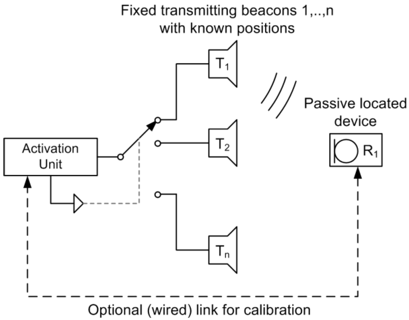
The basic system construction is shown in
Figure 1. Multiple active transmitting beacons are fixed at well-defined room positions.
Figure 1.
Basic localization of sensor nodes by Ultra Sound (LOSNUS) system architecture.
Figure 1.
Basic localization of sensor nodes by Ultra Sound (LOSNUS) system architecture.
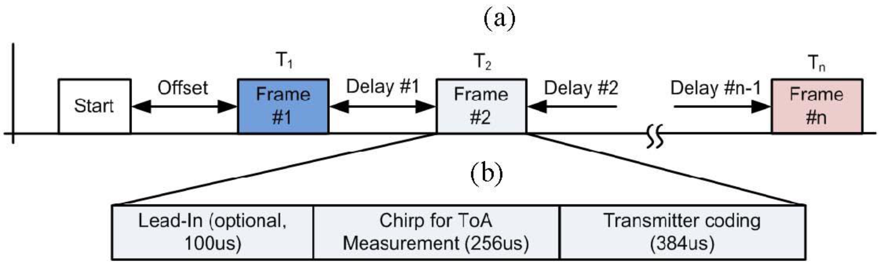
The locating process of
LOSNUS is started by a well-defined sequence of US signal frames shown in
Figure 2a. An activation unit sequentially activates each transmitter and emits at frame consisting of an optional lead-in, a linear frequency modulated chirp and a transmitter coding field shown in
Figure 2b. An optional starting sequence can be used for low power systems allowing remote wakeup of receiver units. Transmitting delays are chosen such that LOS signals of consecutive transmitters do not overlap at the receivers. In case of over-lapping of LOS and NLOS signals, perfect decoding of the larger LOS signal is common [
19]. Binary cross-correlation [
20,
21] of the received frame with the reference signal delivers high resolution ToA measurements. Once the start of the frame is known, the transmitter coding field can be easily analyzed. Transmitters are encoded using a fixed-frequency coding scheme where the number of transmitters is scalable by the number of frequency hops and slots used. Therefore, the concept is comparable to an N-FSK. Both signal processing and transmitter identifications are explained in more detail in
Section 3.3 and
Section 3.4.
The process described above delivers numerous pairs of ToA and transmitter IDs where always the first pair is selected corresponding to the LoS signal. The coordinate positions are then calculated using multilateration.
Figure 2.
Locating operation: Transmitting sequence (a), Transmitted frames (b).
Figure 2.
Locating operation: Transmitting sequence (a), Transmitted frames (b).
3.3. Signal Processing
Signal processing for ToF or ToA systems is a compromise along three factors—range, resolution and repetition rate. For resolution, two aspects are important: The first is separation of two nearby targets, which are limited by ΔR ≤ c/(2B) where c is the speed of wave propagation and
B is the bandwidth [
22]. The second aspect is uncertainty of the ToF or ToA estimates where various techniques are available including different type of estimators like classical cross correlation (CC), generalized cross correlation (GCC), maximum likelihood (ML), least mean square adaptive filters (LMS) and others [
23]. Furthermore, the sample rate of the system, if low, can require the use of interpolation methods. Simple algorithms include parabolic interpolation of the correlation functions where more complex ones use different types of transforms or up-sampling methods [
24].
LOSNUS uses a linear frequency modulated chirp with binary cross correlation at a high sample rate.
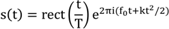
A linear frequency modulated chirp can be written as the real signal of the analytical waveform according to Equation (1) where T is the duration of the signal. The function rect is defined identical as in [
22] and is zero if |t| ≥ T/2 and 1 otherwise. The total frequency sweep is kT = Δ.
A very important property for a chirp is the dispersion factor or processing gain D = TΔ. The processing gain is the gain in the peak of the autocorrelation function for a pulse with equal range resolution. Furthermore it can be shown that for larger values of D the spectral amplitude of the chirp signal is approximately a rectangular window of width Δ. However, even for values of D as low as 10 about 95% of the energy are contained in the band Δ [
22].
Binary correlation for a discrete input signal r[n] with 0 ≤ n ≤ N and a reference signal s[m] with 0 ≤ m ≤ M − 1 is calculated according to Equation (2). Both input signals can have values of +1 and −1 respectively. The number of computations required is N·M. As both signals are binary, efficient and fast implementation is possible.
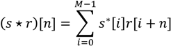
The most important properties for a linear chirp with the settings used in
LOSNUS are shown in
Figure 3a,b.
Figure 3a shows the theoretical 1-bit quantized chirp and
Figure 3b its binary waveform and autocorrelation function.
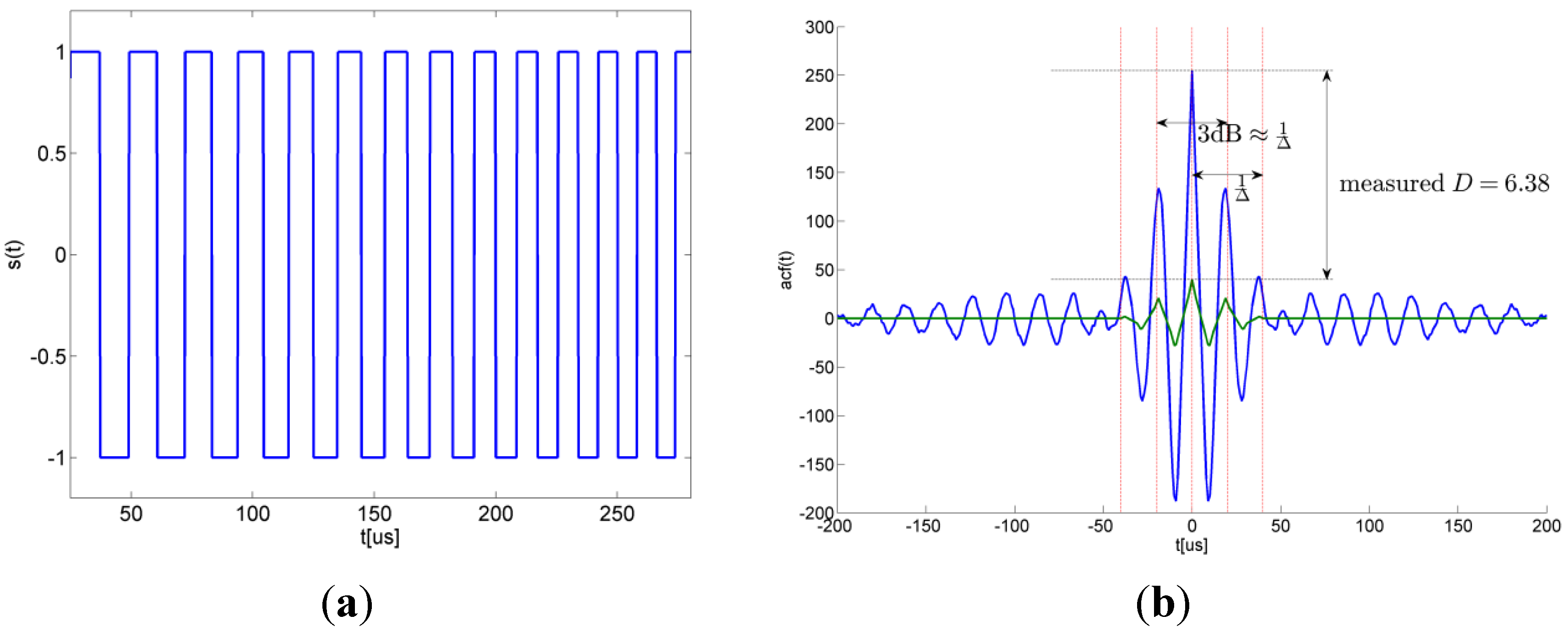
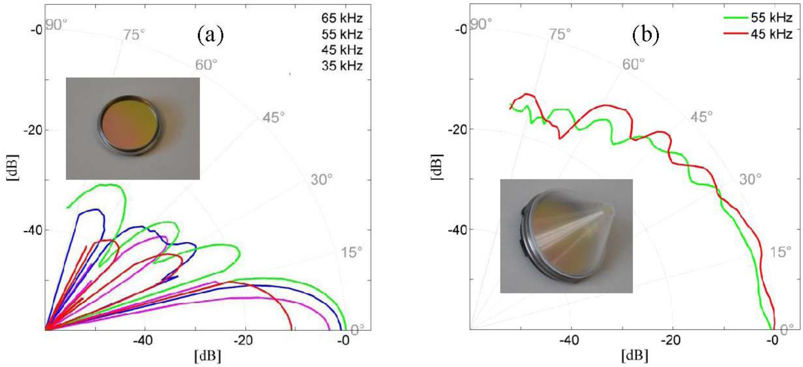
LOSNUS in this setup uses broadband electrostatic transducers from Senscomp allowing the transmission of such signals. One problem faced during system design was the coverage area as the broadband transducers have a frequency dependent radiation pattern. Signals resulting from directions outside the mainlobe are heavily changed in phase/amplitude and correlation can drop by more than 50% [
25]. For this reason a small cone has been attached to the sensors similar to [
26]. The resulting directivity diagrams before and after the modification are shown in
Figure 4a,b.
Figure 3.
(a) 1-bit quantized linear frequency modulated chirp with Δ = 25 kHz, f0 = 52.5 kHz and T = 256 μs; (b) Binary autocorrelation function (Theoretical D = 6.4).
Figure 3.
(a) 1-bit quantized linear frequency modulated chirp with Δ = 25 kHz, f0 = 52.5 kHz and T = 256 μs; (b) Binary autocorrelation function (Theoretical D = 6.4).
Figure 4.
(a) Directivity diagram without attached cone of Senscomp 600 electrostatic transducer; (b) Directivity diagram after application of cone.
Figure 4.
(a) Directivity diagram without attached cone of Senscomp 600 electrostatic transducer; (b) Directivity diagram after application of cone.
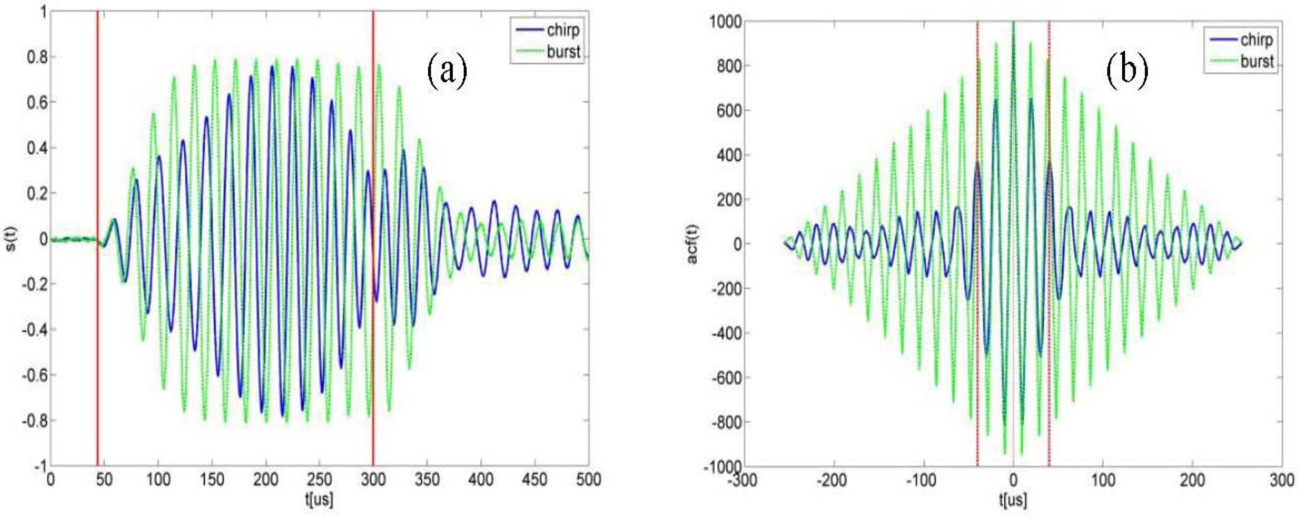
With the cone attached the waveform show in
Figure 5a was recorded using the linear frequency modulated chirp from
Figure 3a with driving amplitude of 160 Vpp and a DC Bias of 100 V. Using the signal of
Figure 5a in its 1-bit binary quantized representation its autocorrelation is shown in
Figure 5b. Results are still satisfying and the performance gain compared to a burst is easily seen. For comparison, in
Figure 5 the burst had equal length to the chirp as a small pulse is more difficult to measure. As the signal length is only 256 μs and the sample rate is 5 MS FFT, frequency resolution is low and the spectrum of the waveforms in
Figure 5a is not shown.
Figure 5.
(
a) Received (analog) waveforms for burst with f
0 = 52.5 kHz and chirp with settings from
Figure 3; (
b) Binary autocorrelation function showing pulse compression properties of the chirp compared to a burst.
Figure 5.
(
a) Received (analog) waveforms for burst with f
0 = 52.5 kHz and chirp with settings from
Figure 3; (
b) Binary autocorrelation function showing pulse compression properties of the chirp compared to a burst.
3.4. Transmitter Identification
Transmitter coding is realized as a fixed frequency coding with multiple time slots. As the starting time of the signal is known due to pulse compression of the preceding chirp, coherent N-FSK demodulation can be performed. Again, computational complexity is low because identification only needs to be performed on detected echoes and the signals are again 1-bit quantized. Furthermore processing can be performed on offline data if received frames are stored either on detection of a correlation peak or by the lead-in signal. For example, in the test setup with a total frame length of 740 µs (100 µs lead-in, 256 µs chirp and 384 µs transmitter encoding), storage requirements for a single frame are 740 Bit or 93 Byte. In case of six transmitters and assuming up to 5 NLOS echoes for each signal total storage requirements are 2.79 kByte. This is reasonable even on very low cost microcontrollers.
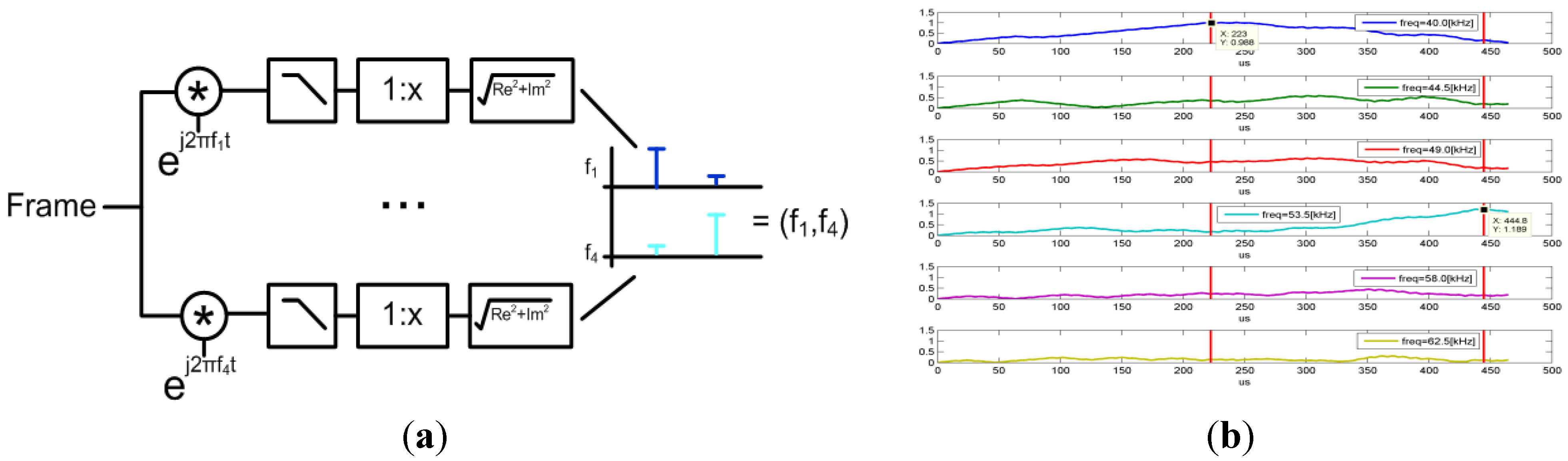
The basic decoding structure is shown in
Figure 6a. The binary input signal is multiplied by the different frequencies and low-pass filtered. The minimum length required by the filter in case of coherent demodulation is 1 divided by the frequency spacing. Knowing the starting time of the frame it suffices to evaluate the filter output at discrete multiplies of the symbol length. An example from a real measurement where six coding frequencies and two symbols have been used is shown in
Figure 6b. This already allows up to 36 transmitters sufficient for covering large rooms.
The computational complexity again is low and it requires for a sequence of length M and n transmitter coding frequencies n · M multiplications and additions at most. As the input sequence again is binary with values between +1 and −1 multiplication reduces to either a positive or negative summation.
Figure 6.
(a) Transmitter identification for n coding frequencies. Filter output values are only evaluated at discrete times as the starting time of the frame is known. (b) Example transmitter decoding on binary input data using fi = 40 kHz + 4.5 kHz · i, 0 ≤ i ≤ 5. Identified transmitter is (40 kHz, 53.5 kHz). Red vertical lines mark sampling points.
3.5. Localization
The LOSNUS localization algorithm is based on TDoA and requires the calibrated transmitter positions, the time differences and the speed of sound as an input. For two transmitters Ti and Tj, a receiver R and ToAs ti and tj the basic TDoA equation is given in Equation (3) where c is the speed of sound.
Having three such equations corresponding to four ToA measurements an analytical solution exists. An important parameter for a localization system is the dilution of precision (DOP) [
27], which relates ToA uncertainty to locating uncertainty. For example if the DOP is 20, the standard deviation of ToA measurements is 700 ns, and the speed of sound is 343 m/s then the standard deviation of the position estimate is 20 · 700 ns · 343 m/s = 4.8 mm. The DOP is dependent on the placement of the beacons and the position of the receiver.
As in a typical
LOSNUS system, more than four transmitters are available the redundancy in the data can be used for increasing the robustness of the locating procedure. The algorithm used by
LOSNUS is called
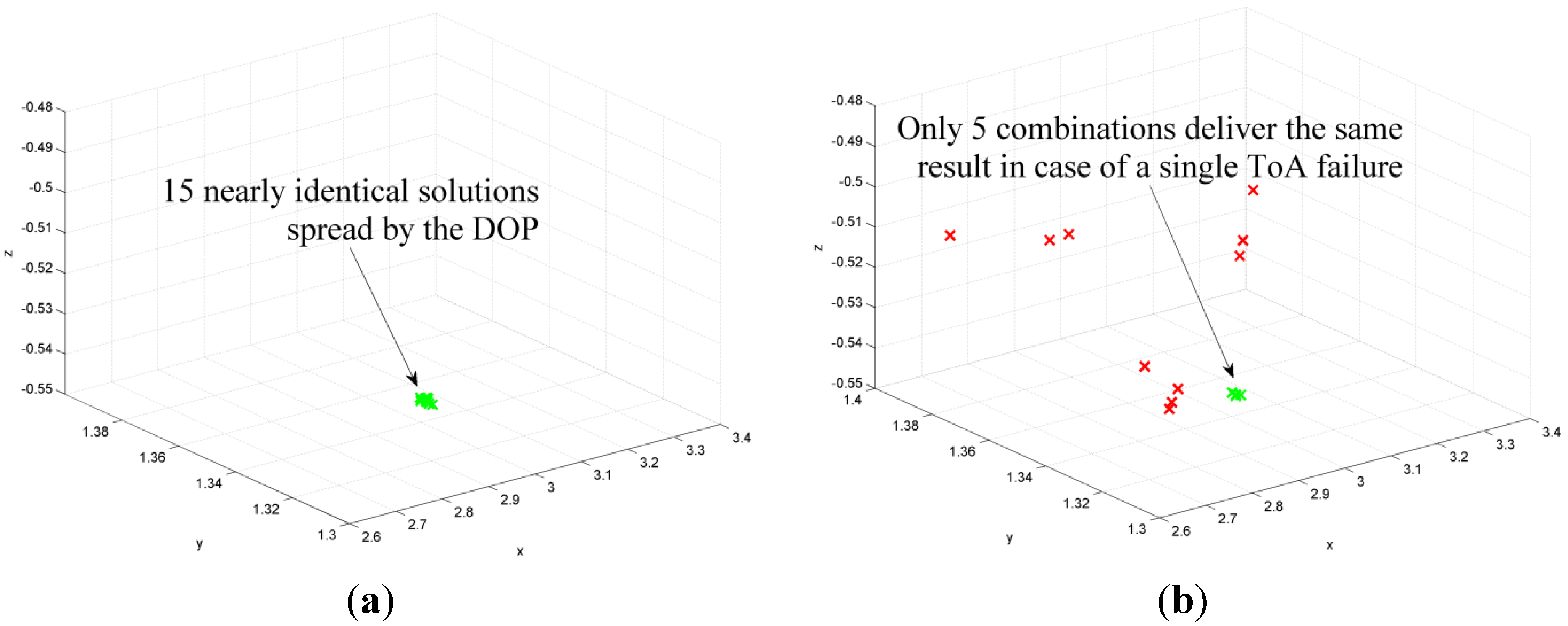
Grouping. Having six (or more) transmitters and requiring four ToAs for localization fifteen different combinations are possible. If all ToA combinations are valid then all calculated positions should be approximately the same. If one of them is incorrect, only five over four possible combinations are approximately the same, and the remaining ten positions are different.
Figure 7a shows that all fifteen solutions are close if no single ToA is an outlier.
Figure 7b shows the solutions when a single ToA was changed by 1 cm. It can be seen that the positions calculated by the correct combinations,
i.e., four over five, are still correct while all others a different.
In this situation, neither the non-linear least squares, nor using the mean or median of all coordinates can deliver the correct result. The algorithm creates distinctive groups whereas the elements are determined by a similarity scale based on calculating the 2-norm of all positions differences. The group with the largest cardinality is selected. The final position is either calculated by taking the mean of all positions within this group, by selecting the element with the lowest dilution of precision (DOP) for the transmitter/receiver combination or by applying an NLS algorithm to the correct ToAs. A comparison on the performance of the different position calculation methods as well as a comparison to other robust position estimation algorithms like Least-Median of Squared (LMedS) and Robust Multilateration (RMult) is shown in [
28]. Among the grouping algorithms, NLS performs best although the statistical differences are in the mm range. An important, but unproven aspect is that this algorithm requires that combinations including the wrong ToA do not form groups larger than the correct group. Simulation and practical results have shown us that this is indeed the case.
Figure 7.
(a) Calculation of the receiver positions by all fifteen combinations in case of no error. All positions are close and spread by the DOP. (b) In case of a single outlier only five combinations are still valid and all others deliver different results. The assumed ToA error for this example was 1 cm.
4. Calibration
Calibration of a LPS is essential before the system can be used to localize static nodes or mobile devices. Contrary to localization the LOSNUS calibration uses ToF and requires at least four receivers, six transmitters and a known reference distance in the currently used form. Using ToF was required because otherwise convergence of the calibration algorithm was not satisfying.
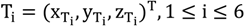
Calibration is performed by using six transmitters and four receivers where six out of the 30 coordinates are used for defining the coordinate system. Using the ToF and the speed of sound 24 equations can be found. Using proper minimization algorithms, the 24 unknown coordinates can be obtained. Let
![Ijgi 02 00908 i033]()
be the transmitters,
![Ijgi 02 00908 i034]()
, c the speed of sound and t
ij be the ToF between transmitter i and receiver j. The defining equations are then given by
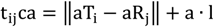
Due to the application of the cones for broadening the main lobe, the acoustic wave no longer directly propagates between the transmitter and receiver but first propagates from the transmitter to the opening of the cone. From there, it propagates to the receiver. Therefore, the previous equation has to be modified as shown in Equation (5) where the length of the acoustical cone is 1.
It can be shown that if a minimization algorithm solves equation system Equation (5) it also solves a scaled version of the system by a factor a, i.e., a geometrical expansion or compression.
This is an important result because no matter which speed of sound has been used the result of a calibration process is a scaled version of the physical system with the following consequence: Let r be a reference distance between to arbitrary receiver position. Then a post scaling factor can be calculated as
We therefore have exchanged the problem of knowing the accurate temperature to the problem of knowing a reference distance. Note that there has been placed no restriction on the type of reference distance which makes realization very easy. In this system, the reference path has been realized by using a mounted receiver on a linear belt and fixing two positions. The uncertainty of the belt was assumed to be 50 μm as manufacture data was not complete.
The calibration algorithm can be summarized as following: Based on guesses of the speed of sound, receiver and transmitters positions, a minimization algorithm is executed delivering positions T
i′, R
i′ and a cone length l′. As the speed of sound was only relatively correct but not absolutely the output is a scaled version of the system. By calculation of the factor a according to Equation (7) the final calibrated transmitter and receiver positions as well as the cone length are given by
Another important result is that a calibration performed with this approach is dependent on the accuracy of the reference path. The uncertainty of a transmitter (or receiver) can be estimated as:
For suppressing random components of ToF measurements averaging is necessary. The problem with averaging over a longer time is that an assumption of constant measurement conditions, especially temperature, is not realistic. This problem can be circumvented by assuming that the mechanical system is stable and the physical distances stay the same during the calibration process. As speed of sound is a scaling factor of the ToFs, the ratios have to remain the same. Multiple measurements ti(k) are performed where the scaling factor c(k) is defined by the sum of the 24 ToFs where the first measurement is arbitrarily used as reference.
Applying such a correction to each measurement retains the ratios but compensates the temperature. Using all of these techniques described above results in a high quality calibration and suitability of the approach was verified by simulations and a practical experiment.
5. Uncertainty
5.1. General Considerations
The accuracy of locating is based on two factors: accuracy of the system calibration and accuracy of the actual locating procedure. These two factors are completely independent being two different procedures performed at different points of time. System calibration is an operation done only once after system installation. Further on, the realized calibration accuracy is influencing any result of locating as the actual locating accuracy is an additional factor which reduces the overall accuracy.
Literature dealing with GPS and LPS is often defining its own meaning of the terms “accuracy” and “precision”, e.g., [
29]. In these definitions, accuracy is a combination of systematic and random components whereas precision is based on a confidence interval. This has multiple drawbacks, as one cannot individually differentiate between random and systematic components. In addition, the definition of accuracy carries a value of zero when accuracy is infinitely high. In this meaning these values represent deviations of real values.
The Guide (“Evaluation of measurement data—guide to the expression of uncertainty in measurement”) [
30], which is defined for generic use in measurements and is based on the term “uncertainty”, which is an interval set up around the measurement result containing the value of the measured quantity. “High accuracy”, which has only qualitative meaning and does not represent any value, is expressed by an uncertainty with low interval length. The term “precision” is not defined in GUM but in most cases the terms “random component of a measurement”, “repeatability” or “reproducibility” are a better choice. The GUM definitions are used in this article.
5.2. Uncertainty in ToF and TDoA Measurements
Using binary cross correlation for ToA/ToF measurements with the chirp settings of
Figure 3, the random component was tested to be normal distributed with a standard deviation of 400 ns or converted with the speed of sound at room temperature about 140 μm. The random component is a complex function of the electronics noise, microphone self-noise, acoustic noise (Brownian motion), sampling rate, length and bandwidth of the used chirp, which shall all be subsumed in above measure.
ToF and ToA measurements are modeled according to Equation (11) where in case of ToA the term t0 described the unknown transmission time. In the case of ToF, the term t0 contains any electrical and acoustic delays.
Time difference measurements are obtained by using one ToA as a reference. As measurements are uncorrelated the variances add.
Assuming a homogenous temperature, distances, pseudo-distances and distance differences can be calculated by scaling the ToF, ToA or TDoA measurements by the speed of sound. The temperature in this case is modeled assuming a systematic and a random component.
5.3. Uncertainty in Calibration
Using the proposed model for calibration, which includes ToF measurements (random and a systematic component), the acoustical delay of the cones (systematic component), a reference path with known uncertainty and a homogenous temperature within the room (systematic and random component), the obtained uncertainty for each calibrated transmitter position is:
T
i is the coordinate of the transmitter, u
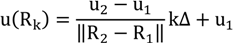
r is the uncertainty of the reference path and r is the length of the reference path. The same applies for the receivers R
i. All other systematic or random components are reduced either by the algorithms or averaging. A receiver-position used within the calibration is called reference position. Having two such positions available and a linear belt allows us to create arbitrary reference positions with a known uncertainty.
5.4. Uncertainty in Localization
For reporting the locating uncertainty, the concept F.2.4.5 of the GUM [
30] is applied. In this case, a known correction factor
b for a systematic effect is not applied but reported in the uncertainty of the measurement. Measurements are reported according to Equation (14) as three dimensional coordinates (x, y, z) including a systematic effect with unknown direction and a combined standard uncertainty also with unknown direction. P is the (unknown) value of the measurand. One should note that Equation (14) cannot be evaluated but is just a formal method for reporting results and should be interpreted as described herein.
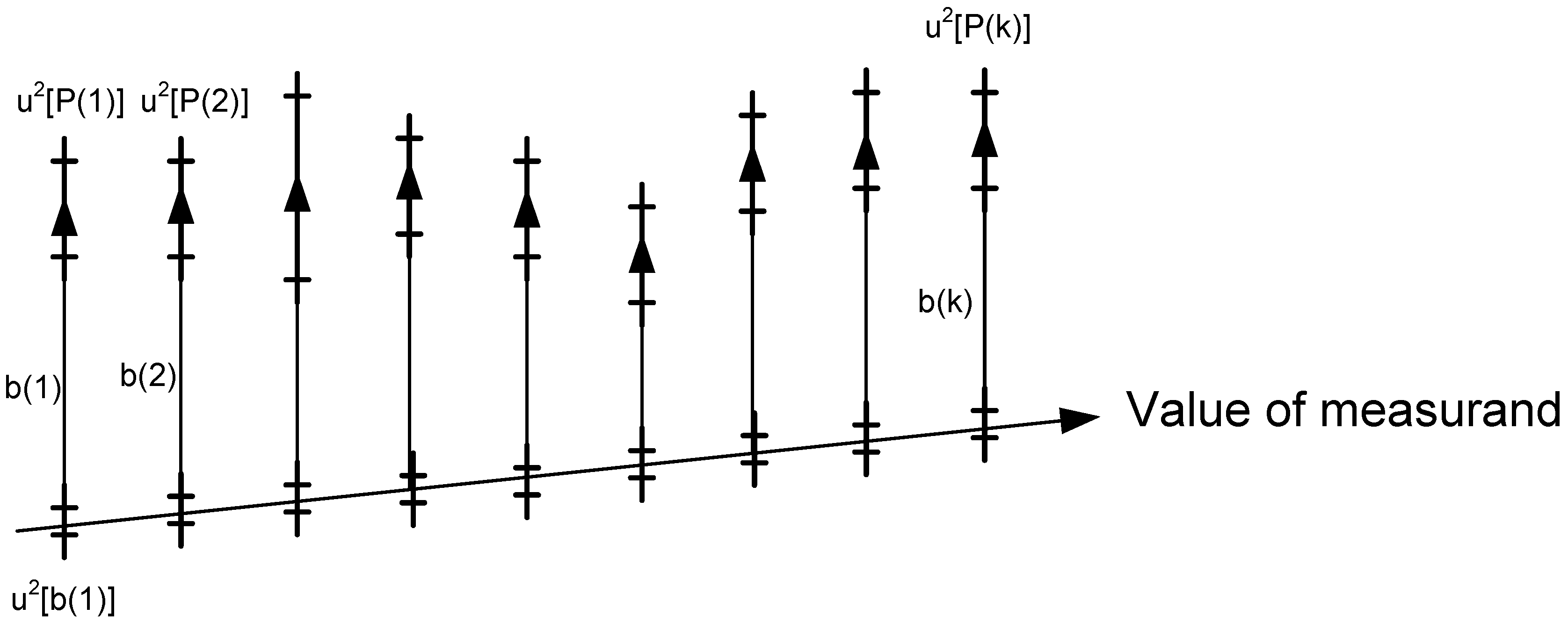
Figure 8.
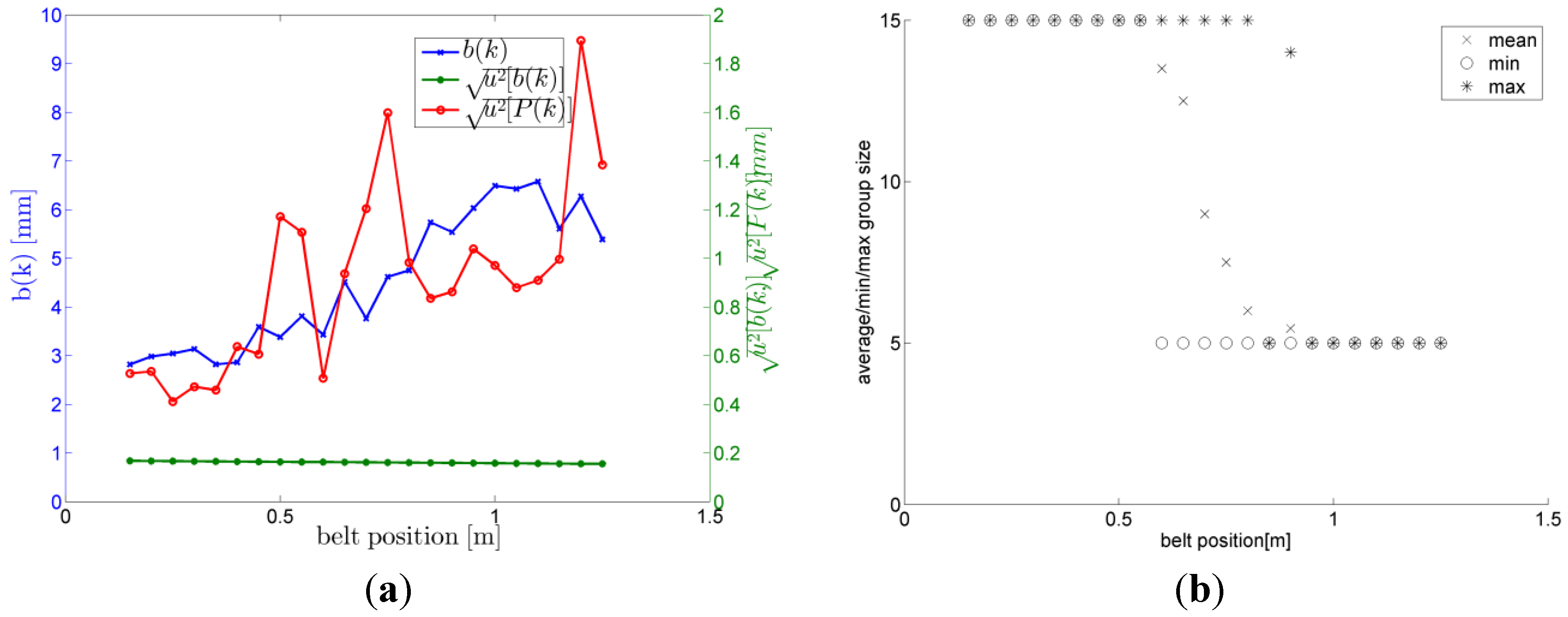
Graphical example for the calculation of uncertainty showing unknown value at the bottom, a systematic difference b(k) at each position, the uncertainty in determining b(k) as interval u2[b(k)] on the line tracking the value and the uncertainty of the individual measurements u2[P(k)].
Figure 8.
Graphical example for the calculation of uncertainty showing unknown value at the bottom, a systematic difference b(k) at each position, the uncertainty in determining b(k) as interval u2[b(k)] on the line tracking the value and the uncertainty of the individual measurements u2[P(k)].
The reported combined standard uncertainty u
c is defined as the positive square root of Equation (15). This complicated expression is explained in
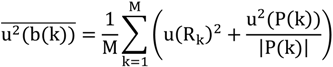
Figure 8. The index k identifies the position on the belt (23 positions in our case) whereas P(k) defines a sufficient set of measurements at this position (20 in our case).
The term u2[P(k)] is simply the variance for the measurements mainly resulting from the uncertainty of the TDoA measurements and the DOP. At each position, a systematic correction factor b(k) can be determined being the mean distance of the measurements to the interpolated reference position. As the value is not known the uncertainty for determining this factor is expressed by u2[b(k)] resulting from the inaccurate reference positions and the variance of the mean value of the measurements. As only a single systematic value b is determined u2[b(k)] describes the variance of the factor itself. An important aspect of applying this formalism is that results can be transferred to different room positions as well. For example u2(P(k)) which is closely related to the DOP can be estimated by calculating the DOP and reevaluating Equation (15) again.
5.5. Computation of Uncertainty Parameters
This section contains a mathematical derivation of the individual uncertainty components and their evaluation. Readers only interested in the results can skip this section. The calculation closely follows Section F.2.4.5 of the GUM [
30] where a single mean correction
b is calculated in F.7a. Next the uncertainty in evaluation of the systematic correction factor is evaluated in F.7b and F.7c. In F.7d the mean variance due to all uncertainty sources other than b(k) is determined. Finally the combined standard uncertainty as in Equation (15) can be calculated according to F.7e.
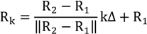
Let P(k), 1 ≤ k ≤ M be a set of estimates for the positions P(k) at position k. Let R
1 and R
2 be two reference points. Then arbitrary reference points can be created in between if these two points are connected by a linear belt and the positions R
1 and R
2 have been part of the calibration (For accuracy reasons). An interpolated reference point at position k with a step size of Δ is given by
The set P(k) includes all measurements at position k. Let
P(k) be the center of gravity for these points
The estimate of a systematic deviation b(k) is the distance between the reference point Rk and the center of gravity of the measurement points.
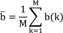
According to F.7a
b is calculated as
In this case the meaning of
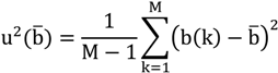
b is the mean systematic correction factor. The variance associated with
b can be calculated similar to F.7b as
The mean variance of the correction b(k) incorporates the uncertainty of the calibration and the uncertainty of the evaluation of b(k). Let u
1 and u
2 be the uncertainty of the reference points R
1 and R
2. Assuming a simple linear interpolation the uncertainty for the point R
k is given as
Similar to F.7c we can now calculate the mean variance of the correction factor b(k) as
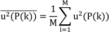
Using F.7d allows us to calculate the mean variance of each measurement. This variance is closely related to the DOP as it just defines the spread of the points at each position.
Finally the single value for the combined standard uncertainty is
Reporting results as in Equation (14) is necessary as the positions are 3-dimensional quantities but the distance is only a scalar. A possible extension for the formalism applied here would be to define all equations in all three dimensions. The benefit of such approach would be that the results would also include some information about the direction of the error components. For the systematic effect, this would give information if measurements are for example just parallel shifted to the reference path or a more complex effect applies. For the random component, this would allow an interpretation similar to the horizontal DOP (HDOP) or vertical DOP (VDOP). The drawback is that multiple values are more difficult to compare and interpret.
5.6. Temperature Compensation during Operation
Localization is performed by TDoA and therefore Equation (12) applies. It can be seen that there is no systematic error component with the exception of the temperature. For the best approach it is suggested that at least on receiver, already used within the calibration, is kept for the full system life time. The design of LOSNUS actually favors such an approach as adding more receivers does not in any case reduce measurement frequency. In addition, the cost increase is minimal.
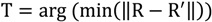
If such a receiver R exists and we have three time differences the receiver can be located by the transmitters using a multilateration equation. Such a function requires four transmitter positions assumed without loss of generality as T1, T2, T3, T4, three time differences t12, t13, t14 and the temperature T for calculating speed of sound.
Assume for now that there is no error component in the time differences. What we know is that the receiver should still be at the same position obtained during calibration. If this is not the case then T must be wrong. Therefore, the correct temperature T is the one which minimizes
5.7. Impact of Motion and Doppler Effect
Doppler Effect is noticeable when either the transmitting or receiving device is in motion. In the LPS
LOSNUS, only the receiver is in motion and the transmitters are fixed. If the chirp is centered at a carrier frequency f
0 the Doppler shift can be approximated by [
31] where
![Ijgi 02 00908 i035]()
is the direction and speed of motion of the receiver R. The direction of wave propagation between the transmitter and receiver is given by the unity vector
![Ijgi 02 00908 i036]()
.
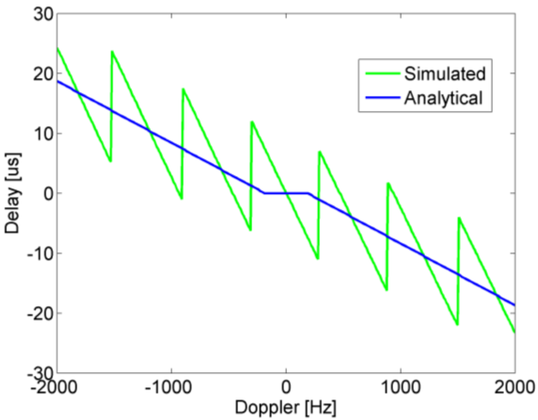
The effect of Doppler for a linear frequency modulated chirp with the settings of
Figure 3 has been evaluated using an analytical formula from ([
30], p. 210) and by a simulation. The effect on the peak of the correlation amplitude is neglect able and the time shift due to the Doppler effect is shown in
Figure 9.
Figure 9.
Time delays due to Doppler shifts for analytical function and simulation.
Figure 9.
Time delays due to Doppler shifts for analytical function and simulation.
Using the result from
Figure 9, the effect of Doppler shifts and motion on localization can be calculated. If a sound wave is emitted at time t = 0 and the receiver is moving in direction
![Ijgi 02 00908 i037]()
the solution of the Equation (31) determines the ToF.
As the node is moving and the distances to all transmitters are typically different, what is meant with by the value of the position of the receiver must be defined. In this article, the position of the receiver is defined as the position where the first transmitting signal within a locating sequence has been received. This definition was chosen for the following reasons: (a) without additional measures the receiver does not know in which direction it is moving. (b) It is logical to timestamp the position with the timestamp when the locating sequence starts. This position is denoted by R0. The error for a located position R can therefore be defined according to Equation (32).
Figure 10a,b show locating errors for different receiver velocities and interframe spacings. The values have been calculated by simulation using uniformly spaced receivers within the room. For each receiver all six possible directions of movement have been evaluated. For a given velocity, the value of the curve represents the mean error over all receiver positions where the error bar represents the standard deviation. As a general result, the system works well in this configuration up to target velocities of 0.5 m/s where the effect of Doppler is existent but not significant. Increasing the inter frame spacing worsens the result although at receiver velocities high than 0.5 m/s both systems experience problems.
Figure 10.
Simulation Results: (a) Effect of receiver motion with 0 ms interface spacing (only possible in CDMA system), (b) Effect of receiver motion with 10 ms interframe spacing suitable for LPS LOSNUS with up to 3.4 m minimal spacing between consecutively firing transmitters.
Figure 10.
Simulation Results: (a) Effect of receiver motion with 0 ms interface spacing (only possible in CDMA system), (b) Effect of receiver motion with 10 ms interframe spacing suitable for LPS LOSNUS with up to 3.4 m minimal spacing between consecutively firing transmitters.
6. Experimental Results
6.1. System Configuration
The LPS
LOSNUS system is installed in a 4 × 6 × 4 m testing room. The room closely reassembles a standard office room including tables, chairs and other instruments. The system can tolerate a single ToA error and includes six transmitters and up to eight receivers. The transmitters used are Senscomp 600 environmental grade electrostatic transducers with a large bandwidth and good acoustic coupling to air due to their low acoustic impedance. At the test system, these transmitters are mounted on the wall and their positions relative to the system of coordinates are marked in
Figure 11a. Transmitters can be adjusted in two directions as shown in
Figure 11b. All transmitters are wired to an activation unit controlled by a PC with a NI-DAQ card containing digital outputs for selecting the corresponding transmitter and an arbitrary waveform generator (AWG) shown in
Figure 12. A high voltage (HV) amplifier amplifies the AWG output.
Figure 11.
(a) Test system configuration consisting of six US transmitters. (b) Ultrasonic transmitter adjustable in two direction including wiring.
Figure 11.
(a) Test system configuration consisting of six US transmitters. (b) Ultrasonic transmitter adjustable in two direction including wiring.
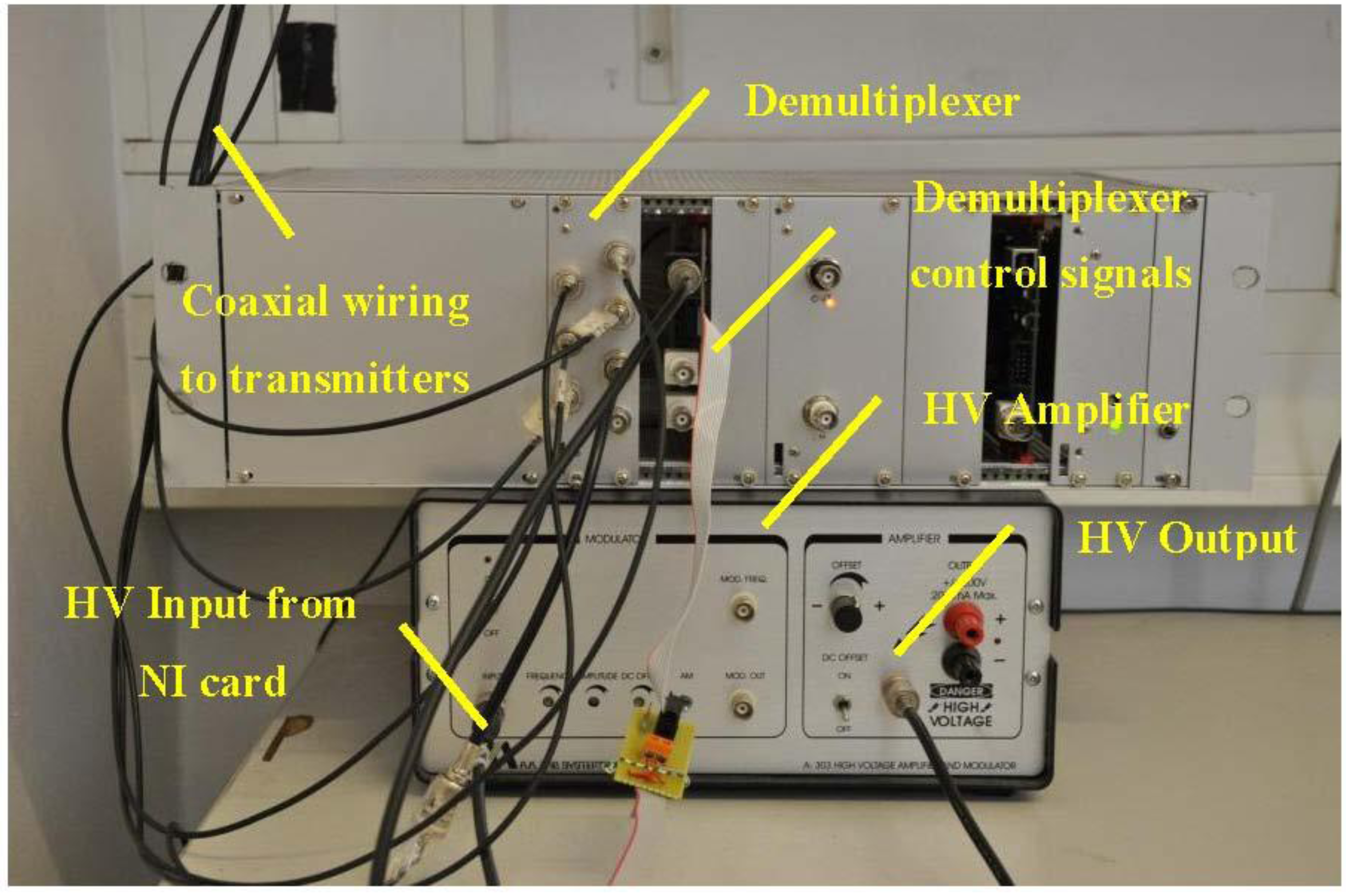
Figure 12.
Activation unit consisting of high voltage (HV) amplifier, demultiplexer and cabling.
Figure 12.
Activation unit consisting of high voltage (HV) amplifier, demultiplexer and cabling.
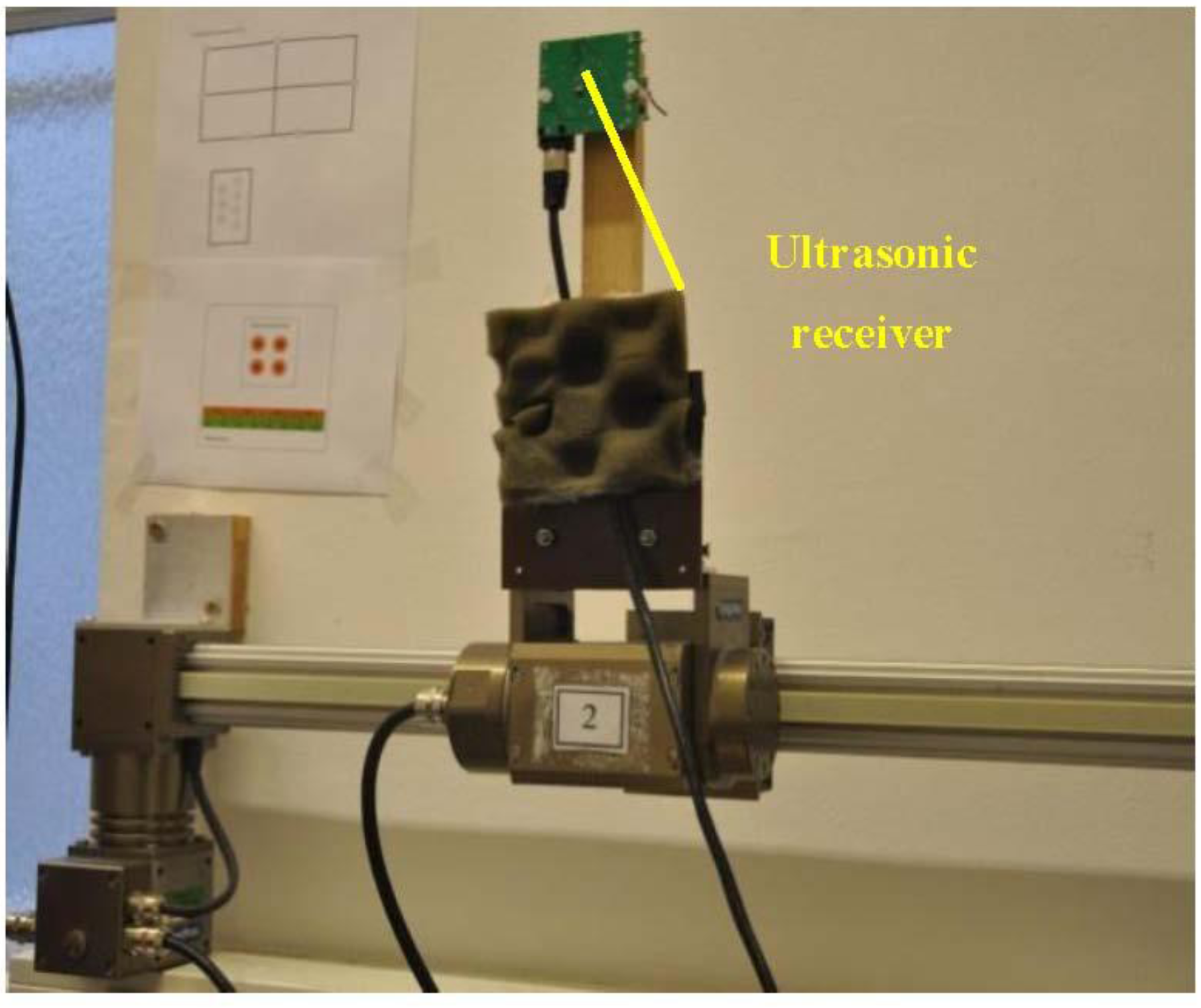
The receivers for calibration and verification are positioned on the opposite side with a distance of approx. 3 to 4 m. A linear moving axis with a length of 1.5 m mounted at a height of approx. 1 m enables tests with moving devices and can be used for judging the quality of the localization and the calibration. The setup for the linear belt including the receiver is shown in
Figure 13. The outputs of the receivers are also wired to the NI-DAQ card through a mixer module, which can be used to extend the number of channels to eight. For practical use of the LPS, small embedded sensor nodes and low cost devices were also built by the authors. They deliver the same performance but aim at reducing costs and size of sensor nodes.
Figure 13.
Receiver unit mounted on moving belt.
Figure 13.
Receiver unit mounted on moving belt.
6.2. Calibration
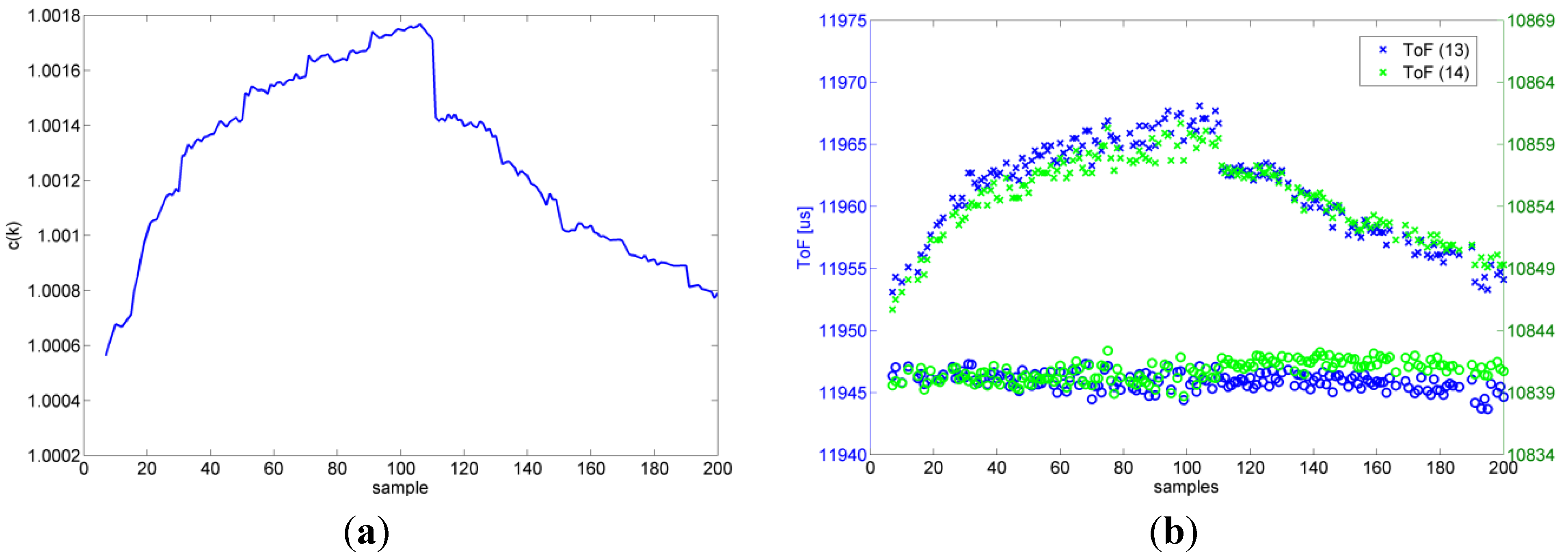
For the calibration, we used six transmitters and seven receivers although only four transmitters would have been required. The additional ones are used for verification and cross checking. In addition, one of the seven receivers was mounted on a linear belt where two positions have been used during the calibration process. These positions will be used as reference positions later on, as they have a known uncertainty. In total, a measurement at each position delivers 48 ToF values. As the measurements including the belt movement require some time, the assumption of a constant temperature is not sound anymore and a compensation approach has to be used. Applying the compensation algorithm of Equation (10) where the sum of ToF is kept constant a compensation curve shown in
Figure 14a is obtained. An example for two compensated ToF measurements is shown in
Figure 14b.
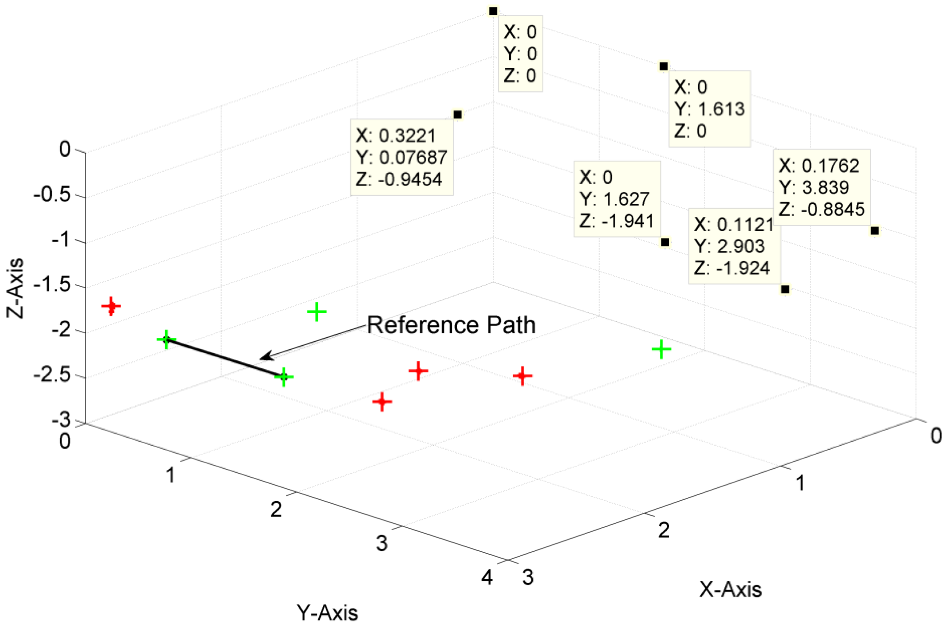
The post processed averaged data is used as input for the calibration algorithm. Another input is an initial guess of transmitters and receivers positions, the speed of sound and the acoustical delay due to the cones, which are required for broad coverage. The final output of the calibration algorithm is then scaled to the length of the reference path. The three dimensional calibration results are shown in
Figure 15 and
Table 1. The transmitters are marked with their x/y/z coordinates, the green symbols are the receivers used within the calibration process and the red symbols are located but unused receivers within the localization process. The reference path between the receivers is shown as a line between the two receivers. Comparing the result manually with the real transmitter and receiver positions shows feasible results. However judging the calibration result is not possible in this way with sufficient quality. Using the proposed method, which includes a reference path, eases this task as uncertainty of the calibration is well defined.
Figure 14.
(a) Compensation factor c(k) calculated according to Equation (10); (b) Example of two ToFs compensated with factor c(k). Data points marked with “x” are before compensation and data points marked with “o” are after compensation.
Figure 14.
(a) Compensation factor c(k) calculated according to Equation (10); (b) Example of two ToFs compensated with factor c(k). Data points marked with “x” are before compensation and data points marked with “o” are after compensation.
Figure 15.
Calibration result (a = 1.012, time delay cone = 81.2 µs, c = 347.3 m/s).
Figure 15.
Calibration result (a = 1.012, time delay cone = 81.2 µs, c = 347.3 m/s).
Table 1.
Calibrated transmitter positions (in meters).
Table 1.
Calibrated transmitter positions (in meters).
| | Tx1 | Tx2 | Tx3 | Tx4 | Tx5 | Tx6 |
|---|
| x | 0 | 0 | 0.3221 | 0 | 0.1121 | 0.1762 |
| y | 1.6126 | 0 | 0.0769 | 1.6271 | 2.903 | 3.8394 |
| z | 0 | 0 | −0.9454 | −1.9408 | −1.9240 | −0.8845 |
6.3. Localization
In the operating phase of
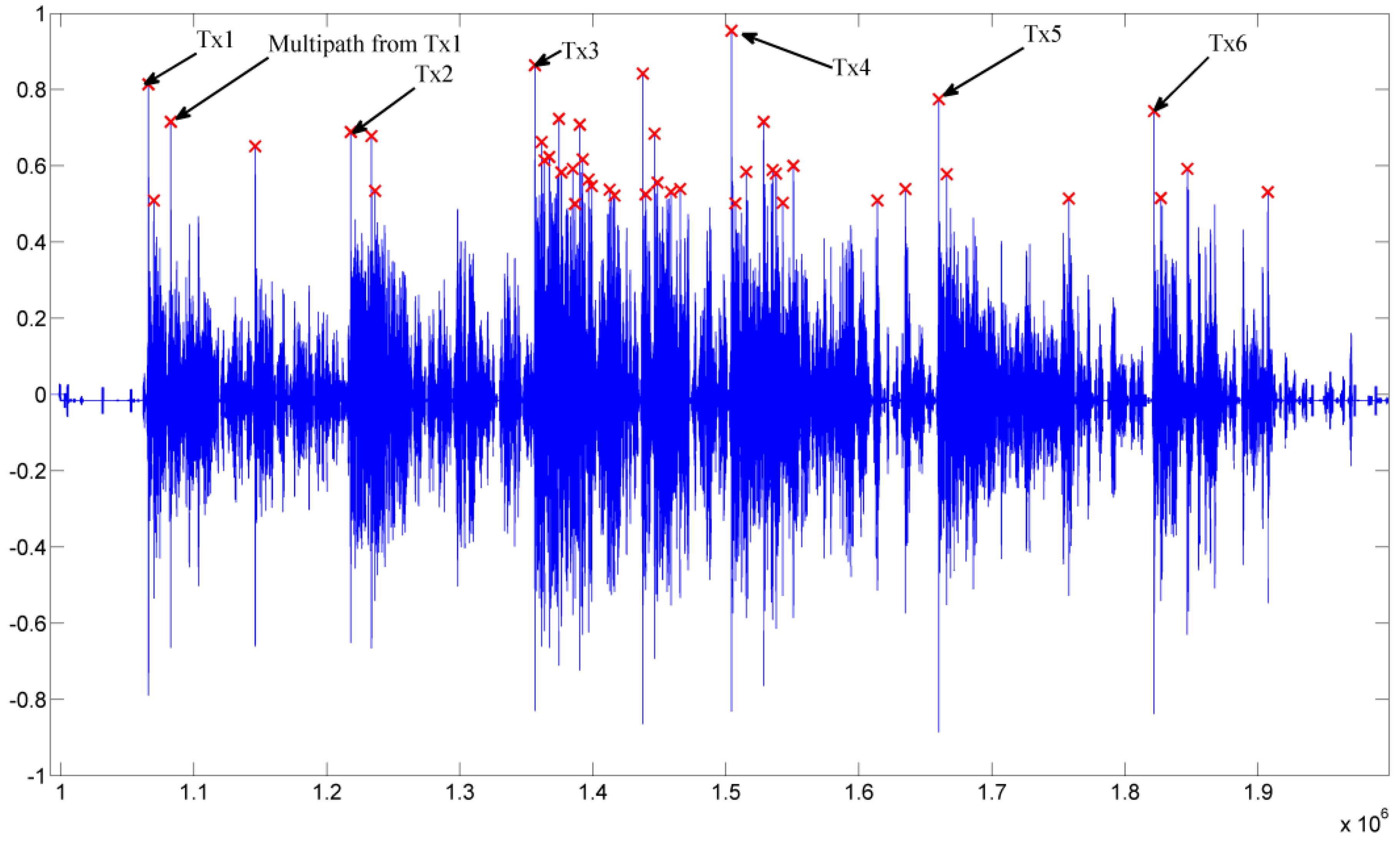
LOSNUS, the transmitter positions obtained by the calibration process are used for device localization by TDoA. Locating is started by sequentially firing the transmitters with the well-defined protocol. For every transmitter a frame including its unique transmitter coding frequency is sent. Such signals are then received by ultrasonic receivers of the devices and processed by binary cross correlation. An example of a correlation result is shown in
Figure 16. A typical correlation result includes several peaks. The first peak of each transmitter coding is considered to be the LoS, which gives the correct ToA values. These ToA values are then evaluated using the proposed locating algorithm.
Figure 16.
Correlation results of a complete LOSNUS sequence showing ToA for individual transmitters and an example for a Non Line of Sight (NLOS) signal for Tx1.
Figure 16.
Correlation results of a complete LOSNUS sequence showing ToA for individual transmitters and an example for a Non Line of Sight (NLOS) signal for Tx1.
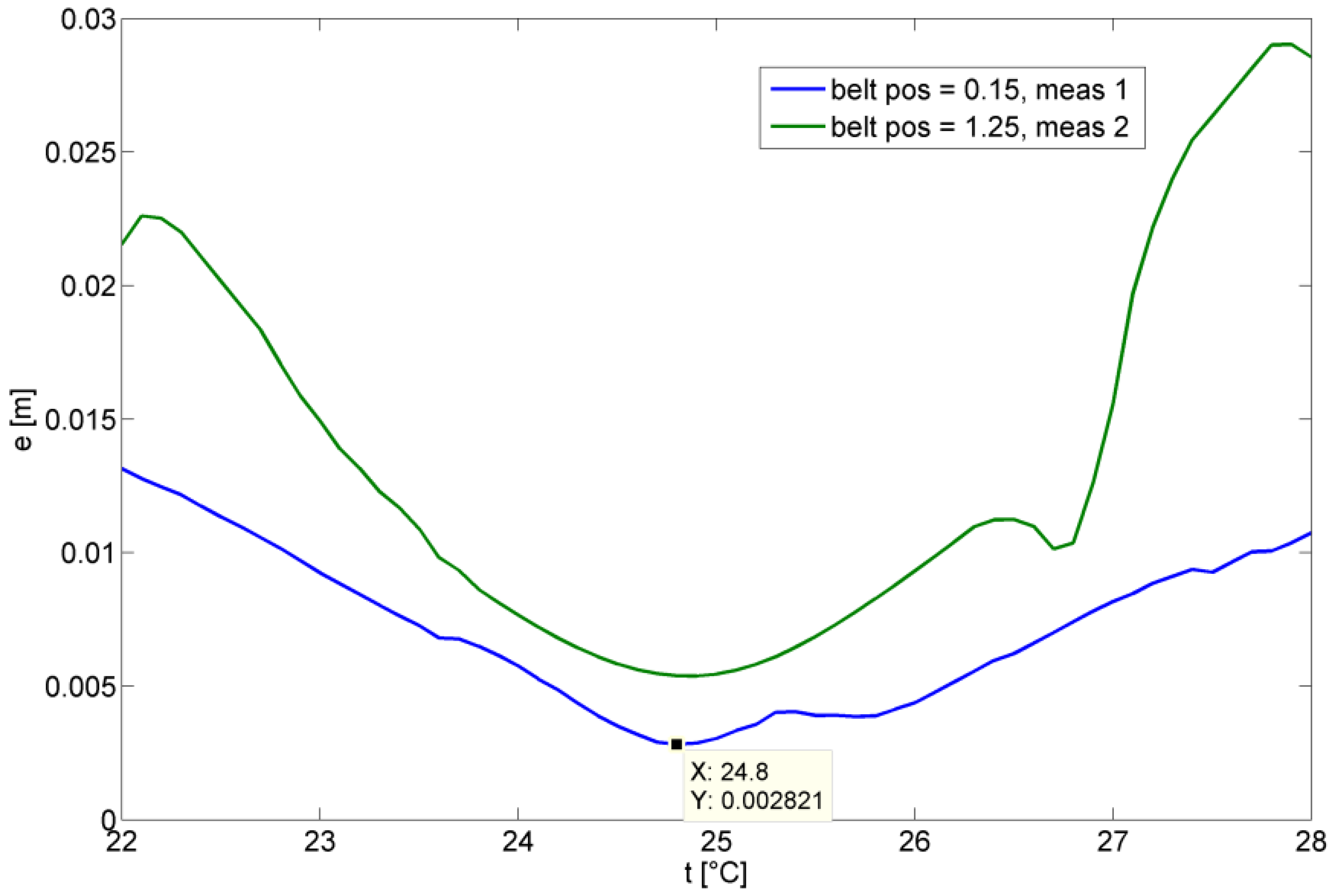
23 positions have been measured on the belt with a spacing of 50 mm. At each position, 20 measurements have been taken. The start and the end positions are also the reference positions used within the calibration. In the first step, the correct temperature has been estimated using Equation (29) using the fact that the reference position cannot move. This is shown in
Figure 17 where the mean deviation of the 20 measurements at the reference point is shown for different temperature values. The correct temperature is 24.8° which is in close agreement with the manually measured temperature of 24.9°.
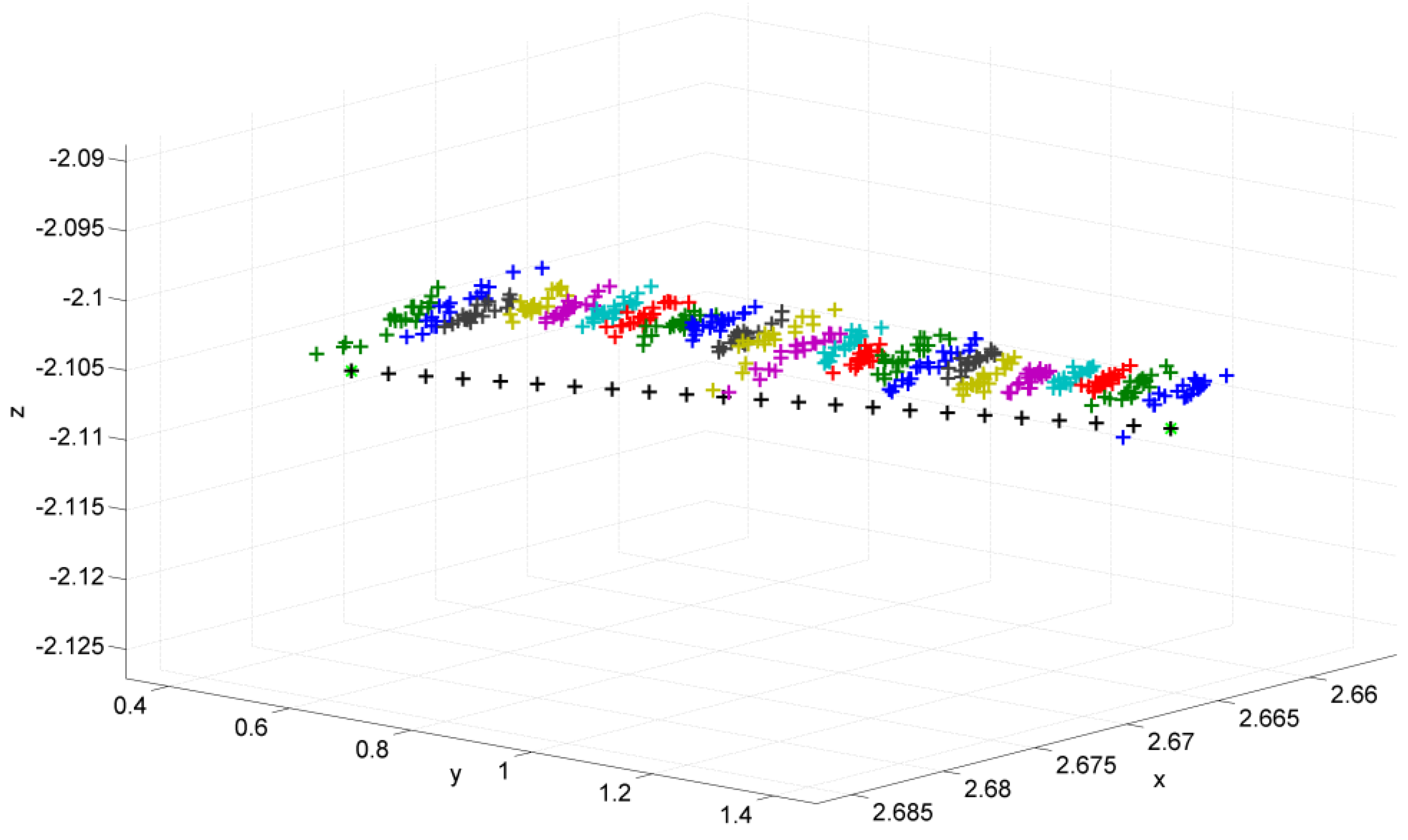
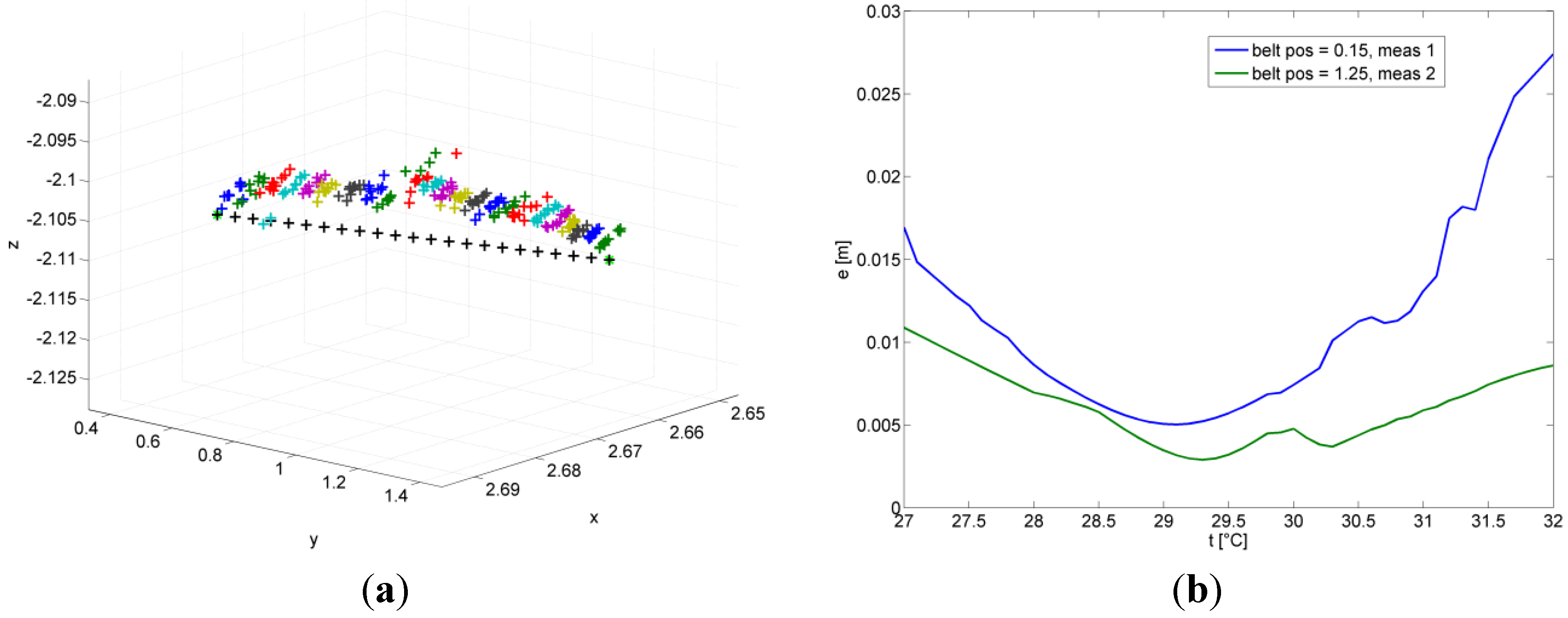
The measurements are shown in
Figure 18. The two green star symbols are the reference positions from the calibration. The black plus symbols are the interpolated reference positions modeling the linear belt. At each position, a group of 20 measurements can be seen where the spread is a result of the DOP and the uncertainty of the TDoA measurement. The distance of the mean to the reference positions is due to the temperature uncertainty and calibration uncertainty. Anyhow the result is remarkable where standard uncertainty for this measurement is reported as ||P − (x, y, z)
T|| = 4.7 mm ± 1.3 mm. A graphical visualization of the uncertainty components is shown in
Figure 19a. In this case b(k) calculated according to Equation (18) shows the systematic component of the uncertainty,
i.e., the mean distance between the points and the reference position. The value of
![Ijgi 02 00908 i038]()
is the standard deviation of the measured points at position k. This value is closely related to the DOP by the standard deviation of the ToA measurements and the DOP for the transmitter/receiver combination used. Due to the large and accurate reference path used the component
![Ijgi 02 00908 i039]()
is rather small.
Figure 17.
Determination of temperature using reference positions.
Figure 17.
Determination of temperature using reference positions.
Figure 18.
Measurement on linear belt at 23 positions with 20 measurements each. Temperature = 24.8 °C taken from
Figure 17.
Figure 18.
Measurement on linear belt at 23 positions with 20 measurements each. Temperature = 24.8 °C taken from
Figure 17.
What is also interesting to point out is that the final result did not contain any outlier (no postprocessing was performed on the input data). This is also a remarkable as at about 0.6 m on the belt the signal for transmitter six is lost. This is shown in
Figure 19b.
Reproducibility under different environmental conditions was verified as well. Again temperature identification shown in
Figure 20b and results shown in
Figure 20a are good. The reported standard uncertainty is ||P − (x, y, z)
T|| = 6 mm ± 2.2 mm. The deviations between the two results, although small, are due to the finite sample size. In addition modeling does not take into account all possible effects.
Figure 19.
(a) Mean error from reference points; (b) Size of groups at different positions.
Figure 19.
(a) Mean error from reference points; (b) Size of groups at different positions.
Figure 20.
(a) Repeated measurement at different date and temperature; (b) Temperature obtained by using reference position was 29.1 °C.
Figure 20.
(a) Repeated measurement at different date and temperature; (b) Temperature obtained by using reference position was 29.1 °C.
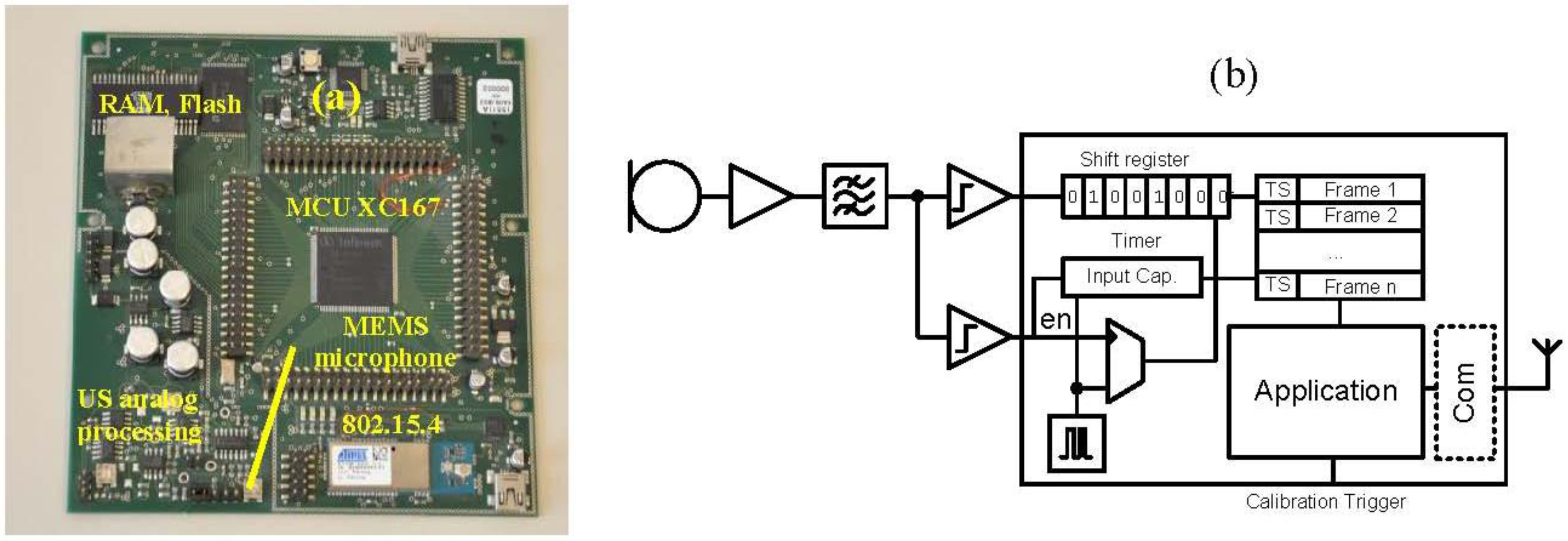
6.4. Practical Realization Considerations
Figure 21a shows a realization of an ultrasonic receiver using a low cost microcontroller, a MEMS microphone and a ZigBee controller for data communication. The suggested software architecture is shown in
Figure 21b. The input signal is amplified and bandpass filtered. Further processing is performed 1-bit only. Two operating modes are possible. In a low power mode the ultrasonic receiver is activated by the startframe available in the
LOSNUS sequence. If a lead-in is received, the lower comparator triggers the input capture register storing the current time of the free running clock and starts clocking the shift register. Storing of a frame stops if no further input condition is present and the total frame length has elapsed. A typical length of the frame including lead-in, chirp and transmitter coding at 1 MS is small and requires 740 Bit. These frames can then be processed offline.
Figure 21.
(a) Picture showing a test realization of a sensor node with a ZigBee communication interface. (b) Suggested software architecture for implementation.
Figure 21.
(a) Picture showing a test realization of a sensor node with a ZigBee communication interface. (b) Suggested software architecture for implementation.
The other operating mode is when the shift register is permanently clocked and correlation with the chirp is always performed. In this case neither the starting frame nor the comparator for enabling reception is necessary. This mode is useful when power consumption is not of concern and the system should operate at very low SNRs as pulse compression allows detection of frames with an SNR close to zero.
7. Conclusion
The article presented the LPS
LOSNUS, which is designed for numerous located devices, low cost, and high accuracy by an integrated concept of calibration and localization. A basic requirement for high accuracy is an accurate calibration, which is ensured by high quality ToF measurements and a known reference distance. Localization results are presented with respect to robustness and accuracy. A quantitative measure for accuracy is derived by application of the guidelines recommended by the GUM [
30]. This allows an individual assessment of systematic and random components and applying the results to different system configurations. Robustness is achieved by a novel clustering algorithm, which enables recognizing and eliminating a single non-line-of-sight error. Results have been presented for two different scenarios showing uncertainties less than 1 cm in all cases, which is a remarkable result. Ongoing work is concentrating on several practical aspects of the system, e.g., receiver clock correction and other methods of error reduction.


 be the transmitters,
 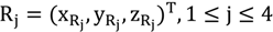 , c the speed of sound and tij be the ToF between transmitter i and receiver j. The defining equations are then given by


 is the direction and speed of motion of the receiver R. The direction of wave propagation between the transmitter and receiver is given by the unity vector
  .
.

 the solution of the Equation (31) determines the ToF.


 is the standard deviation of the measured points at position k. This value is closely related to the DOP by the standard deviation of the ToA measurements and the DOP for the transmitter/receiver combination used. Due to the large and accurate reference path used the component
  is rather small.