Abstract
On the route to a spatio-temporal geoscience information system, an appropriate data model for geo-objects in space and time has been developed. In this model, geo-objects are represented as sequences of geometries and properties with continuous evolution in each time interval. Because geomodeling software systems usually model objects at specific time instances, we want to interpolate the geometry and properties from two models of an object with only geometrical constraints (no physical or mechanical constraints). This process is called spatio-temporal data construction or morphological interpolation of intermediate geometries. This paper is strictly related to shape morphing, shape deformation, cross-parameterization and compatible remeshing and is only concerned with geological surfaces. In this study, two main sub-solutions construct compatible meshes and find trajectories in which vertices of the mesh evolve. This research aims to find an algorithm to construct spatio-temporal data with some constraints from the geosciences, such as cutting surfaces by faulting or fracturing phenomena and evolving boundaries attached to other surfaces. Another goal of this research is the implementation of the algorithm in a software product, namely a gOcad plug-in. The four main procedures of the algorithm are cutting the surfaces, setting up constraints, partitioning and calculating the parameterizations and trajectories. The software has been tested to construct data for a salt dome and other surfaces in regard to the geological processes of faulting, deposition and erosion. The result of this research is an algorithm and software for the construction of spatio-temporal data.
1. Introduction
Because the geosciences field examines spatial and temporal changes in the Earth, integration of spatial and temporal data is a natural requirement of many applications in the geosciences. So far, three-dimensional (3D) spatial data have been well integrated in the geosciences, though the integration of temporal data has not gained much success, because of its complexity. Our work aims to overcome this complexity by reviewing concepts, developing a data model and building software and applications. Through this approach, we have developed an appropriate data model [1], in which we considered a real time axis. This time axis was subdivided into intervals, and it requires that geometry and geoscience properties be changed continuously throughout the time intervals.
Because geomodeling software systems usually model objects at specific time instances, this research aims to interpolate intermediate geometries or find an algorithm to construct data in each time interval [ti, ti + 1] from two input data models at time ti and time ti + 1. This paper is motivated by the requirement of capturing data for a spatio-temporal geoscience information system with the capability of processing and answering queries, such as: “Given a location (geo-object at a specified location) and properties, such as temperature and pressure, for what period(s) of time was the geo-object exposed to the location and the properties?” or “What are the geometry and properties of a geo-object at a given time?”
We assume that in a small enough time interval, a geological layer, which is subjected to deposition, erosion and uplift, is changing smoothly and regularly. Thus, the constructed data represent the temporal evolution of a geo-object. Therefore, the construction process is called spatio-temporal data construction. The algorithm also considers several geometrical constraints that enable the modeled evolution to be closer to the “true” historical evolution. To simplify the problem of spatio-temporal data integration, only three-dimensional triangle meshes are considered. Solid and other types of geo-objects will be considered in our future work.
Some studies exist regarding morphological interpolation based on mathematical morphology [2,3,4,5]. These methods were restricted to images (binary/grayscale and color) and were used to generate intermediate 2D sections and to reconstruct 3D objects from their initial 2D sections. These studies differ significantly from our study; we constructed 4D objects from 3D mesh surfaces at each time instance.
The algorithm is based on parameterization techniques and is comprised of four procedures: the cutting procedure, the setting up constraints procedure, the partition procedure and the calculation of parameterizations and trajectories procedure. The algorithm is implemented as a gOcad plug-in and is tested with the data construction of a salt dome and other surfaces in regard to their faulting, deposition and erosion processes.
2. Related Work
This research is strictly related to shape morphing, shape deformation, cross-parameterization, compatible meshing, two-dimensional or three-dimensional parameterization in areas of computer graphics and computer-aided geometric design. These techniques have received much attention from researchers, such as Michael S. Floater [6,7,8,9], Bruno Lévy [10], Kai Hormann, Konrad Polthier, Alla Sheffer [11], Yaron Lipman [12], Xin Li [13], etc.
The shape morphing process contains two steps. The first step looks for a bijective map between the source shape and the target shape, known as the vertex correspondence or the consistent/compatible meshes. The second step chooses a set of trajectories, along which the corresponding vertices travel as they evolve from the first set of vertices into the second set of vertices. This process is known as the vertex path/trajectory [6,14,15,16]. Regarding the first step, Van Kaick et al. [17] provides a good recent review of compatible triangle meshes. The compatible meshes are typically computed by first subdividing two meshes into corresponding patches, which are homeomorphic to disks; secondly, the parameterization of the two meshes on a common base domain is calculated. Thirdly, the cross-parameterization is calculated, and finally, the meshes are remeshed [18,19]. Following this framework, our algorithm creates compatible meshes. Moreover, we incorporate the cutting procedure to make it suitable for application in the geosciences field. A summary of mesh parameterization techniques is given in [10,11]. Some factors should be considered when using a parameterization, such as distortion, bijectivity, freedom of boundary and complexity. In our algorithm, mean value parameterization is chosen, because of the bijection and fixed-boundary properties of this technique; hence, we maintain consistency in the boundaries of the patches.
Most of the morphing techniques do not concern the second step in the shape morphing process, but solve the first step in the shape morphing process and then use linear trajectories, i.e., the straight-line segments of the corresponding vertices. M.S. Floater used convex combinations for trajectories [6]. Finding trajectories by moving a rigid shape (or as rigid as possible) is described in [14,16]. Using strain fields to choose trajectories is described in [15]. In our algorithm, the finding trajectories’ sub-procedure is built on the convex combination method, as described in [6], with the assumption that intermediate surfaces have a “combinatorial” property, i.e., every interior vertex can be represented as a convex combination of its neighbor.
3. Methodology
Let M be a three-dimensional triangle mesh in ℝ3. Methods to represent a mesh have been developed, with examples described in [10]. In short, we consider a mesh to be a pair of a sequence of its vertices and its topology, M = (V,T). V is a sequence of n distinct points, vi = (xi,yi,zi) in ℝ3. V can also be considered a map from the index set, I = {1…n} to ℝ3, where V(i) = vi for all i = 1, …, n. T is the topology or the structure of the mesh entirely defined on the index set, I. The topology defines the set of triangles or faces, the set of edges, the set of boundaries and the set of interior/boundary vertices of the mesh.
We construct data in the time interval, [ti, ti + 1], from data at time instances, ti and ti + 1, by smoothly changing a source mesh into a target mesh. Choosing data at ti as the source mesh and data at ti + 1 as the target mesh, or vice versa, depends on the user. However, our algorithm is designed in a way that it will become faster (because cutting paths are not required in the target mesh) when the more complicated mesh is chosen as the source mesh. We always denote the source mesh as Ms and the target mesh as Mt. The following paragraphs define some of the special terms used in the paper.
A control vertex of the mesh, M(V,T), is a user-selected vertex, vi ∈ V. A path in mesh M(V,T) is a sequence (νp1, νp2, …, νph), where pi ∈ I and [νpi, νpi + 1] is an edge of M for all i = 1, …, h − 1. A Boundary path is a path in which all of its vertices are in the boundaries. The cutting path and fence path are paths used in the cutting procedure and the partition procedure, respectively.
A unit regular k-polygon, k ≥ 3, is a simple polygon with k vertices in a certain plane, such that coordinates of its vertices are defined by the formula, 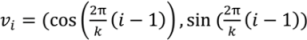 , for all i in {1…k}.
, for all i in {1…k}.The error, ε(M,N), between two meshes, M and N, is defined by the form, ε(M,N) = max(max(dist(x, N):x ∈ VMI), max(dist(x,M),:x ∈ VNI)), where VMI is a set of interior vertices of M, VNI is a set of interior vertices of N and dist(x,L) (the distance between a point, p, and a mesh, L) is the minimum distance between the point, p, and those in L. Note that in this term, we consider only interior vertices, not boundary vertices.
Definition 1. Two meshes, M(V,T) and N(U,G), are compatible, if (i) V and U have the same total number of vertices and they are corresponding in their order, i.e., a trivial map, h, exists, such that h(vi) = ui for all i = 1, …, n; and (ii) T = G.
Definition 2. Given m ≥ 2 and an n-vertices mesh, M(V,T), trajectories of the mesh, M(V,T), that represent its continuous evolution into its compatible mesh, N(U,T), are n distinct line strings, such that for each line string, m vertices exist, i.e., the ith line string, 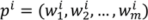 , and
, and  ,
,  for all i = 1, …, n.
, and , for all i = 1, …, n.Definition 3. Given m ≥ 2, an n-vertices mesh, M(V,T) and its compatible mesh, N(U,T), linear trajectories of the mesh, M(V,T), are trajectories of M, where each vertex of a trajectory, , is defined as 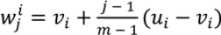 for all i = 1, …, n; j = 1, …, m.
, is defined as for all i = 1, …, n; j = 1, …, m.Figure 1 presents a block diagram of our algorithm containing the four main procedures. First, the cutting procedure adds “missing” boundaries to the meshes, such that the error between the old and new meshes is zero. Second, the setting up constraints procedure sets up control vertices, the pairs of control vertices between the source mesh and the target mesh, fence paths and the attaching constraints of boundary vertices. Third, the partition procedure subdivides the source mesh and the target mesh into corresponding pairs of source patches and target patches, such that every patch is homeomorphic to a disk. Fourth, the calculating procedure calculates cross-parameterization, generates compatible meshes and finds trajectories for each pair of patches. Finally, these results are combined to achieve the final result for the original source mesh and the original target mesh. The first two procedures are user interactive procedures, while the last two are automatic. Moreover, the first two create input data for the last two.
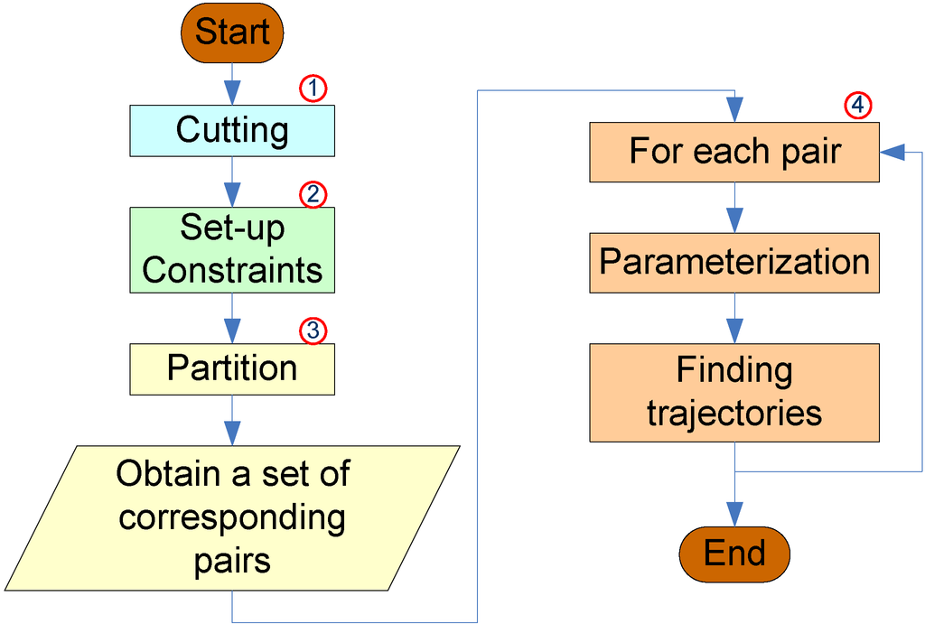
Figure 1.
The block diagram of the algorithm.
Figure 1.
The block diagram of the algorithm.

3.1. Cutting
Missing boundaries of the source mesh and the target mesh exist, due to the faulting or fracturing phenomena. Cutting paths are created to represent these missing boundaries. They are created in the source mesh to represent naturally occurring faults or fractures that first begin appearing in the source surface and then evolve into fractures in the target surface. Cutting paths are not required to be created in the target mesh to represent faults or fractures already existing in the source surface and evolving to disappear in the target surface. In the latter situation where cutting paths are not required, fence paths are created instead.
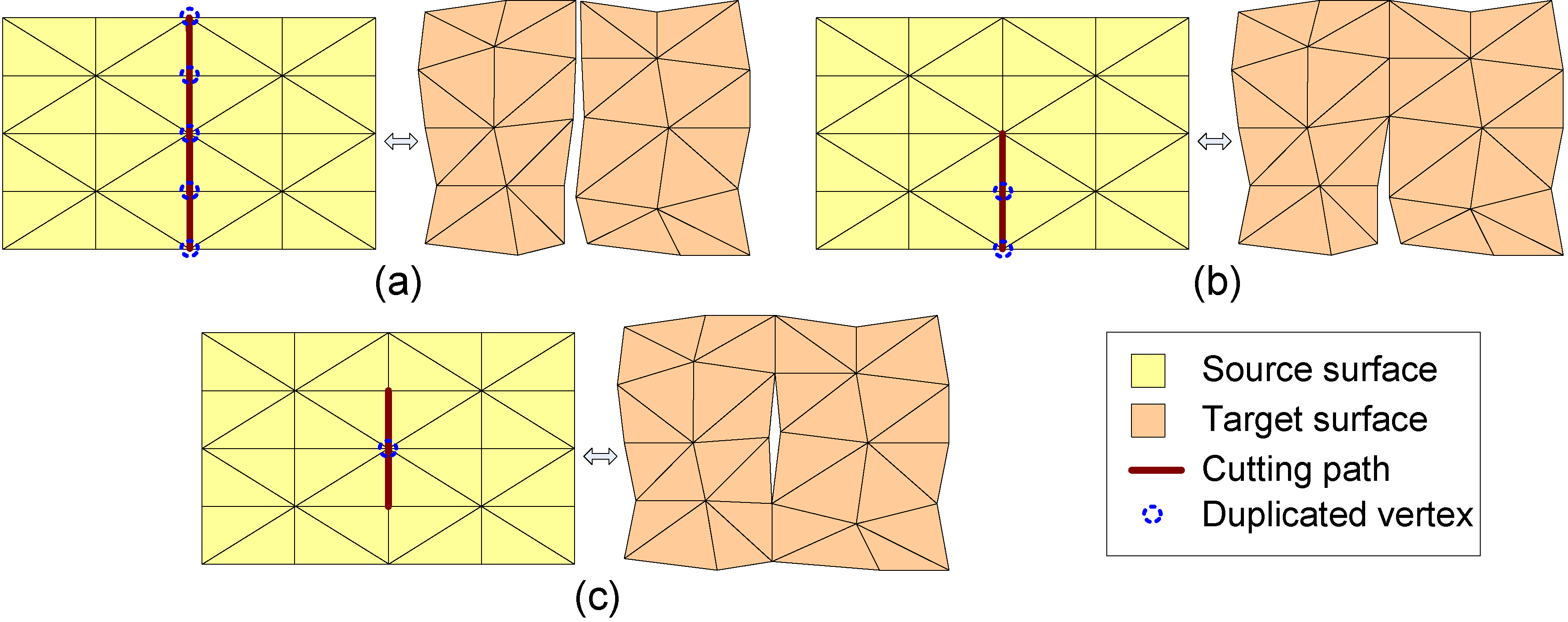
Let P be a set of user-selected cutting paths in M. This procedure cuts the mesh, M, by P. Three types of cutting paths are supported, as shown in Figure 2. All vertices and edges of cutting paths are duplicated (as in Figure 2a), except for a one-end vertex (as in Figure 2b) or two-end vertices (as in Figure 2c). Blue dashed circles represent duplicated vertices.

Figure 2.
Cutting meshes by cutting paths. (a) All vertices and edges are duplicated. (b) All vertices and edges, except for a one-end vertex, are duplicated. (c) All vertices and edges, except for two-end vertices, are duplicated.
Figure 2.
Cutting meshes by cutting paths. (a) All vertices and edges are duplicated. (b) All vertices and edges, except for a one-end vertex, are duplicated. (c) All vertices and edges, except for two-end vertices, are duplicated.
Because the procedure is completed as described above, the error between the old mesh and the new mesh is zero. After this procedure, we still denote Ms and Mt as the source mesh and the target mesh, respectively.
3.2. Setting up Constraints
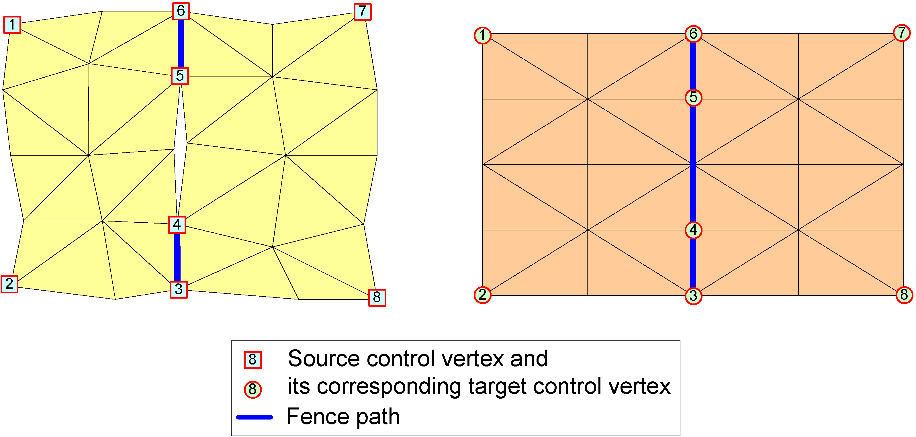
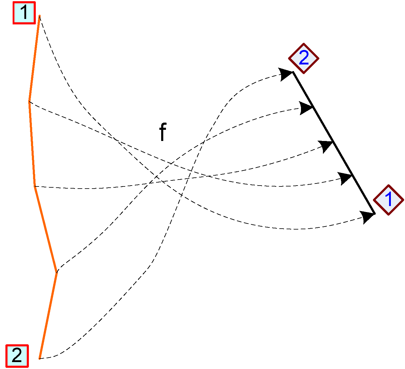
Our algorithm uses four types of constraints: control vertex, control vertex pair, fence path, and attaching constraint. The user selects all of the constraints manually with an automatic tool, such as finding the shortest path between two-end vertices. Control vertices and control vertex pairs present fixed (known) corresponding vertices and are used to control the correspondence of other vertices. Control vertices are often corner vertices. The control vertices in the source mesh and the target mesh are represented by two sequences of control vertices, Vc and Wc, respectively, such that they deduce control vertex pairs by their order, i.e., (vc,i, wc,i) is a control vertex pair. Fence paths are used to alter cutting paths in the target mesh or to partition the source mesh and the target mesh into patches that are homeomorphic to disks. Fence paths are required to connect exactly two control vertices, for example, a fence path with h vertices in the source mesh, Ms, p(νp1, νp2, …, νph), satisfies the following conditions: vp1, vph ∈ Vc and vpi ∉ Vc for all i = 2, …, h − 1. All fence paths of the source mesh or target mesh cut each other only at their end vertices. Figure 3 depicts an example of control vertices, control vertex pairs (by corresponding order) and fence paths.
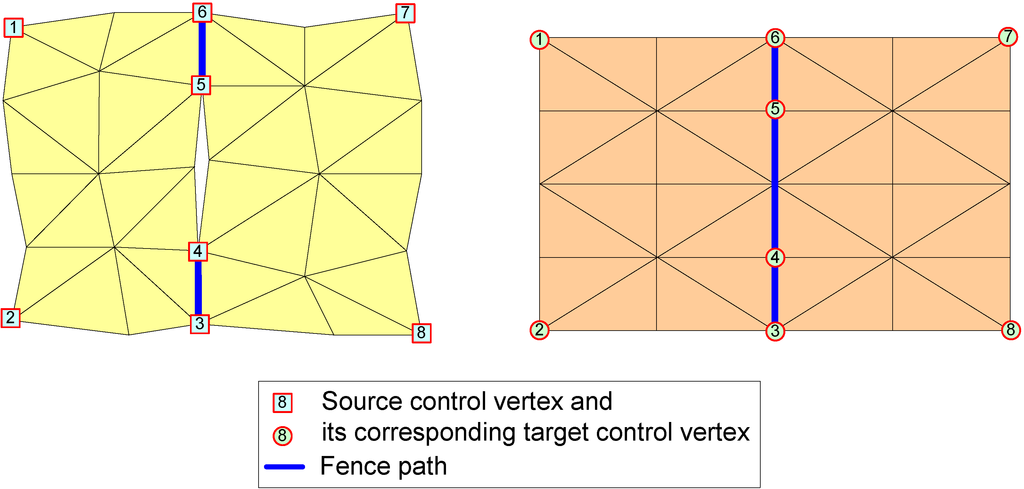
Figure 3.
An example of control vertices, control vertex pairs and fence paths.
Figure 3.
An example of control vertices, control vertex pairs and fence paths.
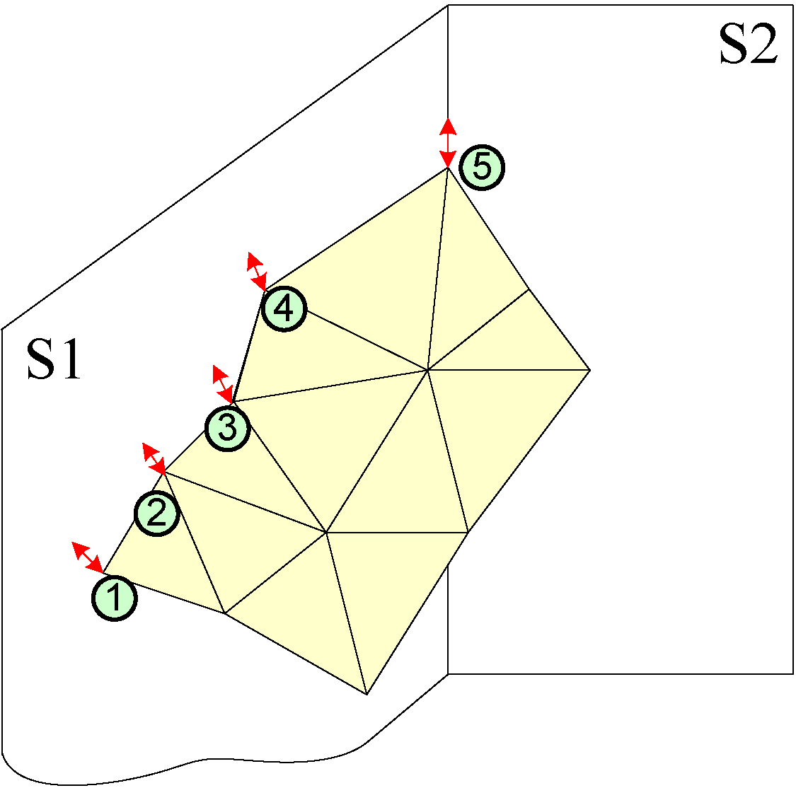
The attaching constraints present the adhesion of the vertices of the source mesh to the controlling surfaces during the evolution of the source mesh. If a 1-controlling surface attaching constraint is imposed on a vertex of the source mesh, this vertex will always be located on the controlling surface during its evolution. Similarly, if a 2-controlling surface attaching constraint is imposed on a vertex of the source mesh, this vertex will always be located on the line that is the intersection of the two controlling surfaces. In this paper, we delimit that the attaching constraints are only imposed on boundary vertices of the source mesh and that there are a maximum of two controlling surfaces involved in each attaching constraint. Furthermore, all vertices attached to two surfaces must be control vertices. Through these attaching constraints, each boundary vertex of the source mesh attaches to no surface, one surface or two surfaces. Figure 4 presents an example of attaching constraints. In this figure, boundary vertices, 1, 2, 3 and 4, attach to one surface (S1), (i.e., 1-controlling surface attaching constraint), boundary vertex 5 attaches to two surfaces (S1, S2), (i.e., 2-controlling surface attaching constraint) and the other boundary vertices do not attach to any surface, meaning that there are no attaching constraints imposed on these boundary vertices.

Figure 4.
An example of attaching constraints.
Figure 4.
An example of attaching constraints.
3.3. Partition
This procedure starts with the DefinePatches sub-procedure, dividing both the source mesh and the target mesh into patches by fence paths and their boundaries.
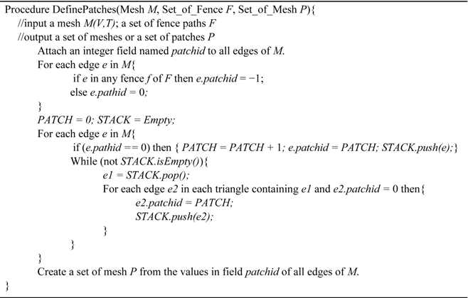
After the DefinePatches sub-procedure, the source mesh and the target mesh are partitioned into two sets of patches. This sub-procedure is consistently successful for any type of mesh and set of fence paths. Next, we check if each patch contains at least three control vertices and that all control vertices are in its boundary. We also check if each patch is homeomorphic to a disk. If the check fails, the first two procedures, i.e., cutting and set-up constraints, need to be repeated. Some reasons for this failure are as follows: (1) there are too few control vertices; (2) there exists a control vertex, which is not on the boundaries or fence paths; or (3) a hole exists in a patch. The requirement of disk homeomorphism can be satisfied for any type of mesh through the cutting procedure.
After all of the above steps, meshes Ms and Mt are partitioned into the same number of patches, k. If this condition is not satisfied, all of the above steps need to be repeated to set up more fence paths. This condition can be satisfied for any type of mesh through the set of user-defined fence paths. Discovery of the corresponding patches is accomplished by identifying the control vertices and their order in each patch. The result of this step is a set of patch pairs (Pi,s, Pi,t) for all i in {1…k}. Once again, if such a set of patch pairs is not found, all of the above steps are repeated. The cause of this failure is the lack of correspondence between the control vertices. This step will be successful if the control vertices and their order are correct.
3.4. Calculating
In this procedure, we work with each source patch and its corresponding target patch pair, denoted by (Ls, Lt). This procedure contains two sub-procedures: calculating the cross-parameterization (or constructing compatible meshes) sub-procedure and the finding trajectories sub-procedure.
3.5. Calculating Cross-Parameterization or Constructing Compatible Meshes
This sub-procedure is used to construct a new mesh that is compatible with the source mesh and that approximates the target mesh. The new mesh and the source mesh are compatible in the sense of having one-to-one correspondence between their vertices, edges and faces (Definition 1). The new mesh and the target mesh are considered well approximated if the distance or the error between them is smaller than the user’s threshold. Splitting a few triangles of the source mesh will reduce the error between the new mesh and the target mesh. In the following paragraphs, more detailed descriptions of the algorithm are given.
Given two patches or triangle meshes, Ls(V,T), Lt(W,F), both are homeomorphic to disks. Let Ics = (ics,1…ics,k) and Ict = (ict,1…ict,k) be index sequences of k, k ≥ 3, with distinct control vertices in Ls and Lt, respectively; additionally, a correspondence exists between the index sequences by their order. All control vertices are in the boundary of their meshes and are in a clockwise or counterclockwise order. To construct compatible meshes, we first find a bijection between the two meshes and, then, construct a new mesh using this map.
In the first step, we map both patch boundaries to the boundary of a unit regular k-polygon using the “chord” length method for each boundary path (Figure 5), i.e., mapping f from a path, p(νp1, νp2, …, νph), with h vertices to a segment. s(x1, x2). of the unit regular k-polygon. This method is defined by the following formula: f(νp1) = x1; 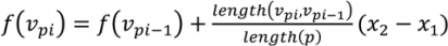 for all i in 2, …, h, where
  .
.
for all i in 2, …, h, where .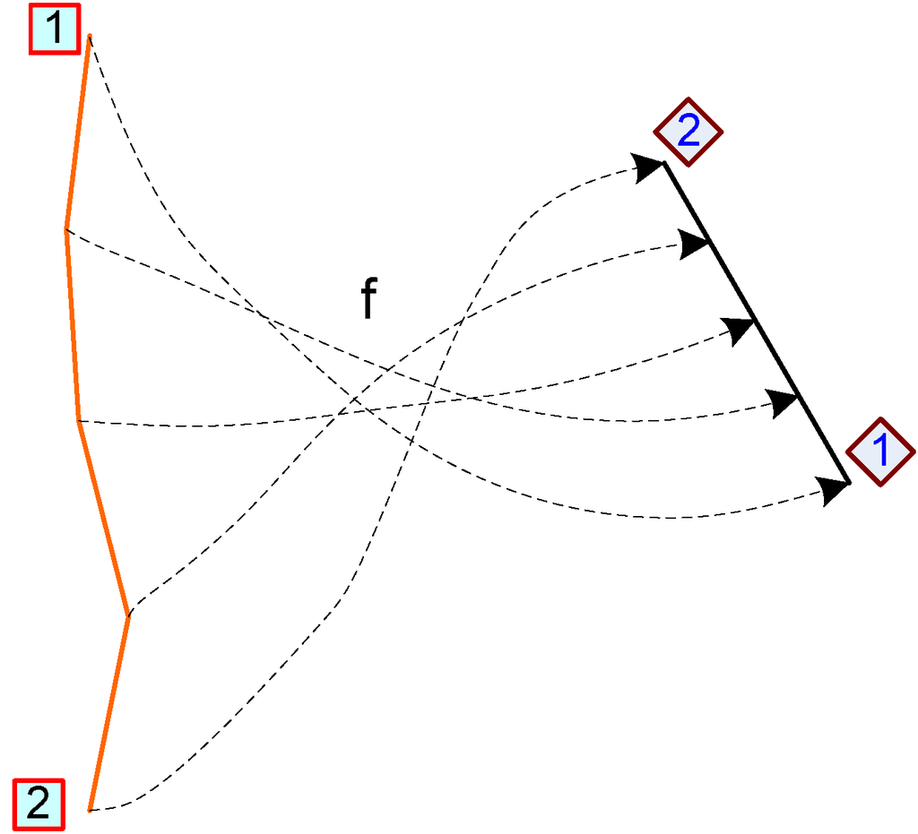
Figure 5.
An example of the “chord” length method.
Figure 5.
An example of the “chord” length method.
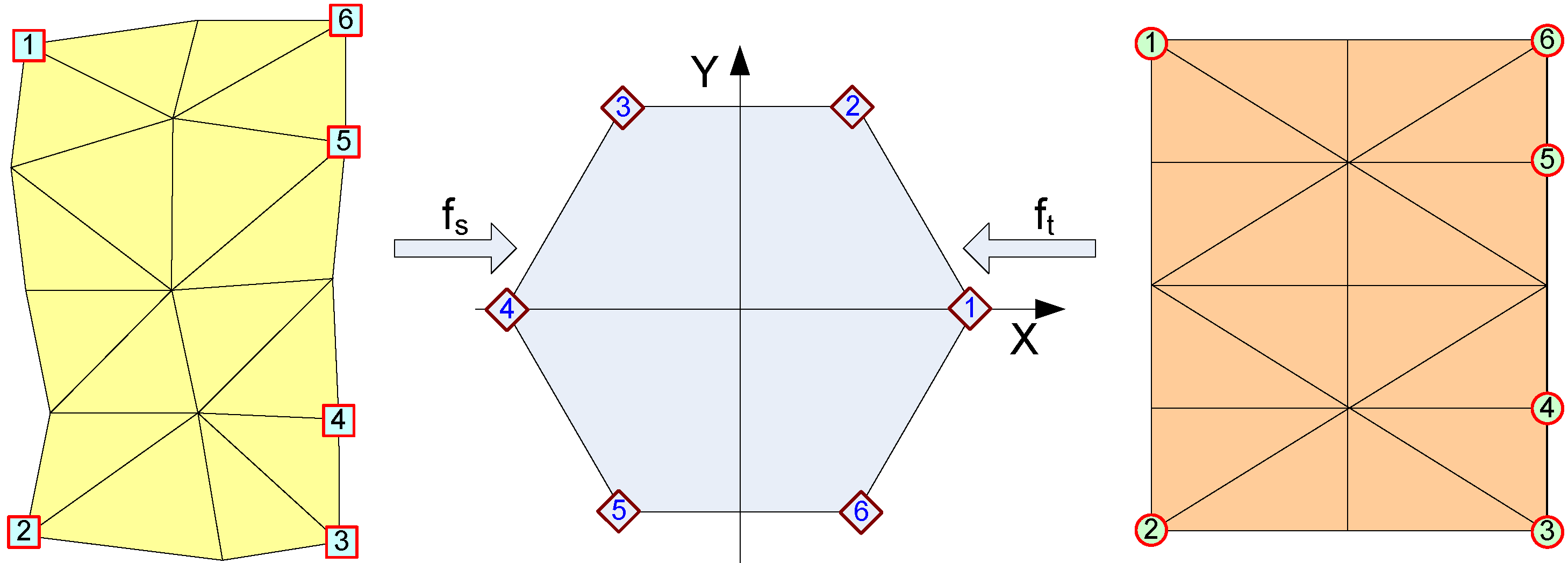
Subsequently, we use mean value parameterization [7,9] to obtain bijective maps, fs and ft, from Ls and Lt, respectively, to this unit regular k-polygon. The composition map, f = ft−1 × fs, is a bijection from Ls to Lt. Figure 6 displays an example of these parameterizations.
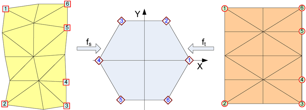
Figure 6.
Parameterizations to the unit regular k-polygon.
Figure 6.
Parameterizations to the unit regular k-polygon.
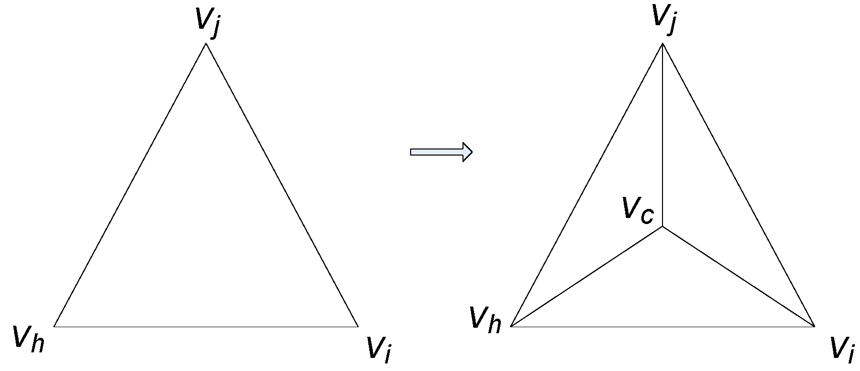
In the second step, we construct a new mesh, Lst, by a set of its vertices, which is an image of V through f, U = f(V), and the topology, T, of Ls, i.e., Lst(U,T). Note that Lst is a compatible mesh of Ls; all of its vertices are on Lt, and it is an approximate mesh of Lt. We require that Lst is a “good” approximation of Lt, i.e., the error between Lst and Lt is smaller than the user’s threshold. Because all of the vertices of Lst are on Lt, the distance from every vertex of Lst to Lt is zero. Therefore, the error between Lst and Lt is the maximum of the distances from the interior vertices of Lt to Lst, as shown in the definition of terms. To obtain a smaller error than the user’s threshold, we complete the following procedures. For each interior vertex, wi, of the target mesh, Lt(W,F), if the distance, di, from wi to the mesh, Lst(U,T), is greater than the user’s threshold, ɛ, and the triangle (vi,vj,vh) contains a point, p, where ||wi,p||=di, we subdivide a triangle (vi,vj,vh) into three triangles by inserting a new point at its centroid and updating Ls (clearly, the error between the old Ls and the updated Ls is zero, so for clarity, we still denote the updated mesh by Ls(V,T)). Figure 7 presents an example of this subdivision. If such a modification has been completed, then the new mesh, Lst, would need to be constructed and checked for error again. Notice that this subdivision reduces the error between Lt and Lst and does not affect other patches.
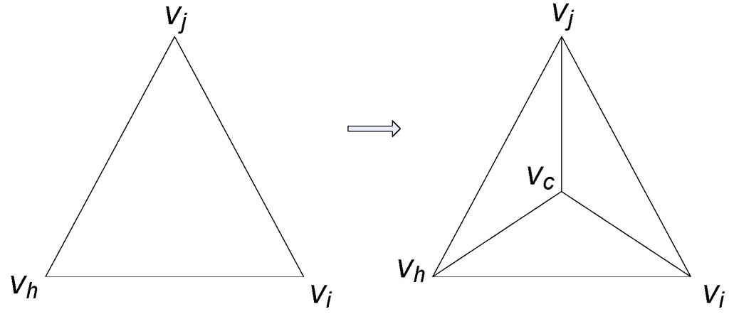
Figure 7.
Splitting a triangle (vi,vj,vh) into three new triangles, (vi,vj,vc), (vj,vh,vc), (vh,vi,vc), by inserting a new point, vc, at the centroid of triangle (vi,vj,vh).
Figure 7.
Splitting a triangle (vi,vj,vh) into three new triangles, (vi,vj,vc), (vj,vh,vc), (vh,vi,vc), by inserting a new point, vc, at the centroid of triangle (vi,vj,vh).
After the above two steps, Ls(V,T) and Lst(U,T) are compatible meshes, and the error between Lst and Lt is smaller than the threshold, ɛ. This mesh pair can be represented by the mesh, Ls(V,T), and a sequence of displacement vectors, where each displacement vector is the difference of a vertex, u, in U and its corresponding vertex, v, in V.
3.6. Finding Trajectories
This sub-procedure is used to find paths in which vertices of the source mesh evolve into their corresponding target vertices. In the case of no attaching constraints, i.e., the source mesh is free to evolve from its original shape into its target shape, trajectories of all its vertices are defined by their linear trajectories (the first and the second experiments in Section 4), and the rest of this calculation can be ignored. When some attaching constraints are used to constrain the geometry of the source mesh during its evolution, trajectories of vertices need to be calculated from their linear trajectories (the third experiment in Section 4). Trajectories of vertices, which impose 1 or 2-controlling surface attaching constraints, are projected lines of their linear trajectories to the controlling surface or the intersection line of the two controlling surfaces, respectively. Trajectories of boundary vertices without attaching constraints are their linear trajectories. Trajectories of all interior vertices are calculated by solving spare linear systems of equations. The algorithm is described as follows.
Given a triangle mesh, Ls(V,T), where V = (v1, v2, …, vn) is a sequence of n vertices, let m, the number of vertices of each trajectories, be a user-defined integer, m ≥ 2. By using attaching constraints, the vertices set, V, of Ls can be subdivided into disjoint subsets:
 where VI is the set of interior vertices, VB0 is the set of boundary vertices without attaching constraints, VB1 is the set of boundary vertices with 1-controlling surface attaching constraints and VB2 is the set of boundary vertices with 2-controlling surface attaching constraints.
First, trajectories of vertices in VB0, VB1 and VB2 are initialized by connecting the vertices of VB0, VB1 and VB2 to their corresponding vertices to create line segments. Then, we subdivide these line segments into m − 1 equal length sub-segments, i.e., linear trajectories are constructed for each boundary. Subsequently, trajectories of vertices in VB1 are modified by replacing their vertices with their projection into controlling surfaces; the trajectory of each vertex in VB2 is modified by changing its vertices to its projection into the curve, which is the intersection of the two controlling surfaces of the vertex.
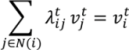
We calculate trajectories of vertices in VI by calculating m − 2 intermediate meshes when the mesh, Ls(V,T), evolves into its corresponding mesh, Lst(U,T). We label Ls with L1, Lst with Lm and intermediate meshes with Lt for each t = 2, …, m − 1. The boundary of the mesh, Lt, is defined by trajectories of vertices in VB0, VB1 and VB2. We also assume that each interior vertex of Lt is a convex combination of its neighbors as follows. Let N(i) be the set of vertex indices of the neighborhood of vertex  , and let II be the index set of VI. A set of non-negative real values,
  , exists, such that:
 and Equation (1) below is satisfied for all i in II:
, and let II be the index set of VI. A set of non-negative real values, , exists, such that:
We calculate  based on the values,
  and
and  , from the first mesh and the last mesh, L1, Lm, as in Equation (2):
based on the values, and , from the first mesh and the last mesh, L1, Lm, as in Equation (2):
Values and are calculated from L1 and Lm using the mean value as described in [7] with Equation (3) and notations in Figure 8.
and are calculated from L1 and Lm using the mean value as described in [7] with Equation (3) and notations in Figure 8. 
Because 0 ≤ αj−1, αj ≤ π, λij in Equation (3) is defined and non-negative, in Equation (2) is non-negative for each t = 2, …, m − 1. Equation (1) gives a sparse linear system of equations, which can be solved sufficiently by a solver, such as OpenNL [20] or Eigen [21]. This system of equations has a unique solution, provided in [8,9]. Because of the unique solution, all trajectories of L have been defined.
in Equation (2) is non-negative for each t = 2, …, m − 1. Equation (1) gives a sparse linear system of equations, which can be solved sufficiently by a solver, such as OpenNL [20] or Eigen [21]. This system of equations has a unique solution, provided in [8,9]. Because of the unique solution, all trajectories of L have been defined.
Figure 8.
Angle notations.
Figure 8.
Angle notations.
Note that by using mesh representations where the topology is explicitly stored, determining the neighborhood, N(i), of vertex vi is trivial. Such mesh representations include G-Maps, C-Maps, Cell-Tuple-Structure, Halfedge data structure, etc.
4. Software and Experiments
The algorithm described in Section 3 has been implemented as a gOcad plug-in. This software uses Boost C++ libraries [22] and the Computational Geometry Algorithms Library (CGAL) [23]. To use CGAL parameterization when the parameterization domain is a unit regular k-polygon, a new class implementing the BorderParameterizer_3 concept has been implemented. In this software, we used the OpenNL library [20], integrated with CGAL, as a solver for sparse linear equations to find trajectories. The software provides a graphical user interface for the end-user to input and modify the constraints. The boost graph library is used to find the shortest path to construct cutting and fence paths.
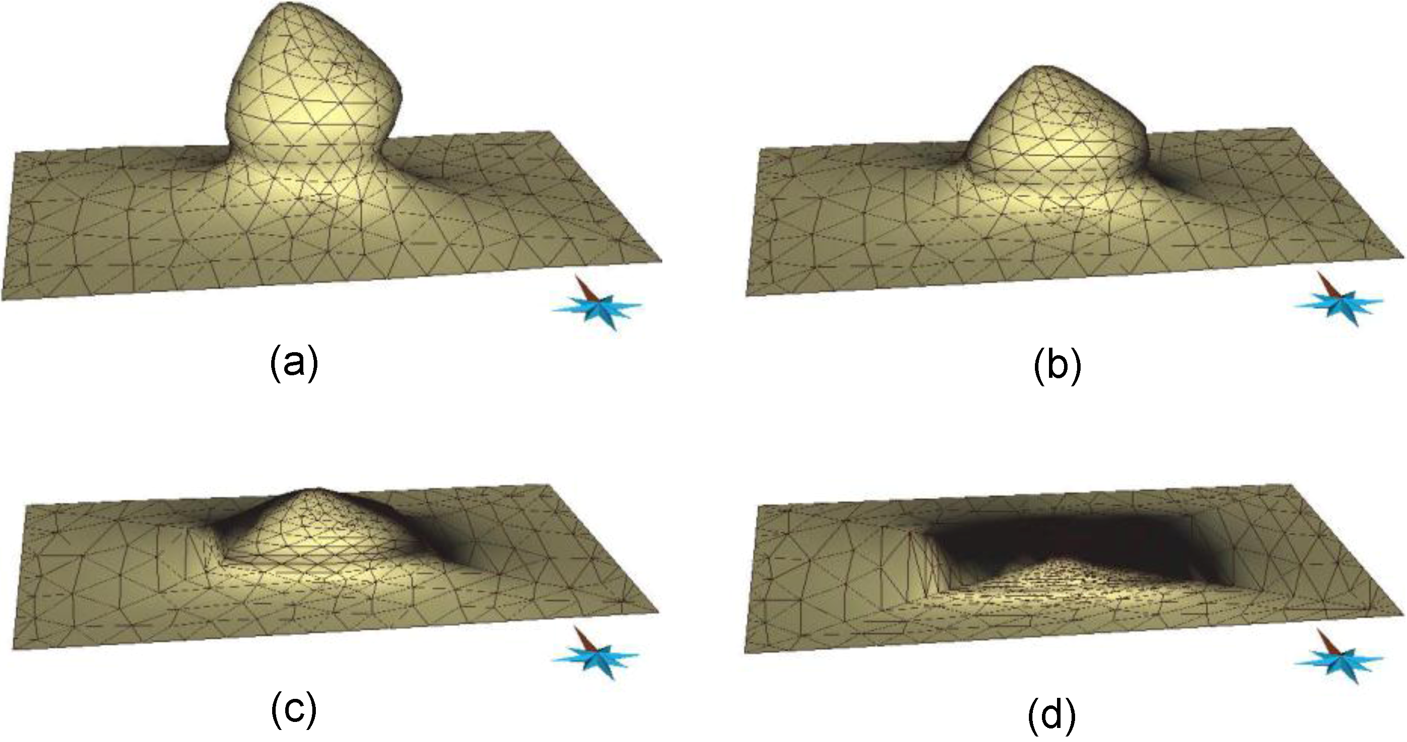
The software was tested with three sample data sets. The first was the salt dome data, and the second and third were fictitious data for faulting, deposition and erosion processes. In the first experiment, we constructed data for a salt dome given by its current shape and its previous shape as a flat surface. The constraints needed for this experiment were four pairs of control vertices. Figure 9 displays some snapshots of the salt dome.

Figure 9.
A salt dome in time. (a) t = 1, (b) t = 2/3, (c) t = 1/2, (d) t = 0.
Figure 9.
A salt dome in time. (a) t = 1, (b) t = 2/3, (c) t = 1/2, (d) t = 0.
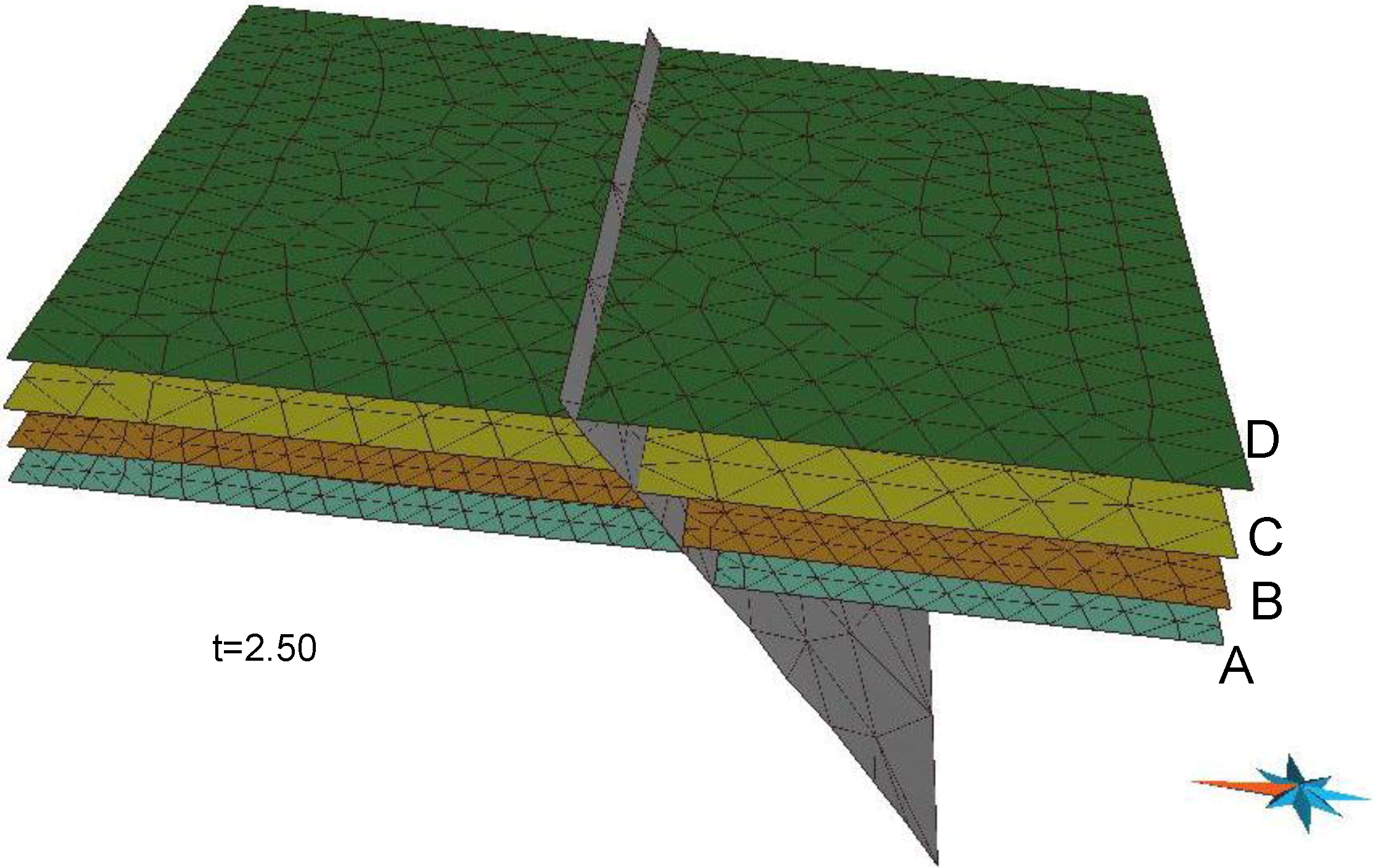
In the second experiment, the given data included four sets of data at four time instances, t = 1, t = 2, t = 3 and t = 4. At time t = 4, there were six surfaces, namely five geological horizons, A, B, C, D and E, and the fault (Figure 10a). At time t = 3, five surfaces represented four geological horizons, A, B, C and D, and the fault (Figure 10b). At time t = 2, the given data included four surfaces, A, B and C, and the fault (Figure 10c). At time t = 1, three surfaces represented two geological horizons A and B, and the fault (Figure 10d). The fault was assumed constant throughout the entire time interval [1, 4], and the geological horizon, E was constant in the interval [3, 4]. Each horizon in each time interval was run using the software. For example, to construct spatio-temporal data of the geological horizon, B, in time interval [2, 3] from two of its shapes at time instances t = 2, 3, we only had to set up eight pairs of control vertices. Figure 11 shows the geological horizon, B, in time interval [2, 3]. By putting all of the results of the constructed data of each horizon in each time interval in the same space and time coordinates, we simulate geological processes in an area and in a specific time interval. Figure 12 shows the geological structure in the area of interest at time t = 2.50.

Figure 10.
Given data at time instances. (a) t = 4, (b) t = 3, (c) t = 2, (d) t = 1.
Figure 10.
Given data at time instances. (a) t = 4, (b) t = 3, (c) t = 2, (d) t = 1.
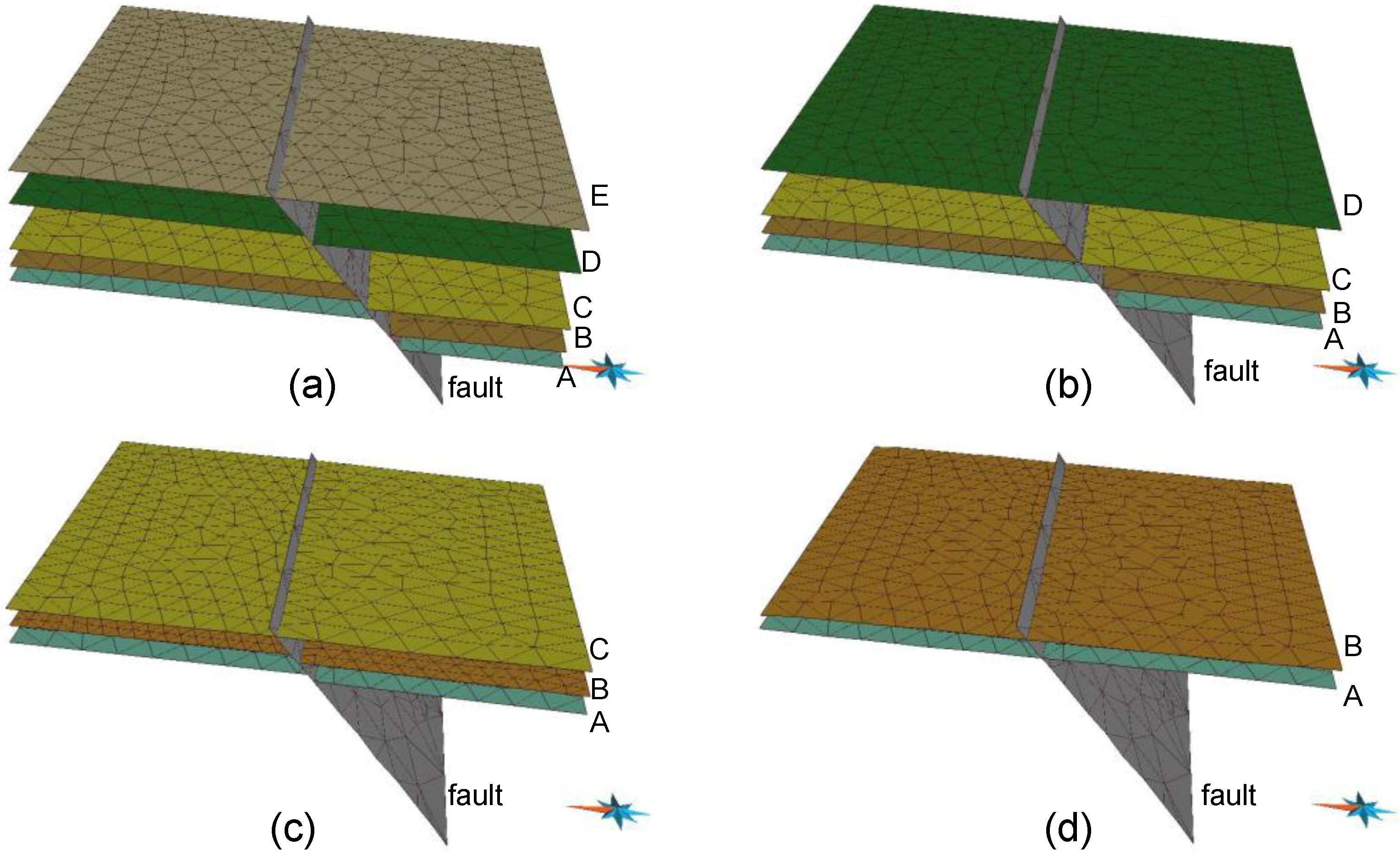

Figure 11.
The geological horizon, B, in time interval [2, 3].
Figure 11.
The geological horizon, B, in time interval [2, 3].
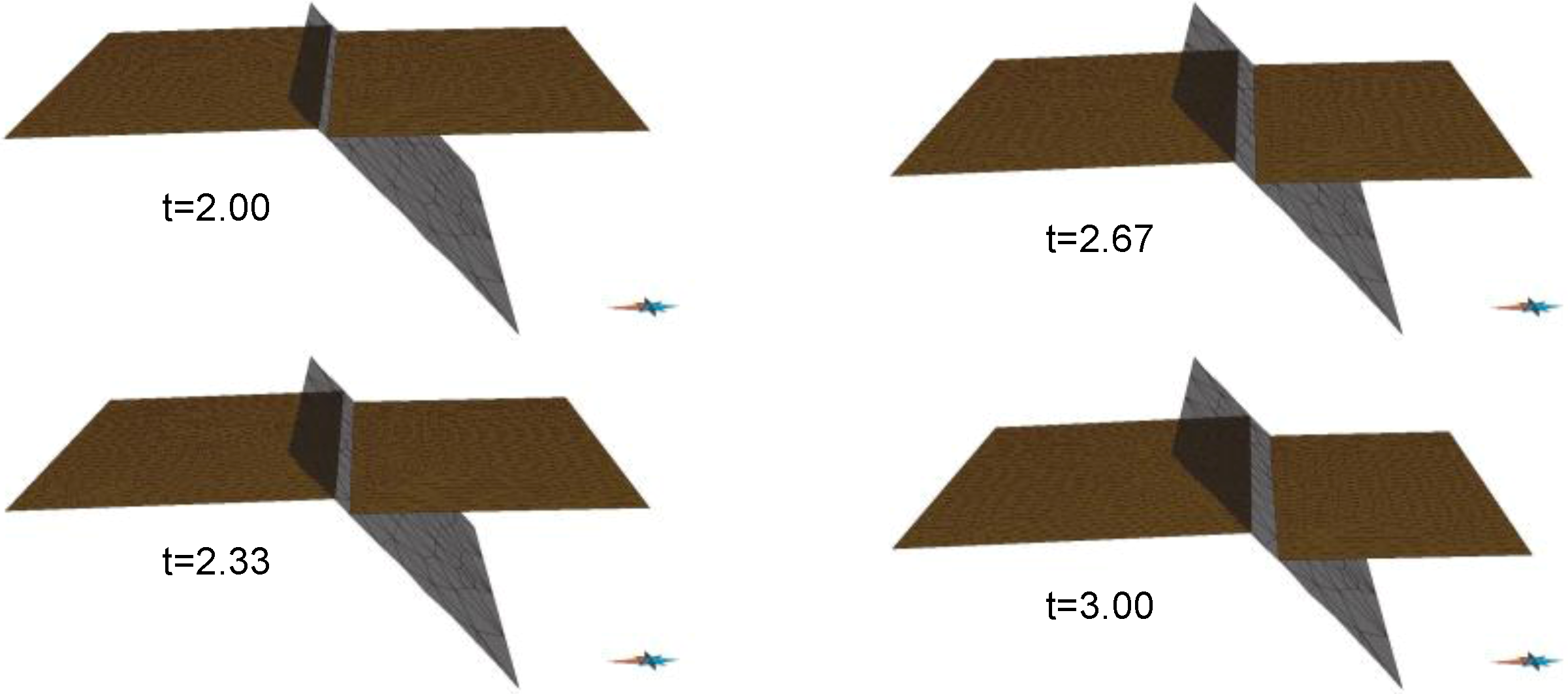

Figure 12.
The geological structure of an area of interest at time t = 2.50.
Figure 12.
The geological structure of an area of interest at time t = 2.50.
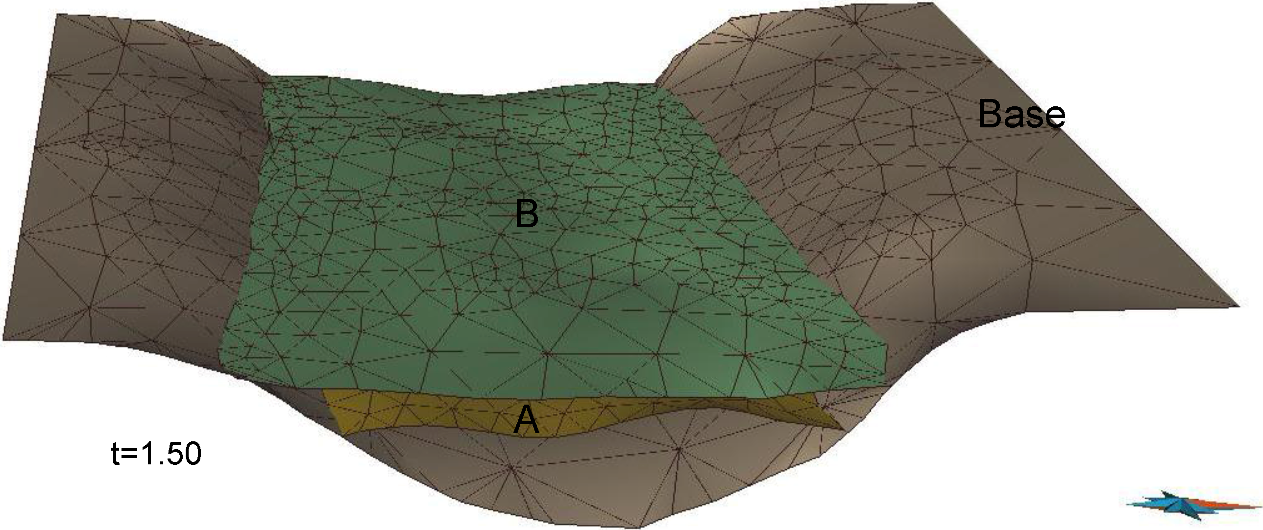
In the third experiment, we worked with four surfaces, namely, a basement surface and top surfaces, A, B and C, of sediments A, B and C, respectively. Data were given at six time instances: t = 5 (Figure 13a), t = 4 (Figure 13b), t = 3 (Figure 13c), t = 2 (Figure 13d), t = 1 (Figure 13e) and t = 0 (Figure 13f). The basement surface was assumed constant. We constructed the data of surfaces in time interval [0, 5] by constructing the data of each surface (A, B, C) in each time interval, [0, 1], [1, 2], [3, 4] and [4, 5]. For the purpose of brevity, we only describe the procedure to construct data of surface B in time interval [1, 2]. In this case, the source mesh was surface B at time t = 2, and the target mesh was surface A at time t = 1. The controlling surface was the basement surface. Attaching constraints were used to keep surface B in constant contact with the basement surface. Unlike the first and the second experiments, in which linear trajectories were used, trajectories had to be calculated using the finding trajectories sub-procedure, as shown in Subsection 3.4. Figure 14 shows the data of surface B in time interval [1, 2]. After constructing all of the data, the final data were put in the same space and time coordinates to simulate geological processes—sedimentation and erosion, in this case. Figure 15 depicts the geological structure in the area of interest at time t = 1.50.

Figure 13.
Given data at six time instances. (a) t = 5, (b) t = 4, (c) t = 3, (d) t = 2, (e) t = 1, (f) t = 0.
Figure 13.
Given data at six time instances. (a) t = 5, (b) t = 4, (c) t = 3, (d) t = 2, (e) t = 1, (f) t = 0.
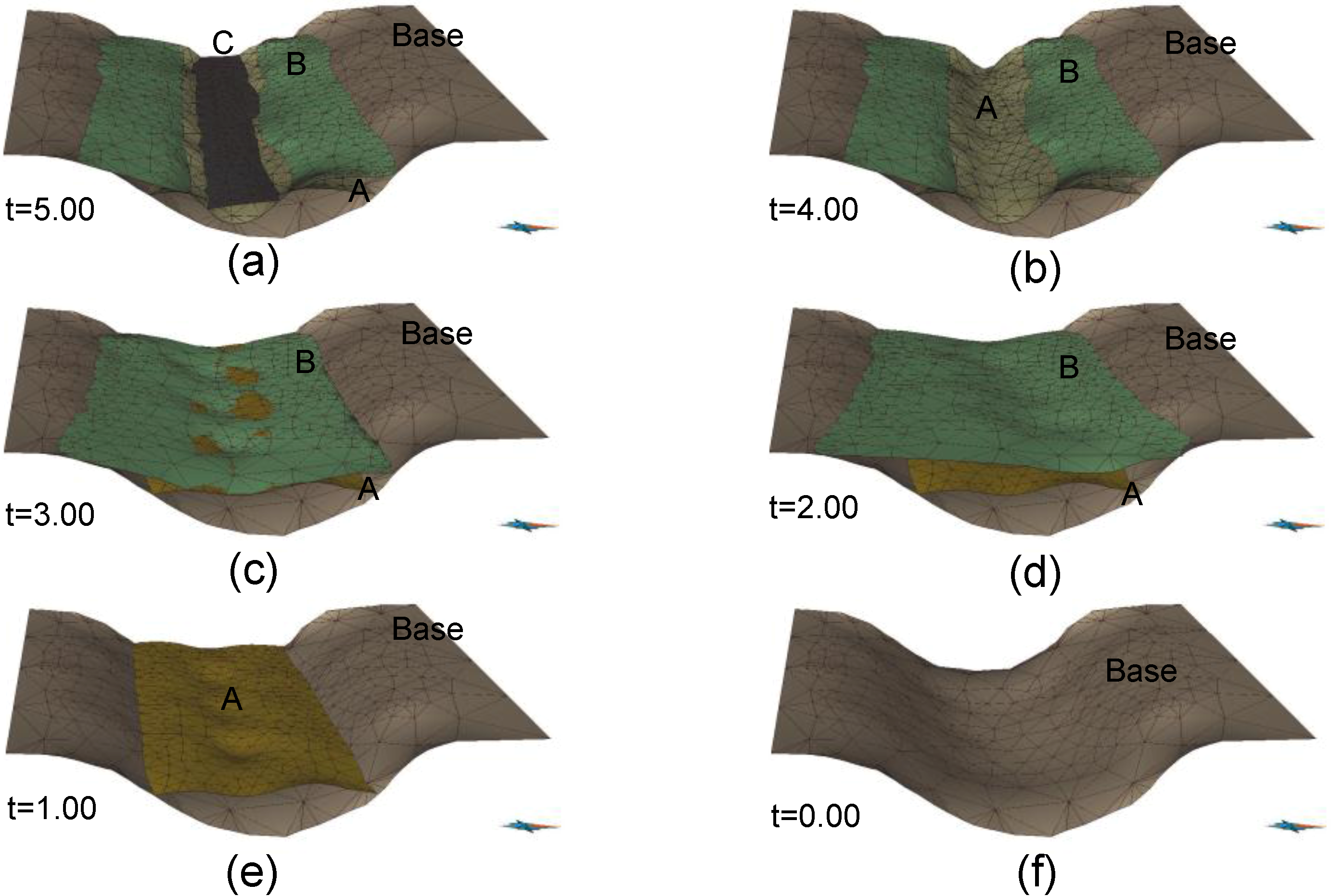
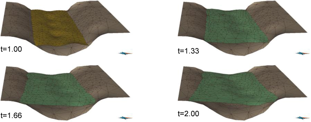
Figure 14.
Top surface B in time interval [1, 2].
Figure 14.
Top surface B in time interval [1, 2].


Figure 15.
The geological structure of an area of interest at time t = 1.5.
Figure 15.
The geological structure of an area of interest at time t = 1.5.
5. Discussion and Conclusions
Our method has shown its efficiency and effectiveness for a rough construction of spatio-temporal data with constraints in terms of geometry (without physical and mechanical constraints). It is useful when no physical or mechanical process models are available or when there are not sufficient data for these models. Our method consists of four main procedures in which the first two procedures are semi-manual and the last two procedures are automatic. Our contributions include a new cutting procedure and a new sub-procedure for finding trajectories using convex combinations. Due to the cutting procedure, our method can work with arbitrary meshes. By partitioning meshes into patches, i.e., triangle meshes homeomorphic to disks, the method reduces the original problem to smaller and simpler problems. Obviously, we can obtain more advantageous results through parallel computing methods. The main calculations include calculating the parameterization sub-procedure and the finding trajectories sub-procedure; the complexities of both are equal to the complexity of a convex, fixed-boundary parameterization method, e.g., the mean value parameterization method. Timings of some parameterization algorithms are presented in [11].
In summary, we emphasize the achieved results in this study as follows:
- (1)
- Introduction of a new method for construction of spatio-temporal data in the geosciences.
- (2)
- Implementation of the algorithm as a gOcad plug-in.
- (3)
- Experimentation with some samples.
In the future, our work will aim to improve the algorithm for the finding trajectory sub-procedure and developing a new algorithm for objects other than triangle meshes, such as solids or objects in higher dimensions.
Acknowledgments
We would like to express our sincere thanks to Helmut Schaeben, Jan Gietzel and Paul Gabriel for their help and advice. Many thanks to Ines Görz for her suggestion and careful preparation of the sample data in Section 4. Special thanks to Chi Ngoc Le, Ramadan Abdelaziz and Minh Phuong Kieu for their language correction. Finally, we also would like to thank the anonymous reviewers and the editors for their comments and suggestions on the manuscript.
Conflicts of Interest
The author declares no conflict of interest.
References
- Le, H.H.; Gabriel, P.; Gietzel, J.; Schaeben, H. An object-relational spatio-temporal geoscience data model. Comput. Geosci. 2013, 57, 104–115. [Google Scholar] [CrossRef]
- Iwanowski, M.; Serra, J. Morphological Interpolation and Color Images. In Proceedings of the 10th International Conference on Image Analysis and Processing ICIAP’99, Venice, Italy, 27–29 September 1999; IEEE Computer Society: Washington, DC, USA, 1999; pp. 50–55. [Google Scholar]
- Sirakov, N.M.; Granado, I.; Muge, F.H. Interpolation approach for 3D smooth reconstruction of subsurface objects. Comput. Geosci. 2002, 28, 877–885. [Google Scholar] [CrossRef]
- Mouravliansky, N.; Matsopoulos, G.K.; Delibasis, K.; Asvestas, P.; Nikita, K.S. Combining a morphological interpolation approach with a surface reconstruction method for the 3-D representation of tomographic data. J. Vis. Commun. Image R. 2004, 15, 565–579. [Google Scholar] [CrossRef]
- Kels, S.; Dyn, N. Reconstruction of 3D objects from 2D cross-sections with the 4-point subdivision scheme adapted to sets. Comput. Graph. 2011, 35, 741–746. [Google Scholar] [CrossRef]
- Floater, M.S.; Gotsman, C. How to morph tilings injectively. J. Comput. Appl. Math. 1999, 101, 117–129. [Google Scholar] [CrossRef]
- Floater, M.S. Mean value coordinates. Comput. Aided Geom. Des. 2003, 20, 19–27. [Google Scholar] [CrossRef]
- Floater, M.S. Parametric tilings and scattered data approximation. Int. J. Shape Model. 1998, 4, 165–182. [Google Scholar] [CrossRef]
- Floater, M.S. Parametrization and smooth approximation of surface triangulations. Comput. Aided Geom. Des. 1997, 14, 231–250. [Google Scholar] [CrossRef]
- Botsch, M.; Kobbelt, L.; Pauly, M.; Alliez, P.; Lévy, B. Polygon Mesh Processing; A K Peters, Ltd.: Natick, MA, USA, 2010; pp. 1–230. [Google Scholar]
- Hormann, K.; Polthier, K.; Sheffer, A. Mesh Parameterization: Theory and Practice. In SIGGRAPH Asia 2008 Course Notes; ACM Press: Singapore, 2008; pp. 1–87. [Google Scholar]
- Lipman, Y.; Levin, D.; Cohen-Or, D. Green coordinates. ACM Trans. Graph. 2008, 27, 1–10. [Google Scholar] [CrossRef]
- Li, X.; Gu, X.; Qin, H. Surface mapping using consistent pants decomposition. IEEE Trans. Vis. Comput. Graph. 2009, 15, 558–571. [Google Scholar] [CrossRef]
- Liu, Y.S.; Yan, H.B.; Martin, R. As-rigid-as-possible surface morphing. J. Comput. Sci. Technol. 2011, 26, 548–557. [Google Scholar] [CrossRef]
- Yan, H.B.; Hu, S.M.; Martin, R. 3D morphing using strain field interpolation. J. Comput. Sci. Technol. 2007, 22, 147–155. [Google Scholar] [CrossRef]
- Alexa, M.; Cohen-Or, D.; Levin, D. As-Rigid-As-Possible Shape Interpolation. In Proceedings of the 27th Annual Conference on Computer Graphics and Interactive Techniques (SIGGRAPH ’00), New Orleans, LA, USA, 23–28 July 2000; ACM Press: New York, NY, USA, 2000; pp. 157–164. [Google Scholar]
- Van Kaick, O.; Zhang, H.; Hamarneh, G.; Cohen-Or, D. A survey on shape correspondence. Comput. Graph. Forum 2011, 30, 1681–1707. [Google Scholar] [CrossRef]
- Kraevoy, V.; Sheffer, A. Cross-parameterization and compatible remeshing of 3D models. ACM Trans. Graph. 2004, 23, 861–869. [Google Scholar] [CrossRef]
- Praun, E.; Sweldens, W.; Schröder, P. Consistent Mesh Parameterizations. In Proceedings of the 28th Annual Conference on Computer Graphics and Interactive Techniques (SIGGRAPH ’01), Los Angleles, CA, USA, 12–17 August 2001; ACM Press: New York, NY, USA, 2001; pp. 179–184. [Google Scholar]
- OpenNL. Open Numerical Library. Available online: http://alice.loria.fr/index.php/software/4-library/23-opennl.html (accessed on 20 July 2013).
- Eigen. Eigen v3. Available online: http://eigen.tuxfamily.org (accessed on 20 July 2013).
- Boost. Boost C++ Libraries. Available online: http://www.boost.org (accessed on 20 July 2013).
- CGAL. Computational Geometry Algorithms Library. Available online: http://www.cgal.org/ (accessed on 20 July 2013).
© 2013 by the authors; licensee MDPI, Basel, Switzerland. This article is an open access article distributed under the terms and conditions of the Creative Commons Attribution license (http://creativecommons.org/licenses/by/3.0/).