Article

Unveiling Livelihood Vulnerability and Consumption Declines in U.S. Counties During the COVID-19 Pandemic: A Multilevel Analysis

Department of Urban Design and Planning, Hongik University, Seoul 04066, Republic of Korea
*
Author to whom correspondence should be addressed.
ISPRS Int. J. Geo-Inf. 2026, 15(5), 183; https://doi.org/10.3390/ijgi15050183
Submission received: 16 February 2026 / Revised: 20 April 2026 / Accepted: 21 April 2026 / Published: 23 April 2026

Abstract

COVID-19 was a prolonged public-health shock that disrupted mobility, access to services, and household spending. Although the official U.S. poverty rate declined to 11.1%, the Supplemental Poverty Measure rose to 12.9%, suggesting that material hardship persisted unevenly across places. This study asks whether pre-existing livelihood vulnerability and local epidemic burden translated into geographically concentrated consumption losses during 2020–2022. Because sustained consumption loss can erode households’ health-related spending, tracking where spending declines concentrate helps connect local social and environmental conditions to how communities withstand a health crisis. We analyze consumer expenditure, unlike prior research relying on aggregate retail sales, to capture fine-grained economic strains as a proxy for shock-absorption capacity. A Livelihood Vulnerability Index (LVI) was calculated for each U.S. county using 16 socio-economic variables, and counties were classified as high- or low-risk. A multilevel model then examined how socio-economic and COVID-19 factors at county and census tract levels shaped consumption changes. Higher-risk communities experienced greater consumption reductions. At the census tract level, the non-White ratio, vacancy rate, built year, per capita income, education level, and housing value were significant. At the county level, COVID-19 cases and deaths, crowding, public transportation use, and vehicle availability mattered most. These findings support place-targeted strategies that combine public-health response with socio-environmental interventions to reduce disparities rooted in pre-existing vulnerability.

1. Introduction

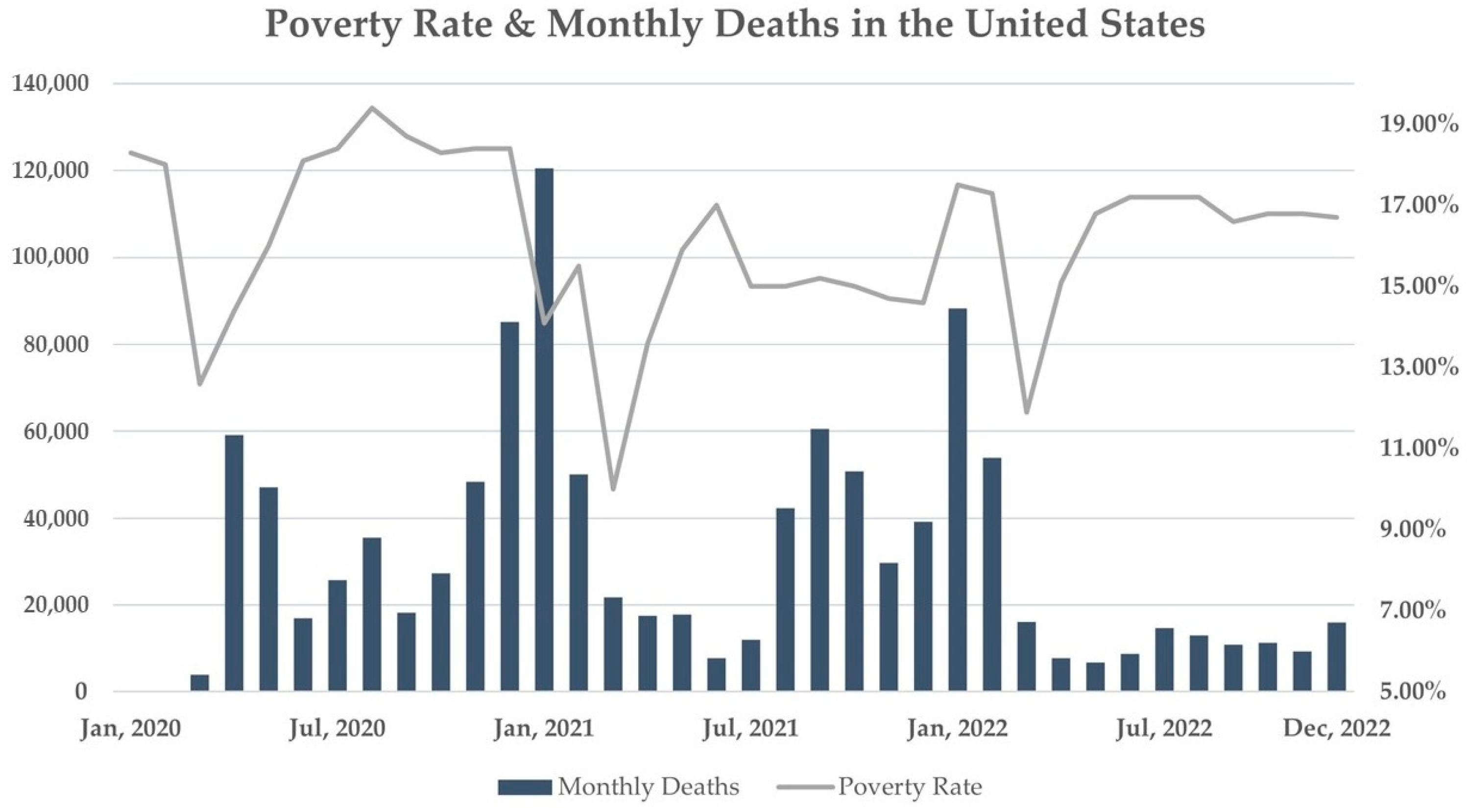
The increasing array of threats confronting cities—natural disasters, socio-economic disparities, and public health crises—has recently elevated the importance of resilience in urban environments [1,2]. However, the concept of resilience has undergone a paradigmatic shift, transitioning from an engineering viewpoint, which prioritizes the rapid restoration of pre-disaster equilibrium, to an ecological viewpoint that highlights the ability to adapt, restructure, and transform in response to stress [3,4]. This distinction is crucial, since a limited emphasis on ‘bouncing back’ frequently neglects systemic socioeconomic disparities, tacitly advocating a reversion to a status quo that was previously detrimental for excluded groups. The COVID-19 pandemic served as a rigorous stress test for this adaptive capacity, revealing how inherent socio-economic disparities exacerbate vulnerabilities during prolonged disruptions (Figure 1) [5,6]. Subsequent empirical analyses, especially those examining compounded risks such as work instability, healthcare access barriers, and consumer volatility, have further exposed critical blind spots in conventional resilience frameworks regarding marginalized populations [5,7,8]. This matters beyond economics alone: when household spending falls, so does the ability to pay for healthcare, adequate food, and other necessities—making the geography of consumption loss a health equity concern as well.
From an ecological resilience viewpoint, a regional system does not merely revert to a singular equilibrium; it could shift among various stable states, potentially becoming trapped in a condition of persistent vulnerability once a critical threshold is crossed [3]. Thus, resilience needs to be understood as a dynamic process of navigating these thresholds rather than a static trait. The COVID-19 pandemic exemplified this dynamic, showing how structural inequalities—such as the residential segregation described by Massey and Denton (1993)—act as preconditions that dictate whether a community adapts or collapses under systemic shock [4,5,9]. While some areas quickly calmed and effectively reduced the consequences of the epidemic, others, especially underprivileged populations marked by past injustices, saw protracted periods of social unrest [6]. Therefore, understanding resilience within regional systems requires realizing these several equilibria and the critical thresholds that start systematic shifts.
Resilience planning has drastically shifted from reactive recovery to the development of adaptive capability by utilizing Holling’s concept. Ecological resilience evaluates performance by balancing results among population subgroups, particularly for marginalized communities living with compounding vulnerabilities, whereas engineering resilience focuses more on efficiency metrics like GDP recovery durations. To better understand these dynamics, the adaptive cycle model posits that systems do not exist in a permanent state of stability but alternate between phases of conservation and reorganization [10]. Using this framework to the current study, the COVID-19 pandemic represents a ‘release’ phase, where structural tightness is broken, and accumulated resources are dispersed. In this context, identifying regional adaptation thresholds requires analyzing ‘slow variables’—such as housing stock aging and labor market structure—rather than just immediate shocks. By continuously monitoring these gradual shifts, it becomes possible to spot crucial turning points before a systemic collapse occurs [11]. This perspective is essential for sustainable regional growth because it helps clarify how the system may reorganize into a new configuration after an external shock [3,12].
The social and economic resilience of cities was put to the test in earnest by the COVID-19 pandemic. Significant changes in economic activity and consumption patterns were brought about by this crisis, which had an unprecedented quality and highlighted the weaknesses and disparities inherent in the current social system [13]. The pandemic did not simply generate new dangers; it made existing vulnerabilities worse, especially for low-income households, ethnic minorities, and the elderly who were already navigating insufficient economic conditions. These groups faced compounded challenges, where low-paying, unstable jobs converged with poor housing and limited healthcare. Therefore, assessing this vulnerability—specifically how it translates into tangible economic decline—has become a prerequisite for effective policy response in urban planning. To address this need, this study aims to analyze the direct relationship between livelihood vulnerability and the volatility of individual consumption expenditure.
This study examines how pre-existing livelihood vulnerability and local pandemic conditions were associated with changes in consumer expenditure across U.S. counties and census tracts during the COVID-19 pandemic. A Livelihood Vulnerability Index was constructed to classify counties by vulnerability status, and a multilevel model was then estimated using the percentage change in consumer expenditure between 2020 and 2022 as the dependent variable. This approach allows us to separate local neighborhood conditions from broader county level pandemic and mobility contexts while assessing how these factors relate to disparate expenditure outcomes. Instead of proposing a universal alternative to existing vulnerability indices, the study applies a livelihood-oriented classification framework to examine whether pre-existing socio-economic and built-environment vulnerability was associated with differential expenditure loss during a prolonged public-health shock. By focusing on expenditure change rather than aggregate retail recovery alone, the analysis captures a more direct, household-level measure of economic strain. The next section reviews key concepts and empirical studies on urban resilience, vulnerability, and consumption dynamics during crises, setting the stage for the specific gap addressed in this study.

2. Literature Review

2.1. Resilience

Resilience theory has transitioned from an engineering perspective—focused on rapid infrastructure recovery—toward an ecological paradigm that emphasizes a system’s dynamic adaptation and equitable reorganization after a shock [3,4,14]. In urban economics, this adaptive capacity becomes apparent through interacting governance networks, material flows, and socio-economic dynamics [15,16,17].
Recent studies emphasize the role of consumption patterns as proxies for resilience, aligning with this research’s focus on expenditure volatility. Traditional metrics relying on aggregate retail sales often mask disparities, as seen in the divergent recovery rates of high-income versus low-income ZIP codes [5]. For example, although national retail spending recovered to pre-pandemic levels by late 2021, areas with high vacancy rates and aged housing stock had noticeably slower recovery paths, therefore showing ingrained built environment vulnerabilities. These spatial differences complement our research on how housing features—such as vacancy rates and building age—mediate consumption resilience at the census tract level, so highlighting the part preexisting infrastructure inequalities play in determining post-crisis economic outcomes [9].
One important breakthrough has been the inclusion of vulnerability assessments into resilience building. Building on this framework, our Livelihood Vulnerability Index (LVI) approach identifies communities where economic solutions must solve structural inequalities (e.g., racialized credit access) as well as urgent shocks (e.g., job loss), hence bridging resilience and vulnerability. Such approaches challenge the artificial divide between resilience as “recovery” and vulnerability as “risk”, instead framing them as interdependent dimensions of urban systems.

2.2. Vulnerability

When pre-existing vulnerabilities persist, the constraints of resilience strategies become abundantly clear. Originally conducted in natural hazard research, vulnerability studies evolved to solve structural inequalities ingrained in metropolitan environments. Ref. [18] tripartite framework—exposure, sensitivity, and adaptive capacity—offers a prism through which to view how past events magnify crisis effects. Racial-divided communities in the United States experienced mortality rates higher than those in mostly White areas during COVID-19, a difference driven by healthcare deserts and overcrowded housing [19,20]. These structural weaknesses set off a chain reaction of economic consequences, and medical debt disproportionately taxed household budgets in underdeveloped areas.
Redlining and other past policies throw lengthy shadows over modern vulnerability. Massey and Denton’s (1989) hypersegregation framework helps explain how historic residential segregation patterns intensified socio-economic vulnerabilities during the COVID-19 pandemic, particularly in previously redlined neighborhoods [21]. Housing stock features also mediated outcomes: communities with high-density multifamily apartments, such as Los Angeles’s Koreatown, had far higher infection rates than suburban single-family areas, therefore aggravating consumption reductions through health-related financial shocks.
The epidemic exposed, even more, how systematic weaknesses reinterpret consumer preferences depending on limited capacities. Longitudinal studies during the COVID-19 pandemic revealed that individuals with chronic medical conditions faced significant trade-offs in healthcare utilization. Specifically, adults and children with atopic dermatitis delayed necessary medical treatments at a rate 1.89 times higher than unaffected populations, with 32.7% reporting postponed care to minimize exposure risks [22]. During the COVID-19 pandemic, delayed prescription refills contributed to significant medication nonadherence, disproportionately affecting low-income households who rely on public transit for pharmacy access [23,24]. These behavioral changes fit Sen’s (1999) capability framework, which views health decisions not as autonomous choices but rather as negotiations within the structured agency, where systematic barriers like healthcare deserts and digital divides limit individuals’ freedom to achieve valued functions [25,26].
Pandemic-related service disruptions created additional barriers for vulnerable populations, including delayed or forgone care and increased affordability burdens [22,23]. Such denial of conversion factors exacerbated already existing inequalities as marginalized groups suffered compounding losses in health, economic stability, and social involvement [26,27].
Policy responses must address these overlapping vulnerabilities. Despite growing evidence on targeted intervention, current studies still do not fully explain how built-environment inequalities such as aging infrastructure and housing vacancies shape local economic resilience during crises [28].

2.3. Research Gap

Existing social vulnerability indices effectively identify demographic risks but rarely connect built-environment vulnerabilities to households’ direct economic resilience during prolonged disruptions. Methodologically, while existing resilience studies typically evaluate post-crisis recovery through macro-level economic indicators (e.g., aggregate retail sales, GDP) this approach suffers from a critical theoretical blind spot. Retail sales reflect the volume of business transactions at the point of sale; thus, the metric can artificially inflate if a neighborhood attracts a temporary influx of external visitors or undergoes commercial gentrification, masking the acute economic strain experienced by actual residents. For instance, a tourist-heavy district might show a rapid retail recovery that falsely signals resilience, while the local residential population continues to suffer from severe financial hardship.
To address this gap, this study demonstrates clear novelty by introducing consumer expenditure as the primary outcome variable. Because this metric is aggregated based on the point of residence rather than the point of sale, it systematically excludes the distortion caused by external consumer influx. While it remains a tract level aggregate, it serves as a more reliable proxy for the collective shock-absorption capacity of the local population. The empirical advantage of this residence-based approach is that it prevents a spatial ecological fallacy; while retail sales might falsely signal local recovery due to commercial gentrification, consumer expenditure provides an empirically robust baseline to accurately target relief funds toward actual populations experiencing livelihood contraction. By shifting the analytical focus from commercial spatial recovery to residential consumption maintenance, this study reveals the precise socio-spatial mechanisms driving unequal economic resilience.

3. Materials & Methods

3.1. Variables (Table 1)

The consumer expenditure data included in this study are sourced from Market Profile Data, which systematically amalgamates demographic, economic, housing, and consumer behavior indicators from diverse governmental and market research entities. Consumer expenditure data are derived from the most recent Consumer Expenditure Survey (CEX) administered by the Bureau of Labor Statistics (BLS). The CEX consists of two elements: a diary survey that collects comprehensive weekly expenditure data over two successive weeks and a quarterly rotating interview survey involving around 5000 consumer units, which addresses spending on significant or frequently purchased items such as real estate, automobiles, and major appliances. The interview survey constitutes almost 95% of the overall reported expenditure. A “consumer unit” is described as a household consisting of individuals linked by blood, marriage, adoption, legal arrangement, solitary individuals, or groups collectively responsible for significant expenses. The survey records expenditures encompassing the complete transaction costs of goods and services, including relevant sales taxes, which the BLS uses to revise the market basket for the calculation of the Consumer Price Index (CPI).
To examine the impact of socio-economic vulnerability on consumption changes during the COVID-19 epidemic, we selected a set of demographics, economic, and infrastructure factors at two spatial levels. While Level 2 variables (county) reflect a larger context, including migration factors and pandemic severity, Level 1 variables (census tract) capture local population and housing features. Based on past vulnerability and resilience studies [29,30], these variables—which include elements like minority status, transit access, and crowding—were selected, reflecting themes stressed in the CDC’s Social Vulnerability Index. Table 1 lists every variable together with its definition, measuring scale, and data source. Consistent with results showing that under crisis conditions, disadvantaged communities suffer more severe economic impacts, our analysis indicates that census tracts and counties with higher social and infrastructure vulnerabilities (e.g., greater minority population, lower income, higher crowding) will show greater declines in consumer expenditure.
Table 1. Characteristics of variables used in the study analyses.
DomainVariableDescriptionSource (Year)Key References
Variables
(Socio-economic Status)
Level 1
Census Tract
Non-WhitePercentage of residents recorded in ACS categories other than non-Hispanic White alone, including Hispanic or Latino residents.U.S. Census Bureau
ACS (5-year estimates)
2020–2022
[31,32].
VacancyPercentage of vacant structures.[33,34]
Average building yearAverage construction year of residential buildings.[31,35].
Per capita incomeMean income per person in the census tract (U.S. dollars).[36,37].
EducationPercentage of residents without a high school diploma.[38,39].
EmploymentPercentage of workers employed in secondary industries (manufacturing, construction, etc.) relative to total workforce.[39,40].
Housing ValueMedian value of owner-occupied housing units (U.S. dollars).[41,42].
Level 2
County
CrowdingPercentage of households with more than one person per room.[43,44].
Public TransportationPercentage of workers commuting via public transit.[45,46].
Commute TimePercentage of workers with daily commutes exceeding 30 min.[45,47].
Households without a vehiclePercentage of households without access to a vehicle.[48,49].
Population DensityNumber of people per square mile in a given area.[50,51].
Confirmed cases of COVID-19Confirmed COVID-19 cases per 100,000 population.CDC COVID Data
Tracker (2020–2022)
[52,53].
Death cases of COVID-19COVID-19-related deaths per 100,000 population.[52,53].
Definitions, units, and data sources for variables used in the multilevel analysis of consumption changes. Level 1 (census tract) variables measure local demographic, economic, and housing conditions, whereas Level 2 (county) variables capture broader housing, mobility, density, and pandemic conditions. Percentage-based variables are expressed as percentages (%); COVID-19 cases and deaths are reported per 100,000 population; population density is measured as persons per square mile; and income and housing value are expressed in U.S. dollars.
The census tract variables within neighborhoods reflect aspects of social and economic vulnerability. Higher non-White population share, for instance, is typically linked with historical and structural disadvantages; places with larger racial/ethnic minorities faced proportionally higher COVID incidence and economic disruption.
Lower per capita income, lower educational attainment, and more secondary-industry employment point to economic disadvantages and job precarity; that is, a lack of household capacity to withstand crises. Similarly, housing value and vacancy rates reflect wealth and physical infrastructure: communities with older, lower-value homes or high vacancy generally see ongoing disinvestment, hence aggravating vulnerability. Research on urban decline reveals that areas of concentrated disadvantage usually match high vacancy and aging building stock (the prevalence of prosperous, shrinking cities). The census tract level features in our model function as controls for neighborhood socio-economic conditions that can exacerbate consumption losses during a shock.
The Built Year variable, which represents the mean year of housing construction, similarly shows the quality and age of the housing stock; older homes may correspond with worse infrastructure and economic stagnation. Housing-related variables (vacancy, age, value) together point to areas where long-term disinvestment can lower resilience. Our inclusion of these factors is driven by research connecting the physical environment to social vulnerability (e.g., aging infrastructure usually coexists with economic hardship; a look at micro-scale spatial inequalities across housing conditions in the vulnerable areas of Barcelona’s historic center).
Variables at the county level address more general factors influencing mobility, exposure, and epidemic impact. Public transportation use and crowding help to reveal people’s way of life and movement. One key susceptibility has been found to be congested living circumstances; the CDC found that counties with more crowded homes and higher minority numbers were more likely to see COVID-19 “hotspots.” Similarly, depending too much on public transportation, or limited vehicle ownership, may restrict households’ flexibility during lockdowns and raise disease risk since CDC vulnerability indices clearly point out “lack of access to transportation” and crowded housing as risk factors in disease outbreaks. Long commutes (usually found in suburban or fragmented areas) and low vehicle ownership can both imply economic strain and limited access to far-off employment or services, hence further determining mobility limits. Population density gauges the urban or rural nature of a county; while increased density can help virus transmission (increase public health measures), it may also correlate with more economic activity under normal conditions. All these infrastructure/mobility factors help explain variations in how counties can adjust (e.g., capacity to move to remote work) and hence link to changes in spending patterns.
The COVID-19 Cases and Deaths variables at the county level directly quantify the extent of the pandemic in each county (these statistics, standardized per 100,000 population, show the health shock communities endured). Higher incidence and death not only point to more health effects but also usually result in tighter public health guidelines and more behavioral adjustments, which in turn lower local economic activity. County level COVID-19 cases and deaths were included to capture the severity of the local health shock and its potential link to spending declines during the study period. Furthermore, public health studies have indeed revealed that socially vulnerable counties, that is, those with numerous minorities and crowded-population residents, were most affected by COVID-19, so highlighting the need to integrate pandemic intensity as a vulnerability indicator in our multilevel models.
This study divides the methodology into three main parts: Flagscore calculation, ANCOVA analysis, and multilevel analysis.

3.2. Livelihood Vulnerability Index (Flagscore) Calculation

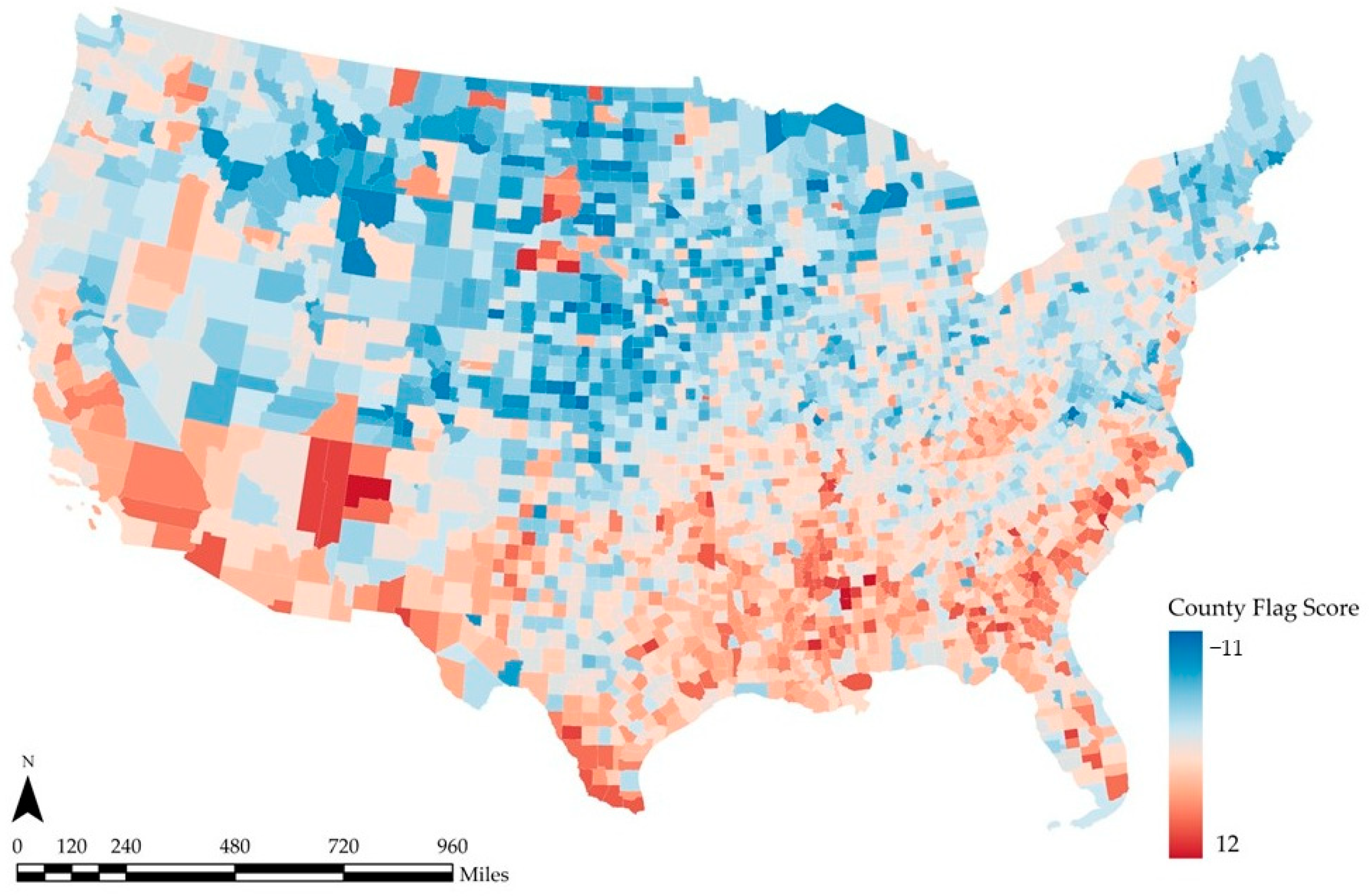
The “Flagscore” was used to construct the Livelihood Vulnerability Index by combining multiple dimensions of vulnerability into a single composite measure [29,30,54]. The Flagscore facilitates comparisons by summarizing multiple dimensions of vulnerability into a single interpretable classification measure. The Flagscore-based Livelihood Vulnerability Index was computed using a percentile-based 20–60–20 scoring system across 3109 U.S. counties: for each variable, counties in the top 20% received +1 (high-vulnerability), the bottom 20% received −1 (low-vulnerability), and the middle 60% were assigned 0 (Figure 2). The 20% threshold was strategically selected to isolate the upper and lower quintiles of the distribution. This quintile-based classification aligns with established methodological precedents in spatial epidemiology and social vulnerability research [29,30]. Specifically, foundational frameworks like the CDC’s Social Vulnerability Index (SVI) frequently utilize upper quintile (top 20%) cutoffs to identify populations disproportionately burdened by compounded risks. Spatial vulnerability rarely operates linearly; rather, structural disadvantages and adaptive failures compound exponentially at the extremes of the socio-economic spectrum. By focusing on the top and bottom 20%, the classification captures these acute vulnerability tails while avoiding the dilution of effects that occurs when overclassifying mid-range observations. Furthermore, a preliminary sensitivity check using a 25% (quartile) threshold yielded consistent directional associations, confirming the empirical robustness of this classification. Values were summed to derive the cumulative Flagscore, with higher scores indicating greater livelihood vulnerability. The resulting Flagscore was then used to classify counties by vulnerability status for the group comparison analysis. For the adjusted group comparison, counties classified as low-vulnerability and high-vulnerability were retained, while middle-range counties were excluded from the ANCOVA in order to focus on the contrast between the two extreme groups. This study incorporated 16 indicators covering demographic, economic, and health-related conditions, including the following: the percentage of non-White residents; housing vacancy rate; median building age; per capita income; education level (percent without a high school diploma); percent of workforce in manufacturing/construction (secondary industries); median housing value; household crowding rate; public transit usage; long commute share; vehicle ownership rate; population density; COVID-19 confirmed case rate; COVID-19 death rate; and accompanying socio-economic statistics like unemployment rate and poverty rate.
A Livelihood Vulnerability Index consisting of 16 variables was calculated for each county to assess susceptibility. An elevated score on this indicator signifies an increased level of susceptibility. Each county was classified as either a low-risk area (0) or a high-risk area (1) using the Flagscore. This classification, based on the Flagscore, resulted in 863 counties (48.6%) categorized as low-risk areas and 914 counties (51.4%) categorized as high-risk areas out of the total 1777 counties (a total of 42,742 census tracts) analyzed. The final analytic sample differed across models because each analysis required a different set of variables. The ANCOVA was estimated at the county level using low-vulnerability and high-vulnerability counties with valid values for the dependent variable and the covariate, whereas the multilevel models were estimated on a more restrictive complete-case sample requiring all tract level and county level predictors.

3.3. Analysis of Covariance (ANCOVA)

Analysis of Covariance (ANCOVA) is a general linear modeling approach used to assess whether mean differences between groups remain after adjustment for variance associated with a continuous covariate. By combining the comparison of group means with regression-based covariate control, ANCOVA permits estimation of the group effect while accounting for pre-existing differences on the covariate. In the present study, ANCOVA was employed to examine whether mean expenditure change differed between low-vulnerability and high-vulnerability counties after controlling for variation in county demographic composition. The dependent variable was the percentage change in total consumer expenditure between 2020 and 2022, calculated as ( E x p e n d i t u r e 2022 E x p e n d i t u r e 2020 ) / E x p e n d i t u r e 2020 × 100 . To mitigate potential distributional issues and non-normality inherent in economic shock data, the dependent variable was Winsorized at the 1st and 99th percentiles. This adjustment ensures that extreme, highly localized consumption spikes or drops do not distort the aggregate spatial vulnerability mechanisms being modeled. Middle-range counties were excluded so that the comparison focused on the contrast between the two extreme vulnerability groups [55].
In the present analysis, ANCOVA was used as a supplementary rather than primary modeling strategy. Its purpose was to examine whether the difference in expenditure change between low- and high-vulnerability counties remained after adjusting for racial composition, operationalized as the proportion of the non-White population. We retained this variable as the sole covariate because it captures an important structural dimension of disadvantage in the U.S. context, whereas additional covariates would overlap conceptually and empirically with factors already incorporated into the LVI framework. The ANCOVA results are therefore interpreted as supplementary covariate-adjusted comparisons, while the primary explanatory framework of the study remains the multilevel model [56].

3.4. Multilevel Analysis

A multilevel analysis was conducted to examine factors associated with expenditure change at both the county and census tract level simultaneously. This study employed a multilevel mixed-effects model with random intercepts to simultaneously consider both census tract level characteristics (Level 1) and county level factors (Level 2). The multilevel model accounts for the possibility that the mean value of changes in consumption varies between counties, introducing random intercepts to capture county level variations. Specifically, the Level 2 random intercept model includes both fixed effects for variables at the census tract and county levels and random effects that allow intercepts to vary across counties.
The full model includes seven census tract level factors and seven county level factors. Flagscore was used only for county classification in the group comparison analysis and was not included in the multilevel regression model. This approach allowed for an accurate assessment of how factors at both the census tract and county levels contribute to changes in consumption, accounting for regional differences and the hierarchical structure of the data. Within this hierarchical model, census-tract demographic, economic, and housing conditions were estimated together with county level mobility, density, crowding, and pandemic-burden variables [57]. The model is specified as follows:
L e v e l   1 : Y i j = β 0 j + β 1 X 1 i j + + β k X k i j + ε i j
L e v e l   2 : β 0 j = γ 0 + γ 1 M 1 j + + γ r M r j + μ 0 j
Y i j = γ 00 + β 1 X 1 i j + + β k X k i j + γ 1 M 1 j + + γ r M r j + μ o j + ε i j
where Yij represents the percentage change (%) in total consumer expenditure for the census tract i in county j between 2020 and 2022 (dependent variable), calculated as ( E x p e n d i t u r e 2022 E x p e n d i t u r e 2020 ) / E x p e n d i t u r e 2020 × 100 . γ0 is the overall intercept, μ0j is the random intercept for county j, X1ij through Xkij are k census tract level predictor variables, and M1j through Mmj are the r county level predictor variables.
Before estimating the full model, a null model was fitted to assess whether expenditure changes varied across counties prior to the inclusion of tract level and county level predictors. A random-intercept model was then estimated because census tracts are nested within counties, allowing tracts within the same county to share contextual variance while the intercept varies across counties. In this study, Level 1 variables represent census-tract demographic, economic, and housing conditions, whereas Level 2 variables represent county level mobility, density, crowding, and pandemic burden. This specification allows tract level and county level associations with expenditure change to be estimated simultaneously within a single hierarchical framework.

4. Results

4.1. ANCOVA Results

The ANCOVA results presented in Table 2 provide a supplementary comparison between low-vulnerability and high-vulnerability counties. After accounting for the proportion of the non-White population, the high-vulnerability group showed a lower mean expenditure change than the low-vulnerability group. The group effect was statistically significant ( F = 5.61 , p = 0.018 ), although the size of the difference remained modest ( η 2 = 0.010 ; adjusted R 2 = 0.012 ). The adjusted means were 9.620 for the low-vulnerability group and 9.600 for the high-vulnerability group, indicating a difference of 0.02. This result is therefore interpreted as supplementary evidence rather than as the main explanatory finding of the study.

4.2. Multilevel Analysis (Null Model)

The null model was estimated to assess the extent to which expenditure change varied between counties before the inclusion of tract level and county level predictors. The estimated county level variance was 0.0003, and the residual variance was 0.0041, yielding an intraclass correlation coefficient (ICC) of 0.067. This indicates that approximately 6.7% of the variance in expenditure change lay between counties, while the remaining variance was observed at the census-tract level. Although most of the variation was located within counties, the between-county share was not negligible, supporting the use of a multilevel specification for the present hierarchical dataset (Table 3).
The null model also yielded a log-likelihood of 28,655.75, an AIC of −57,305.51, and a BIC of −57,281.52. These statistics facilitate comparison between the null and full models under the revised specification.

4.3. Multilevel Analysis Results

Prior to estimating the full model, standard diagnostic checks were performed to ensure model validity. Variance inflation factors (VIF) for all predictors were examined, with the maximum VIF well below the critical threshold of 3.0 (Max VIF = 2.63), indicating no severe multicollinearity. Furthermore, an examination of the Level 1 and Level 2 residuals confirmed that assumptions of normality and homoscedasticity were adequately met. The subsequent multilevel analysis showed that several census-tract level and county level factors were significantly associated with expenditure change (Table 4). At the census tract level, the proportion of non-White population, vacancy rate, built year, per capita income, and housing value were statistically significant, whereas educational attainment and employment in secondary industries were not significant. At the county level, confirmed COVID-19 cases, COVID-19 deaths, overcrowded households, public transportation use, and the proportion of households without a vehicle had significant coefficients, whereas commute time and population density did not reach statistical significance.
At the county level, the number of confirmed COVID-19 cases and death cases were positively associated with expenditure change. Overcrowded households and the proportion of households without a vehicle were negatively associated with expenditure change, whereas public transportation use showed a positive association. Commute time and population density were not statistically significant. These findings indicate that county level contextual conditions were linked to expenditure change in different ways rather than producing a uniform pattern across all counties.

4.4. Research Limitations

This study provides a multilevel analysis of the relationship between county and census-tract level spending changes and Livelihood Vulnerability indicators across the United States. Supporting our expenditure measures, the Bureau of Labor Statistics’ Consumer Expenditure Survey (CEX) relies on self-reported diaries and interviews and may not fairly represent actual household activities. Particularly underrepresented are demographics like contingent workers and small-business owners, who would have experienced the most notable consumption shocks, hence causing a downward bias in the expected spending declines. Moreover, our Livelihood Vulnerability Index (LVI) aggregates 16 indicators with equal weighting, which may obscure the differing importance of individual components across regions. The county classification also relied on a 20% threshold rule, and alternative cutpoint specifications were not tested in the present analysis. Therefore, our statistical models may not fully reflect geographical or seasonally distinct vulnerabilities that could greatly influence expenditure patterns. Future research should examine the robustness of the classification under different threshold choices.
Second, the study’s cross-sectional comparison of 2020 and 2022 spending data limits our ability to trace the dynamic evolution of consumption behaviors throughout and after the pandemic. We do not address the speed of recovery, the emergence of long-term adaptation strategies, or the effects of seasonality on household expenditures. In the end, the conclusions might not be relevant to smaller governments or various national environments since our study is limited to vast U.S. data. Higher-frequency time-series data, explicitly modeling geographical dependency, and cross-country or subnational comparative analysis will all help future research to increase the generalizability and resilience of conclusions.

5. Discussion

This study links pre-existing vulnerability conditions to changes in consumer expenditure at both the census-tract and county levels. By combining county classification with multilevel analysis, it shows that expenditure change depended on both neighborhood-level socio-economic conditions and broader county-level contextual factors. Compared with approaches relying only on aggregate retail recovery, this design provides a more localized view of uneven economic strain during the COVID-19 period.
At the census-tract level, demographic composition (non-White population share) [21,58] and physical infrastructure constraints (vacancy rates and declining building stocks) emerged as significant predictors of expenditure loss, while individual human capital factors like education were not significant. This indicates that local economic resilience was constrained more heavily by ingrained spatial and housing inequalities than by individual socio-economic status. By explicitly isolating this pre-health economic vulnerability, the study clarifies how livelihood-related structural risks shape communities’ ability to maintain essential expenditures under sustained disruption. Even so, mapping where households lose the capacity to maintain basic spending is a practical first step for targeting public-health resources, since the same communities are often those with the least room to invest in preventive care.
Second, the multilevel approach of this study clarifies the different effects of COVID-19-related mobility features and health outcomes at the county level. Previous studies stressing the compounding effects of health crises on underprivileged populations match the clear linkages among COVID-19 cases, death rates, and economic disruptions [6]. At the same time, the county level coefficients did not move in a single direction. Public transportation use carried a positive coefficient, whereas crowding and the proportion of households without a vehicle were linked to lower expenditure growth. The positive association of public transit suggests that maintaining access to functional transit networks served as a vital lifeline, enabling essential workers to sustain their livelihoods and economic activities during the crisis. In contrast, the negative impact of vehicle deprivation highlights the severe economic isolation faced by households lacking private mobility when lockdowns disrupted local services. These divergent outcomes do not point to a uniform decline but instead reflect how mobility-related structural conditions dictate a community’s capacity for adaptive adjustment.
The tract-level and county-level results jointly suggest that expenditure change reflected multiple dimensions of vulnerability rather than a single uniformly operating factor. Demographic and housing-related conditions mattered at the tract level, while pandemic burden and mobility-related conditions remained relevant at the county level, although not always in the same direction.
While our cross-sectional design precludes the empirical testing of causal pathways, the observed negative associations between built-environment constraints—such as high vacancy rates, declining housing stock, and a lack of mobility options—and expenditure loss are theoretically consistent with the concept of spatial poverty traps [59]. The results strongly suggest a scenario where households in structurally disadvantaged areas facing a health crisis, the high fixed costs associated with navigating inadequate infrastructure crowds out essential consumer spending. Consequently, resilience planning requires specific spatial interventions rather than generic stimulus. Urban planners should integrate consumption capacity into land-use decisions. For instance, implementing mixed-use zoning and transit-oriented development (TOD) in high-LVI tracts mitigates the negative impact of vehicle deprivation, directly freeing up household budgets to absorb unexpected economic disruptions. Coordinating these spatial reconfigurations with localized service delivery, such as deploying mobile health units in transportation deserts, addresses the physical and economic constraints simultaneously.
Future research directions could include longitudinal studies tracking post-pandemic recovery trajectories at local levels and incorporating real-time mobility and socio-economic data to enhance predictive modeling. Comparative studies across several geographical settings can also provide insights into resilience strategies that are globally relevant as opposed to those unique to each location. A natural next step would be to connect the consumption–vulnerability patterns found here with actual health outcomes, such as avoidable hospitalizations or mental health service use, to test whether the economic shocks documented at the county and tract levels do, in fact, widen health disparities. This work lays a strong foundation for such extensions by clearly demonstrating the need for localized vulnerability assessments to be included in comprehensive resilience planning systems [60,61,62,63].

6. Conclusions

This study examined how livelihood vulnerability and local contextual conditions were associated with changes in consumer expenditure across U.S. census tracts and counties during the COVID-19 pandemic. A county level Livelihood Vulnerability Index (LVI) was constructed to classify counties for group comparison, and a multilevel model was then estimated to identify the census tract level and county level factors associated with expenditure change. This framework separates local neighborhood conditions from broader county level pandemic and mobility contexts in explaining uneven expenditure outcomes.
At the census tract level, expenditure change was related to demographic composition, housing conditions, and local income levels. Educational attainment and secondary-industry employment, by contrast, were not significant. At the county level, confirmed cases, death cases, public transportation use, crowding, and the proportion of households without a vehicle were statistically significant, confirming that pandemic burden and mobility-related conditions shaped local spending trajectories.
At the county level, pandemic burden and mobility-related conditions played a measurable role in expenditure outcomes, but their effects were not uniformly negative. In particular, confirmed cases and death cases bore a strong relationship to expenditure shifts over the 2020–2022 period, suggesting that county level pandemic severity remained an important contextual factor in local spending trajectories. At the same time, crowding and lack of vehicle access were linked to lower expenditure growth, whereas public transit use carried a positive coefficient. These findings suggest that resilience planning should account for both neighborhood disadvantage and broader county level contextual conditions.
The main contribution of this study lies in showing how pre-existing county level vulnerability and tract level local conditions were linked to uneven expenditure change during the COVID-19 period within a single multilevel framework. Instead of relying only on aggregate recovery indicators, the analysis uses expenditure change as a closer approximation of household-level economic strain and shows that this strain was associated with both neighborhood disadvantage and broader county level pandemic and mobility conditions. The findings therefore add specificity to resilience research by identifying how vulnerability operated across nested spatial scales instead of treating local economic disruption as a uniform outcome.

Author Contributions

Conceptualization, Seongbeom Park; methodology, Seongbeom Park; writing—original draft preparation, Seongbeom Park; data curation, Jong Ho Won; formal analysis, Jong Ho Won; visualization, Jong Ho Won; writing—review and editing, Jaekyung Lee; project administration, Jaekyung Lee; supervision, Jaekyung Lee. All authors have read and agreed to the published version of the manuscript.

Funding

This work was supported by the Ministry of Education of the Republic of Korea and the National Research Foundation of Korea (NRF-2024S1A5A2A03038101).

Data Availability Statement

The data that support the findings of this study were obtained under license through EASI and are not publicly available due to licensing restrictions. Data may be available from the authors upon reasonable request and with permission from EASI, subject to the license terms.

Conflicts of Interest

The authors declare no competing financial interests.

References

  1. Sharifi, A.; Khavarian-Garmsir, A.R. The COVID-19 pandemic: Impacts on cities and major lessons for urban planning, design, and management. Sci. Total Environ. 2020, 749, 142391. [Google Scholar] [CrossRef] [Scilit]
  2. Mora, L.; Deakin, M.; Reid, A. Strategic principles for smart city development: A multiple case study analysis of European best practices. Technol. Forecast. Soc. Change 2019, 142, 70–97. [Google Scholar] [CrossRef] [Scilit]
  3. Holling, C.S. Resilience and Stability of Ecological Systems. Annu. Rev. Ecol. Syst. 1973, 4, 1–23. [Google Scholar] [CrossRef] [Scilit]
  4. Folke, C.; Carpenter, S.R.; Walker, B.; Scheffer, M.; Chapin, T.; Rockström, J. Resilience thinking: Integrating resilience, adaptability and transformability. Ecol. Soc. 2010, 15, 20. [Google Scholar] [CrossRef] [Scilit]
  5. Chetty, R.; Friedman, J.N.; Stepner, M. The Economic Impacts of COVID-19: Evidence from a New Public Database Built Using Private Sector Data. Q. J. Econ. 2022, 139, 829–889. [Google Scholar] [CrossRef] [Scilit] [PubMed]
  6. Patel, J.A.; Nielsen, F.B.H.; Badiani, A.A.; Assi, S.; Unadkat, V.A.; Patel, B.; Ravindrane, R.; Wardle, H. Poverty, inequality and COVID-19: The forgotten vulnerable. Public Health 2020, 183, 110–111. [Google Scholar] [CrossRef] [Scilit]
  7. Williams, D.R.; Lawrence, J.A.; Davis, B.A. Racism and Health: Evidence and Needed Research. Annu. Rev. Public Health 2019, 40, 105–125. [Google Scholar] [CrossRef] [Scilit]
  8. Fairlie, R. The impact of COVID-19 on small business owners: Evidence from the first three months after widespread social-distancing restrictions. J. Econ. Manag. Strategy 2020, 29, 727–740. [Google Scholar] [CrossRef] [Scilit]
  9. Massey, D.S.; Denton, N.A. American apartheid: Segregation and the making of the underclass. In Social Stratification, Class, Race, and Gender in Sociological Perspective, 2nd ed.; Routledge: Abingdon, UK, 2019; pp. 660–670. [Google Scholar]
  10. Holling, C.S.; Gundersen, L.H. Resilience and Adaptive Cycles; Island Press: Washington, DC, USA, 2002. [Google Scholar]
  11. Van Meerbeek, K.; Jucker, T.; Svenning, J.C. Unifying the concepts of stability and resilience in ecology. J. Ecol. 2021, 109, 3114–3132. [Google Scholar] [CrossRef] [Scilit]
  12. Pendall, R.; Foster, K.A.; Cowell, M. Resilience and regions: Building understanding of the metaphor. Camb. J. Reg. Econ. Soc. 2009, 3, 71–84. [Google Scholar] [CrossRef] [Scilit]
  13. Cui, P.; Dong, Z.; Yao, X.; Cao, Y.; Sun, Y.; Feng, L. What Makes Urban Communities More Resilient to COVID-19? A Systematic Review of Current Evidence. Int. J. Environ. Res. Public Health 2022, 19, 10532. [Google Scholar] [CrossRef] [Scilit] [PubMed]
  14. Campanella, T.J. Urban resilience and the recovery of New Orleans. J. Am. Plan. Assoc. 2006, 72, 141–146. [Google Scholar] [CrossRef] [Scilit]
  15. Meerow, S.; Newell, J.P.; Stults, M. Defining urban resilience: A review. Landsc. Urban Plan. 2016, 147, 38–49. [Google Scholar] [CrossRef] [Scilit]
  16. U.S. Bureau of Labor Statistics. Leisure and Hospitality Employment Down 2.1 Percent from February 2020 Level; U.S. Bureau of Labor Statistics: Washington, DC, USA, 2023. Available online: https://www.bls.gov/opub/ted/2023/leisure-and-hospitality-employment-down-2-1-percent-from-february-2020-level.htm (accessed on 28 April 2025).
  17. Economic Policy Institute. Only One in Five Workers Are Working from Home Due to COVID: Black and Hispanic Workers Are Less Likely to Be Able to Telework; Economic Policy Institute: Washington, DC, USA, 2021; Available online: https://www.epi.org/blog/only-one-in-five-workers-are-working-from-home-due-to-covid-black-and-hispanic-workers-are-less-likely-to-be-able-to-telework/ (accessed on 28 April 2025).
  18. Turner, B.L.; Kasperson, R.E.; Matson, P.A.; McCarthy, J.J.; Corell, R.W.; Christensen, L.; Eckley, N.; Kasperson, J.X.; Luers, A.; Martello, M.L.; et al. A framework for vulnerability analysis in sustainability science. Proc. Natl. Acad. Sci. USA 2003, 100, 8074–8079. [Google Scholar] [CrossRef] [Scilit]
  19. Varshney, K.; Glodjo, T.; Adalbert, J. Overcrowded housing increases risk for COVID-19 mortality: An ecological study. BMC Res. Notes 2022, 15, 126. [Google Scholar] [CrossRef] [Scilit]
  20. Kaiser Family Foundation. COVID-19 Cases and Deaths by Race/Ethnicity: Current Data and Changes over Time; Kaiser Family Foundation: San Francisco, CA, USA, 2022; Available online: https://www.kff.org/racial-equity-and-health-policy/issue-brief/covid-19-cases-and-deaths-by-race-ethnicity-current-data-and-changes-over-time/ (accessed on 28 April 2025).
  21. Massey, D.S.; Denton, N.A. Hypersegregation in US metropolitan areas: Black and Hispanic segregation along five dimensions. Demography 1989, 26, 373–391. [Google Scholar] [CrossRef] [Scilit]
  22. Cheng, B.; Kim, A. Delayed or Forgone Medical Care due to COVID-19 among Adults and Children with Atopic Dermatitis. J. Allergy Clin. Immunol. 2023, 151, AB154. [Google Scholar] [CrossRef] [Scilit]
  23. Mein, S.A.; Marinacci, L.X.; Zheng, Z.; Ahmad, I.; Wadhera, R.K. Changes in health care and prescription medication affordability in the US During the COVID-19 pandemic. In JAMA Health Forum; American Medical Association: Chicago, IL, USA, 2024. [Google Scholar]
  24. Li, M.; Harmon, M.; Wasson, M.; Cardosi, L.; Henson, L.; Hill, H.; Jobe, B.I.; Hewitt, S.E.; Hohmeier, K.C. Abandonment of prescriptions in medically underserved areas: Primary medication non-adherence in community pharmacies in the delta region of the United States. Explor. Res. Clin. Soc. Pharm. 2024, 15, 100484. [Google Scholar] [CrossRef] [Scilit]
  25. Sen, A. Development as freedom. Dev. Pract.-Oxf. 2000, 10, 258. [Google Scholar]
  26. Sen, A. On Ethics and Economics; Oxford University Press: Oxford, UK, 1999. [Google Scholar]
  27. Robeyns, I. The capability approach: A theoretical survey. J. Hum. Dev. 2005, 6, 93–117. [Google Scholar] [CrossRef] [Scilit]
  28. Gershenson, C.; Desmond, M. Eviction and the Rental Housing Crisis in Rural America☆. Rural Sociol. 2024, 89, 86–105. [Google Scholar] [CrossRef] [Scilit]
  29. Cutter, S.L.; Boruff, B.J.; Shirley, W.L. Social vulnerability to environmental hazards. Soc. Sci. Q. 2003, 84, 242–261. [Google Scholar] [CrossRef] [Scilit]
  30. Flanagan, B.E.; Gregory, E.W.; Hallisey, E.J.; Heitgerd, J.L.; Lewis, B. A social vulnerability index for disaster management. J. Homel. Secur. Emerg. Manag. 2011, 8, 3. [Google Scholar] [CrossRef] [Scilit]
  31. Fatemi, F.; Ardalan, A.; Aguirre, B.; Mansouri, N.; Mohammadfam, I. Social vulnerability indicators in disasters: Findings from a systematic review. Int. J. Disaster Risk Reduct. 2017, 22, 219–227. [Google Scholar] [CrossRef] [Scilit]
  32. Park, S.; Lee, J.; Park, Y. Analysis of residential satisfaction changes by the land bank program using text mining. Sustainability 2022, 14, 11707. [Google Scholar] [CrossRef] [Scilit]
  33. Chuang, W.-C.; Gober, P. Predicting hospitalization for heat-related illness at the census-tract level: Accuracy of a generic heat vulnerability index in Phoenix, Arizona (USA). Environ. Health Perspect. 2015, 123, 606–612. [Google Scholar] [CrossRef] [Scilit] [PubMed]
  34. Mortensen, D.T.; Nagypal, E. More on unemployment and vacancy fluctuations. Rev. Econ. Dyn. 2007, 10, 327–347. [Google Scholar] [CrossRef] [Scilit]
  35. Oulahen, G.; Mortsch, L.; Tang, K.; Harford, D. Unequal vulnerability to flood hazards: “Ground truthing” a social vulnerability index of five municipalities in Metro Vancouver, Canada. Ann. Assoc. Am. Geogr. 2015, 105, 473–495. [Google Scholar] [CrossRef] [Scilit]
  36. Holcombe, R.G.; Lacombe, D.J. The effect of state income taxation on per capita income growth. Public Financ. Rev. 2004, 32, 292–312. [Google Scholar] [CrossRef] [Scilit]
  37. Hasan, M.S. The long-run relationship between population and per capita income growth in China. J. Policy Model. 2010, 32, 355–372. [Google Scholar] [CrossRef] [Scilit]
  38. Amos, J. Dropouts, Diplomas, and Dollars: US High Schools and the Nation’s Economy; Alliance for Excellent Education: Washington, DC, USA, 2008. [Google Scholar]
  39. Tate, E. Social vulnerability indices: A comparative assessment using uncertainty and sensitivity analysis. Nat. Hazards 2012, 63, 325–347. [Google Scholar] [CrossRef] [Scilit]
  40. Chen, W.; Cutter, S.L.; Emrich, C.T.; Shi, P. Measuring social vulnerability to natural hazards in the Yangtze River Delta region, China. Int. J. Disaster Risk Sci. 2013, 4, 169–181. [Google Scholar] [CrossRef] [Scilit]
  41. Kain, J.F.; Quigley, J.M. Measuring the value of housing quality. J. Am. Stat. Assoc. 1970, 65, 532–548. [Google Scholar] [CrossRef]
  42. Wood, N.J.; Burton, C.G.; Cutter, S.L. Community variations in social vulnerability to Cascadia-related tsunamis in the U.S. Pacific Northwest. Nat. Hazards 2009, 52, 369–389. [Google Scholar] [CrossRef] [Scilit]
  43. Díaz McConnell, E. Rented, crowded, and unaffordable? Social vulnerabilities and the accumulation of precarious housing conditions in Los Angeles. Hous. Policy Debate 2017, 27, 60–79. [Google Scholar] [CrossRef] [Scilit]
  44. Ríos, V.; Denova-Gutiérrez, E.; Barquera, S. Association between living in municipalities with high crowding conditions and poverty and mortality from COVID-19 in Mexico. PLoS ONE 2022, 17, e0264137. [Google Scholar] [CrossRef] [Scilit]
  45. Gebremeskel, E.; Woldeamanuel, M.; Woldetensae, B. Transport vulnerability: Measuring travel time and expenditure budget in Addis Ababa. Res. Transp. Econ. 2023, 100, 101247. [Google Scholar] [CrossRef] [Scilit]
  46. Verbich, D.; El-Geneidy, A. Public transit fare structure and social vulnerability in Montreal, Canada. Transp. Res. Part A Policy Pract. 2017, 96, 43–53. [Google Scholar] [CrossRef] [Scilit]
  47. Besser, L.M.; Marcus, M.; Frumkin, H. Commute time and social capital in the US. Am. J. Prev. Med. 2008, 34, 207–211. [Google Scholar] [CrossRef] [Scilit]
  48. Sullivan, J.L.; Novak, D.C. A method for evaluating accessibility in transportation problems considering social vulnerability. Eur. J. Oper. Res. 2024, 317, 646–659. [Google Scholar] [CrossRef] [Scilit]
  49. Rufat, S.; Tate, E.; Emrich, C.T.; Antolini, F. How Valid Are Social Vulnerability Models? Ann. Am. Assoc. Geogr. 2019, 109, 1131–1153. [Google Scholar] [CrossRef] [Scilit] [PubMed]
  50. Batabyal, S.; McCollum, M. Should population density be used to rank social vulnerability in disaster preparedness planning? Econ. Model. 2023, 125, 106165. [Google Scholar] [CrossRef] [Scilit]
  51. de Oliveira Mendes, J.M. Social vulnerability indexes as planning tools: Beyond the preparedness paradigm. J. Risk Res. 2009, 12, 43–58. [Google Scholar] [CrossRef] [Scilit]
  52. Nayak, A.; Islam, S.J.; Mehta, A.; Ko, Y.A.; Patel, S.A.; Goyal, A.; Sullivan, S.; Lewis, T.T.; Vaccarino, V.; Morris, A.A.; et al. Impact of social vulnerability on COVID-19 incidence and outcomes in the United States. MedRxiv 2020. [Google Scholar] [CrossRef] [Scilit]
  53. Khazanchi, R.; Beiter, E.R.; Gondi, S.; Beckman, A.L.; Bilinski, A.; Ganguli, I. County-level association of social vulnerability with COVID-19 cases and deaths in the USA. J. Gen. Intern. Med. 2020, 35, 2784–2787. [Google Scholar] [CrossRef] [Scilit]
  54. Berke, P.; Newman, G.; Lee, J.; Combs, T.; Kolosna, C.; Salvesen, D. Evaluation of Networks of Plans and Vulnerability to Hazards and Climate Change: A Resilience Scorecard. J. Am. Plan. Assoc. 2015, 81, 287–302. [Google Scholar] [CrossRef] [Scilit]
  55. Van Breukelen, G.J. ANCOVA versus change from baseline had more power in randomized studies and more bias in nonrandomized studies. J. Clin. Epidemiol. 2006, 59, 920–925. [Google Scholar] [CrossRef] [Scilit]
  56. Miller, G.A.; Chapman, J.P. Misunderstanding analysis of covariance. J. Abnorm. Psychol. 2001, 110, 40–48. [Google Scholar] [CrossRef]
  57. Roux, A.D. A glossary for multilevel analysis. J. Epidemiol. Community Health 2002, 56, 588–594. [Google Scholar] [CrossRef] [Scilit]
  58. Lichter, D.T.; Parisi, D.; Taquino, M.C. Toward a new macro-segregation? Decomposing segregation within and between metropolitan cities and suburbs. Am. Sociol. Rev. 2015, 80, 843–873. [Google Scholar] [CrossRef] [Scilit]
  59. Bird, K.; Higgins, K.; Harris, D. Spatial Poverty Traps: An Overview; Overseas Development Institute: London, UK, 2010. [Google Scholar]
  60. Statista. Poverty Rate in the United States from 1990 to 2023. 2024. Available online: https://www.statista.com/statistics/200463/us-poverty-rate-since-1990/ (accessed on 28 April 2025).
  61. Clark, D.; Marianna, S. Biden Lays Out $1.9 Trillion COVID-19 Relief Package. NBC News, 14 January 2021. Available online: https://www.nbcnews.com/politics/politics-news/biden-lays-out-1-9-trillion-covid-19-relief-package-n1254334 (accessed on 28 April 2025).
  62. Burns, K.; DiTommaso, A. Poverty Measure That Includes Noncash Government Assistance Increased to 12.9% in 2023, Up from 12.4% in 2022; U.S. Census Bureau: Suitland, MD, USA, 2024. Available online: https://www.census.gov/library/stories/2024/09/supplemental-poverty-measure.html (accessed on 28 April 2025).
  63. First Focus on Children. Child Poverty in 2023: Issue Brief; First Focus on Children: Washington, DC, USA, 2024. [Google Scholar]
Figure 1. National trends in the U.S. poverty rate and monthly COVID-19 deaths, 2020–2022. This figure is included to illustrate the broader public health and material-hardship context within which local expenditure change is examined (data source: CDC COVID Data Tracker; U.S. Census Bureau).
Ijgi 15 00183 g001
Figure 2. County Flagscore Distribution across 3109 U.S. counties—Flagscore is calculated as the sum of percentile-based 20–60–20 indicator scores: counties in the top 20% of each indicator receive +1, counties in the bottom 20% receive −1, and counties in the middle 60% receive 0; higher values indicate greater livelihood vulnerability (Map projection: NAD 1983 Contiguous USA Albers).
Ijgi 15 00183 g002
Table 2. ANCOVA summary and adjusted means for percentage change (%) in total consumer expenditure by vulnerability group.
TermObs.CovariateFp-Value η 2 Adjusted   R 2 Adjusted Means
LowHigh
Risk_group1463Proportion of the non-White population5.610.0180.0100.0129.6209.600
The ANCOVA was estimated on county level observations with valid values for the dependent variable and covariate in the low-vulnerability and high-vulnerability groups.
Table 3. Null model results and model-fit statistics for the revised multilevel specification.
Random Effects
GroupsNameVarianceStd. Dev
CountyID(Intercept)0.00030.0173
Residual 0.00410.0642
Obs:27,016Groups:1495
Model Fit
ICCLog-LikelihoodAICBIC
0.06728,655.75−57,305.51−57,281.52
The null model was estimated on the complete-case multilevel analytic sample (27,016 census tracts nested within 1495 counties).
Table 4. Multilevel analysis results.
Fixed Effects
No. Observations:27,016Dependent
Variable:
Percentage change (%) in total
consumer expenditure, 2020–2022
No. Groups:1495 Method:REML
Min. group size:1 Scale:0.0353
Max. group size:662 Log-Likelihood:6145.7698
CoefStd. Errzp > |z|[0.025 0.975]
Level 1. Census Tract
Intercept9.5860.0032831.03509.5799.593
Non-White−0.0070.002−3.6320−0.01−0.003
Vacancy−0.0060.002−3.5260−0.009−0.002
Average building year−0.0270.002−13.50−0.03−0.024
Per Capita Income0.0130.0026.14200.0090.018
Education (No high school diploma)0.0010.0020.50.6171−0.0030.004
Employment (Secondary industries)0.0010.0020.50.6171−0.0020.004
Housing Value0.0070.0023.50.0050.0030.012
Level 2. County
Confirmed Cases0.0090.0033.420.0010.0040.014
Death Cases0.0080.0033.0170.0030.0030.013
Crowding−0.0040.002−20.04−0.008−0.001
Public Transportation0.0080.0032.6670.0080.0020.014
Commute Time
(>30min)
00.0030.0530.958−0.0060.006
Households without a vehicle−0.0070.003−2.5970.009−0.012−0.002
Population Density−0.0020.005−0.4070.284−0.0120.008
The full multilevel model was estimated on the same complete-case analytic sample as the null model (27,016 census tracts nested within 1495 counties).
Disclaimer/Publisher’s Note: The statements, opinions and data contained in all publications are solely those of the individual author(s) and contributor(s) and not of MDPI and/or the editor(s). MDPI and/or the editor(s) disclaim responsibility for any injury to people or property resulting from any ideas, methods, instructions or products referred to in the content.