A Large Language Model for Traffic Flow Prediction Based on Stationary Wavelet Transform and Graph Convolutional Networks

Abstract

With the rapid development of Intelligent Transportation Systems (ITSs), traffic prediction, a crucial component of ITSs, has garnered growing scholarly attention. The appli-cation of deep learning into traffic prediction has emerged as a prominent research direction, especially amid the rapid advancement of pretrained large language models (LLMs), which offer substantial benefits in time-series analysis through cross-modal knowledge transfer. In response to this advancement, this study introduces an innovative model for traffic flow prediction, designated as WGLLM. To capture spatiotemporal characteristics inherent in traffic flow data, this model incorporates a sequence embedding layer constructed on the stationary wavelet transform (SWT) and long short-term memory (LSTM), in conjunction with a spatial embedding layer founded on graph convolutional networks (GCNs). Additionally, a fully connected layer is utilized to integrate embeddings into the LLMs for comprehensive global dependency analysis. To verify the effectiveness of the proposed approach, experiments were carried out on two real traffic flow datasets. The experimental results demonstrate that WGLLM achieves superior predictive performance compared to multiple mainstream baseline models, accompanied by a significant enhancement in prediction accuracy.

1. Introduction

As a key component in coordinating urban transportation, Intelligent Transportation Systems (ITSs) are rapidly developing, providing effective solutions for the construction and development of digital transportation. The core goal of ITSs is to deliver participants with a high-performance transportation system, including optimal traffic signal control, traffic flow control, and autonomous vehicle control [1]. Traffic forecasting is a core component of ITSs [2]. By analyzing and modeling historical traffic data, it predicts future traffic conditions, which is crucial for traffic condition analysis and traffic safety. Additionally, traffic prediction is important to travelers, assisting them in planning their routes in advance, selecting the optimal travel time, and improving travel efficiency. Consequently, numerous researchers have developed a variety of high-precision prediction techniques in this domain. Specifically, extensive efforts have been devoted to dynamic path optimization and transportation network efficiency enhancement, where time-optimized routing schemes and an adaptive congestion index-based improved A * algorithm have been developed to substantially boost network throughput and refine vehicle mobility performance [3,4]. For multi-lane and expressway ramp traffic flow modeling, the CNAT * model and continuous cellular automata approach have been established to uncover the patterns of traffic flow fluctuation, mechanisms of congestion propagation, and the effects of driving behavior on traffic operations [5,6]. In the realm of deep learning-driven traffic forecasting, prompt learning has been incorporated with graph convolutional networks to mitigate data distribution shifts and strengthen model generalization and predictive accuracy, offering a novel framework for high-precision traffic flow prediction [7].

In terms of research methods, the approaches used include series analysis, traditional machine learning models, and deep learning models. The Historical Average (HA) method [8,9] is one of the earliest statistical approaches employed in highway traffic flow prediction. Its core mechanism involves computing the average historical traffic flow data at individual traffic nodes to generate predictive outputs. Another widely utilized category of statistical methods includes the autoregressive (AR) model and its variants, among which the autoregressive integrated moving average (ARIMA) model has garnered extensive recognition for its superior time-series modeling capabilities. ARIMA’s first successful application in highway traffic flow prediction further broadened the research landscape of traffic time-series forecasting [10]. Kalman filter theory constructs filters by introducing a state-space framework for linear stochastic systems, facilitating the estimation of system states from noise-contaminated data when the measurement variances are known. Okutani and Stephanedes [11] pioneered the establishment of two short-term traffic flow forecasting approaches grounded in Kalman filter theory, which yielded favorable predictive performance. However, with the escalating deployment density of sensor devices and rapid expansion of traffic network scales, traditional statistical analysis-based time-series prediction methods have exhibited pronounced limitations. Characterized by constrained predictive accuracy, these methods are no longer adequate to fulfill the requirements of modernized transportation systems.

With the growing travel demands of residents, the nonlinear characteristics of traffic flow have become increasingly prominent, prompting the application of numerous traditional machine learning models in traffic flow prediction. The K-nearest neighbor (k-NN) model is a conventional machine learning approach employed in traffic prediction, whose core mechanism involves generating predictive outcomes by identifying the closest data points from historical records based on recent observations [12]. Support Vector Regression (SVR), a method rooted in statistical learning theory [13,14], minimizes prediction errors by determining the optimal hyperplane. However, these conventional methods exhibit three key limitations: first, they typically employ simple shallow architectures with a restricted number of learnable parameters, thereby constraining improvements in predictive performance; second, most rely on manually engineered features from traffic data, entailing substantial labor and time costs; third, many studies focus primarily on the mining of temporal features, yet lack explicit modeling of road network spatial structure, making it difficult to automatically capture the spatial correlations and dynamic propagation patterns of traffic flow.

Alongside the continuous progression of deep learning, an expanding array of deep learning-based spatiotemporal prediction methods have emerged. Recurrent neural networks (RNNs) [15] and RNN-based variant models [16,17,18] have exhibited superior performance in capturing time-related patterns from traffic flow data. For spatial feature extraction, convolutional neural networks (CNNs) efficiently capture spatial patterns via convolutional layers [19,20]. Nevertheless, these methods are unable to fully leverage the topological structure of road networks for effective extraction of spatial information associated with network nodes. Graph convolutional networks (GCNs) have mitigated this limitation. Zhao et al. [21] proposed the temporal graph convolutional network (T-GCN), an integration of vanilla graph convolutions and Gated Recurrent Units (GRUs) designed for spatiotemporal feature extraction. Similarly, to separately model spatial and temporal correlations, Yu et al. [22] developed the spatiotemporal graph convolutional network (STGCN), utilizing GCNs and 1D-CNNs. Furthermore, some scholars have incorporated attention mechanisms. For instance, Guo et al. [23] proposed the ASTGCN model to learn a dynamic spatial correlation matrix, thereby enhancing graph convolutions. Spatiotemporal synchronous graph convolutional network (STSGCN) constructs a spatiotemporal synchronous graph convolutional operator capable of simultaneously capturing information from a node’s one-hop spatial and temporal neighbors [24].

In recent years, pretrained large language models (LLMs) have exhibited remarkable efficacy across diverse natural language processing tasks [25]. OpenAI introduced the Generative Pre-trained Transformer (GPT), which is rooted in the Transformer decoder, followed by the release of newer GPT, with the latter featuring a substantially expanded parameter scale [26,27,28]. These models not only demonstrate exceptional performance across a broad spectrum of natural language processing (NLP) tasks but also demonstrate superior performance in specialized domain-specific tasks. The Frozen Pretrained Transformer (FPT), a time-series analysis framework built on pre-trained LLMs, marks the first application of such models to time-series analysis tasks [29]. However, owing to the domain discrepancy between linguistic and traffic data, where traffic flow data not only possess unique temporal characteristics but also encompass substantial non-textual information, LLMs encounter difficulties in directly extracting meaningful insights from complex traffic flow data. This constraint results in suboptimal performance in long-term prediction tasks, such as traffic flow forecasting.

To better integrate large language models (LLMs) into traffic prediction tasks, we develop a wavelet-graph enhanced LLM (WGLLM) based on a SWT and GCN. The underlying principle is to separately capture temporal characteristics and spatial attributes from traffic flow data. SWT is employed to denoise the raw data, followed by long short-term memory (LSTM) to extract long-term dependencies in data, and GCN analyzes road network structure to extract spatial features. The extracted features are then integrated and fed into LLMs to analyze global dependencies. The primary contributions of this research are summarized as follows:

(1)

This study proposes an innovative prediction model that integrates wavelet transform and GCN into LLMs to boost the model’s capacity to handle traffic prediction tasks.

(2)

Building on the wavelet transform, the model enhances the temporal features of the input sub-signals through LSTM, enabling the WGLLM to model the spatiotemporal feature interactions across different traffic data types.

(3)

We conducted experiments on the public Citi Historical Bike Dataset (CHBike) and New York City taxi dataset (NYCTaxi), and the results verify the outstanding performance of the WGLLM. Additionally, a series of ablation studies were performed to validate the incorporation of wavelet transforms, and GCNs significantly improve the model performance.

The subsequent sections of this paper are structured as follows: Section 2 presents a detailed overview of the methodologies and underlying principles associated with the WGLLM. Section 3 presents the ablation experiments and analyzes the experimental results. Section 4 and Section 5 discuss and summarize the study and outline promising avenues for subsequent research investigations.

2. Materials and Methods

2.1. Problem Definition

Since traffic flow prediction is a type of structured time series prediction, graph structures are applied to transportation networks by defining the traffic road network on a graph. The transportation network is defined herein as G = (V, E, A), where V is the vertex set, the sensor stations in the traffic road network, E is the edge set and A ∈ R^N×N is the weight matrix, representing the correlation coefficients between each pair of sensor stations in the traffic road network. This study uses ${\mathrm{x}}_{\mathrm{t}}=\{{\mathrm{x}}_1,\dots ,{\mathrm{x}}_{\mathrm{n}},\dots ,{\mathrm{x}}_{\mathrm{N}}\}\in {\mathrm{R}}^{\mathrm{N}}$ to represent the temporal features of graph G at time t, where ${\mathrm{x}}_{\mathrm{n}}$ denotes the node features data collected by sensor node n at time t, such as traffic flow and average speed.

Traffic flow prediction involves predicting the traffic flow sequence in the future time period given the traffic road network graph G and the historical traffic flow sequence over T time periods. This prediction process is based on a mapping relationship, and its core objective is to find a model $f(·)$. The prediction process is formally expressed as follows:

$$Y=f\left(X,A\right)$$

(1)

where $\mathrm{X}=\{{\mathrm{x}}_{\mathrm{t}-\mathrm{T}+1},\dots ,{\mathrm{x}}_{\mathrm{t}}\}\in {\mathrm{R}}^{\mathrm{N}\times \mathrm{T}}$ is the historical sequence of the last T time steps, $A$ is the adjacency matrix of graph G, $Y$ = {y_t+1, …, ${\mathrm{y}}_{\mathrm{t}+\mathrm{i}}$, …, ${\mathrm{y}}_{\mathrm{t}+\mathrm{T}\mathrm{’}}$} ∈ R^N×T’ is the predicted sequence for the next T′ time steps, and ${\mathrm{y}}_{\mathrm{t}+1}$∈R^N is the feature prediction value of graph G at the ${\mathrm{i}}^{\mathrm{t}\mathrm{h}}$ future time step. Based on deep learning theory, this study uses a deep learning-based approximator ${\mathrm{f}}_{\theta }(·)$ to approximate $f(·)$, where θ is a learnable parameter.

2.2. WGLLM Architecture Design

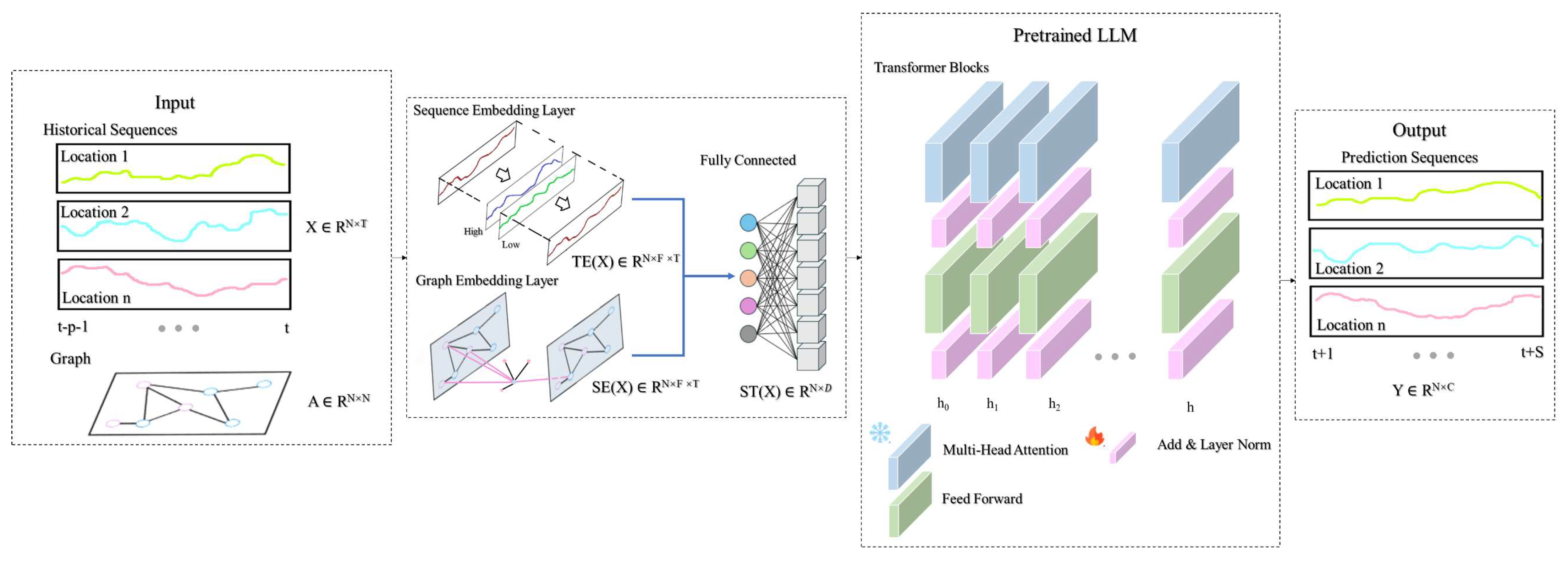
This paper designs an input embedding module to enable LLMs to better understand the spatiotemporal information contained in traffic flow data, and the overall structure of the prediction model is shown in Figure 1.

In the first module, SWT and LSTM process sequential traffic data, while GCN handles the adjacency matrix of the road network to extract spatiotemporal features separately. SWT is a time-shift invariant wavelet analysis method [30]. Herein, wavelet decomposition is performed along the traffic feature dimension of traffic flow data, generating a low-frequency approximation component (corresponding to the core temporal trend of a single feature) and a high-frequency detail component (corresponding to local fluctuations of a single feature). A convolution operation is then applied to adjust these two components: the trend is better aligned with the overall road network state, irrelevant sensor noise fluctuations are suppressed, and the trend of a single feature is integrated with those of other features (e.g., speed and density). For instance, the flow trend at a monitoring point is revised by incorporating its speed trend, which better conforms to the physical laws of traffic flow. Subsequently, in the time-series embedding layer, LSTM conducts sequence modeling on the SWT-processed reconstructed components to capture long-range temporal dependencies of traffic flow (e.g., the temporal correlation between morning and evening peaks), addressing the limitations that pure CNN cannot model long sequences and pure wavelet transform lacks sequence memory. The graph embedding layer takes the road network adjacency matrix as input and performs spatial convolution on the features of each traffic station via GCN to extract implicit spatial correlations and topological dependencies among stations. The structure of the sequences embedding layer is shown in Figure 2.

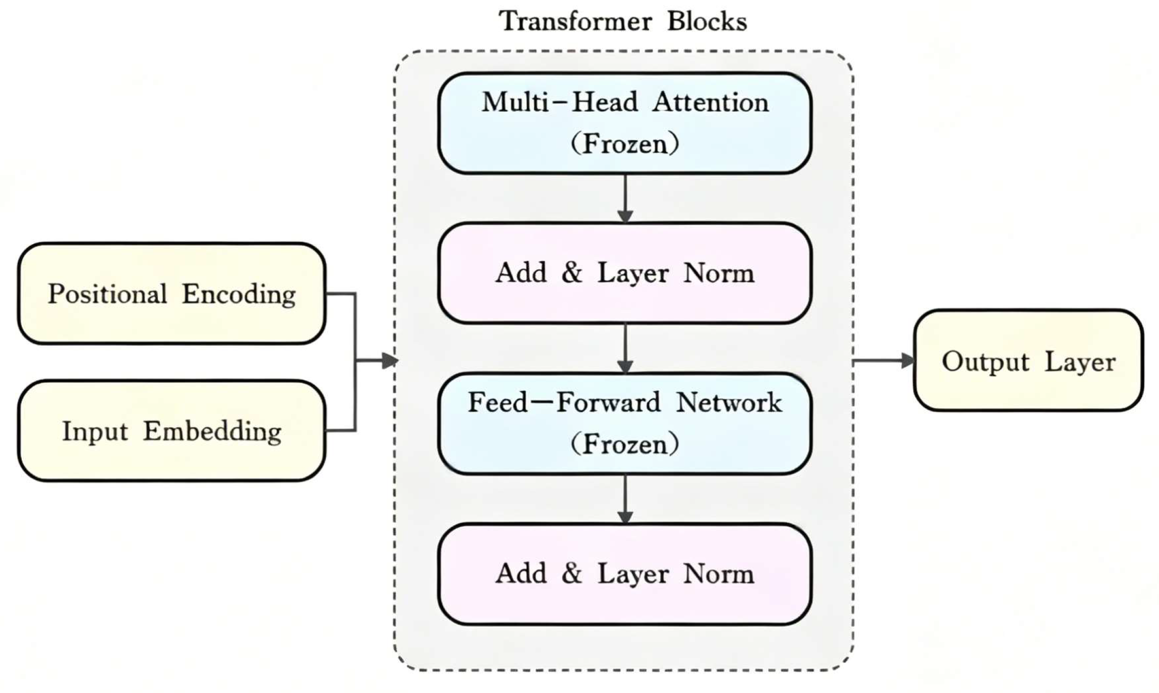
The FPT (Frozen Pretrained Transformer) framework follows the universal cross-modal frozen pretrained Transformer paradigm, whose core principle is to freeze all core parameters of the multi-head attention (MHA) layer and feed-forward network (FFN) in the pretrained Transformer, while only fine-tuning lightweight adaptation modules to achieve downstream task adaptation, preserving pretrained general knowledge and avoiding catastrophic forgetting [31]; the architecture is summarized in Figure 3. The temporal feature vector from time-series embedding and the spatial feature vector from graph embedding are fused and mapped via a linear layer into a sequence matching the FPT input dimension, enabling unified representation of traffic spatiotemporal features and FPT modal adaptation. FPT receives the fused spatiotemporal sequence and leverages its pre-learned universal sequence modeling capability and self-attention mechanism to capture global spatiotemporal dependencies in traffic spatiotemporal data.

By freezing the backbone layers and fine-tuning only a small number of parameters, FPT significantly reduces the number of learnable parameters, improving model performance and reducing training costs. Meanwhile, the spatiotemporal embedding layer extracts fine-grained local spatiotemporal features, while FPT performs coarse-grained global spatiotemporal correlation modeling, fully utilizing its universal sequence modeling and global mining capabilities learned from text pre-training. These two components complement each other to form a “local-global” dual-layer spatiotemporal modeling architecture, enhancing the model’s ability to represent traffic spatiotemporal data.

2.3. Spatiotemporal Embedding and Fusion

Graph Convolutional Networks (GCNs) perform convolution operations by leveraging the neighbor information of nodes, thereby achieving feature learning and representation learning on graphs. In this study, we designed a graph embedding layer based on GCNs to extract spatial information.

Given an undirected graph G = (V, E) and its feature matrix X ∈ R^{N × C}, the adjacency matrix A ∈ R^{N × N} is usually derived from the connectivity between nodes. The degree matrix D can be calculated by the formula $D_{ii}={\Sigma }_j{A}_{ij}$. Herein, N denotes the number of nodes, and C represents the dimension of the vector. Since each node should also take its own features into account, the original adjacency matrix ought to be updated to $\tilde{\mathrm{A}}$, with its corresponding degree matrix updated to $\tilde{\mathrm{D}}$. The specific calculation processes are shown:

$$\tilde{\mathrm{A}}=\mathrm{A}+\mathrm{I}$$

(2)

$${\tilde{D}}_{ii}={\Sigma }_j{\tilde{A}}_{ij}$$

(3)

Each node is made to consider the features of both its neighboring nodes and itself; these features are then linearly combined via a weight matrix to obtain new node representations, so as to update the information after node aggregation. The detailed calculation process is given:

$$h_s=ReLU({\tilde{D}}^{-{\displaystyle \frac{1}{2}}}\tilde{A}{\tilde{D}}^{-{\displaystyle \frac{1}{2}}}XW+b)$$

(4)

where $W$ is the learnable parameter matrix, $b$ is the learnable bias vector, and $ReLU(·)$ is the ReLU activation function.

Additionally, this study designs a sequence embedding layer based on the stationary wavelet transform and LSTM. The core feature of SWT is replacing the downsampling operation in the traditional Discrete Wavelet Transform (DWT) with filter upsampling, ensuring that the coefficient length at each decomposition layer remains consistent with the original signal, thereby eliminating the time-shift sensitivity of DWT. Let the original discrete signal be $s\in z{\mathrm{R}}^N$ with length N, and the number of decomposition layers be $J$ (satisfying $J\le {\mathrm{l}\mathrm{o}\mathrm{g}}_{2}N$). The original low-pass filter $\mathrm{h}=\left\{h_k\right\}$ and high-pass filter $\mathrm{g}=\left\{g_k\right\}$ satisfy orthogonality or biorthogonality conditions.

The filters used in the $j^{th}$ layer of SWT decomposition are obtained by upsampling the original filters: inserting $2^{j-1}-1$ zeros between every two adjacent elements of the original filter to match the signal length $N$. Mathematically, they are defined as:

$$h_j\left[k\right]=\left\{\begin{array}{ll}h\left[{\displaystyle \frac{k}{2^{j-1}}}\right]& \mathrm{if}k=m\cdot 2^{j-1}, 0\le m<L\\ 0& \mathrm{otherwise}\end{array}\right.$$

(5)

$$g_j\left[k\right]=\left\{\begin{array}{ll}g\left[{\displaystyle \frac{k}{2^{j-1}}}\right]& \mathrm{if}k=m\cdot 2^{j-1},0\le m<L\\ 0& \mathrm{otherwise}\end{array}\right.$$

(6)

where $L$ is the length of the original filter $\mathrm{h}$ (or $\mathrm{g}$), $h_j\left[k\right]$ and $g_j\left[k\right]$ are the upsampled low-pass and high-pass filters for the $j^{th}$ layer, respectively, with a length of $L\cdot 2^{j-1}$.

The $j^{th}$ layer decomposition of SWT is achieved by performing non-downsampling convolution on the approximation coefficients $A_{j-1}\left[n\right]$ of the ${j-1}^{th}$ layer, with the initial approximation coefficients $A_0\left[n\right]=s\left[n\right]$. If periodic extension is adopted for boundary handling (equivalent to circular convolution), the decomposition formulas are:

$$A_j\left[n\right]=\sum _k\hspace{0.17em}{h}_j\left[k\right]\cdot A_{j-1}\left[\left(n-k\right)\mathrm{m}\mathrm{o}\mathrm{d}N\right]$$

(7)

$$D_j\left[n\right]=\sum _k\hspace{0.17em}{g}_j\left[k\right]\cdot A_{j-1}\left[\left(n-k\right)\mathrm{m}\mathrm{o}\mathrm{d}N\right]$$

(8)

where $A_j\left[n\right]$ denotes the approximation coefficients of the $j^{th}$ layer, $D_j\left[n\right]$ denotes the detail coefficients of the $j^{th}$ layer, and the summation range covers the non-zero indices of $h_j\left[k\right]$ and $g_j\left[k\right]$. The term $(n-k)\mathrm{m}\mathrm{o}\mathrm{d}N$ realizes periodic extension of the signal to avoid index out-of-bounds during convolution. When zero extension or symmetric extension is used, $A_{j-1}\left[\left(n-k\right)\mathrm{m}\mathrm{o}\mathrm{d}N\right]$ can be replaced by $A_{j-1}(n-k)$ after corresponding boundary extension.

SWT reconstruction is realized by performing inverse filtering convolution on the coefficients of each layer. The dual filters ${\tilde{h}}_j$ and ${\tilde{g}}_j$ are used to weightily sum the approximation coefficients $A_j\left[n\right]$ and detail coefficients $D_j\left[n\right]$, and a normalization factor 1/2 is introduced to compensate for the energy accumulation caused by non-downsampling. When periodic extension is adopted, the reconstruction formula is:

$$A_{j-1}\left[n\right]={\displaystyle \frac{1}{2}}\left(\sum _k\hspace{0.17em}{\tilde{h}}_j\left[k\right]\cdot A_j\left[\left(n+k\right)\mathrm{m}\mathrm{o}\mathrm{d}N\right]+\sum _k\hspace{0.17em}{\tilde{g}}_j\left[k\right]\cdot D_j\left[\left(n+k\right)\mathrm{m}\mathrm{o}\mathrm{d}N\right]\right)$$

(9)

where ${\tilde{h}}_j$ and ${\tilde{g}}_j$ are the dual filters of $h_j$ and $g_j$, respectively: under orthogonal wavelet conditions, ${\tilde{h}}_j=h_j$ and ${\tilde{g}}_j=g_j$. The factor 1/2 is the key normalization term in SWT reconstruction, ensuring energy conservation and perfect signal reconstruction.

LSTM is a specialized recurrent neural network model that combines both long- and short-term memory, addressing the issues of gradient vanishing and gradient explosion. Its core is the Cell State, analogous to an information conveyor belt running through the entire time series. It maintains stable information transmission across time steps, enabling the network to memorize long-range information. At each time step, the Cell State is updated and transmits information under the joint control of the input, forget, and output gates. The first is the forget gate, which distinguishes between data to be retained or discarded using the following formula:

$$f_t={\sigma }_s(W_f{x}_t+W_f{h}_{t-1}+b_f)$$

(10)

where $x_t$ represents the input vector at the current time step and $h_{t-1}$ denotes the hidden state obtained at the previous time step. $W_f$ is the weight matrix of the forget gate, $b_f$ is the bias term of the forget gate and ${\sigma }_s(·)$ is the sigmoid activation function, with an output range of [0, 1], representing “how much information to retain”.

The second component is the input gate, which specifies the new information eligible for storage within the memory unit. The sigmoid layer confirms the values to be updated, yielding $i_t$, which is then processed through the $\mathrm{t}\mathrm{a}\mathrm{n}\mathrm{h}(·)$ layer to determine the data to be updated, generating the data vector $S_t$ and the new Cell State $C_t$:

$$i_t={\sigma }_s(W_i{x}_t+W_i{h}_{t-1}+b_i)$$

(11)

$$S_t=\mathrm{t}\mathrm{a}\mathrm{n}\mathrm{h}(W_c{x}_t+W_c{h}_{t-1}+b_c)$$

(12)

$$C_t=f_t\odot C_{t-1}+i_t{\odot S}_t$$

(13)

where $W_i$, $b_i$, $W_c$ and $b_c$ denote the weight matrices and bias vectors associated with the input gate, respectively. The $\mathrm{t}\mathrm{a}\mathrm{n}\mathrm{h}(·)$ is hyperbolic tangent (tanh) activation function and $\odot$ represents element-wise multiplication between corresponding elements.

The third is the output gate, which determines how much of the previous hidden state’s information $h_{t-1}$, the current input $x_t$, and previously obtained Cell State $C_t$ are passed to the next moment, and then performs the output:

$$o_t={\sigma }_s(W_o{x}_t+W_o{h}_{t-1}+b_o)$$

(14)

$$h_t=o_t\odot \mathrm{t}\mathrm{a}\mathrm{n}\mathrm{h}\left(C_t\right)$$

(15)

where $W_o$ and $b_o$ denote the weight matrix and bias vector of the output gate.

A core feature of FPT is freezing the Transformer’s core components, restricting the MHA layer and FFN from gradient updates during downstream training. By maintaining pretrained parameters, it preserves general representation capability and lays a foundation for cross-modal knowledge transfer. Its core constraint is:

$$\nabla {\theta }_{\mathrm{M}\mathrm{H}\mathrm{A}}=0,\nabla {\theta }_{\mathrm{F}\mathrm{F}\mathrm{N}}=0$$

(16)

where ${\theta }_{\mathrm{M}\mathrm{H}\mathrm{A}}$ is the parameter set of the MHA layer (including Q, K, V projection matrices and multi-head fusion matrix); ${\theta }_{\mathrm{F}\mathrm{F}\mathrm{N}}$ is the parameter set of the FFN (including linear transformation matrices $W_1$, $W_2$) and biases $b_1$, $b_2$ are the gradient operator.

Under parameter freezing, the MHA layer and FFN perform forward propagation to extract and enhance features. The frozen MHA layer captures input sequence global dependencies via parallel attention heads, with its forward propagation expressed as:

$${\mathrm{M}\mathrm{H}\mathrm{A}}_{\mathrm{f}\mathrm{r}\mathrm{e}\mathrm{e}\mathrm{z}\mathrm{c}}\left(x\right)=\mathrm{C}\mathrm{o}\mathrm{n}\mathrm{c}\mathrm{a}\mathrm{t}\left({\mathrm{H}\mathrm{e}\mathrm{a}\mathrm{d}}_1,{\mathrm{H}\mathrm{e}\mathrm{a}\mathrm{d}}_2,\dots ,{\mathrm{H}\mathrm{e}\mathrm{a}\mathrm{d}}_h\right)W_O$$

(17)

where $x$ is the adapted downstream input feature ($n\times d_{\mathrm{m}\mathrm{o}\mathrm{d}\mathrm{e}\mathrm{l}}$, $n$ = sequence length, $d_{\mathrm{m}\mathrm{o}\mathrm{d}\mathrm{e}\mathrm{l}}$ = model dimension); $\mathrm{h}$ = number of attention heads (fixed, typically 8 or 12); $W_O$ is the multi-head fusion matrix (${\theta }_{\mathrm{M}\mathrm{H}\mathrm{A}}$, frozen).

A single attention head (${\mathrm{H}\mathrm{e}\mathrm{a}\mathrm{d}}_i$) calculates normalized attention scores and feature weighting, with formulas:

$${\mathrm{H}\mathrm{e}\mathrm{a}\mathrm{d}}_i=\mathrm{S}\mathrm{o}\mathrm{f}\mathrm{t}\mathrm{m}\mathrm{a}\mathrm{x}\left({\displaystyle \frac{Q_i{K}_i^T}{\sqrt{d_k}}}\right)V_i$$

(18)

$$Q_i=x{W}_{Q_i},K_i=x{W}_{K_i},V_i=x{W}_{V_i}$$

(19)

where $d_k=d_{\mathrm{m}\mathrm{o}\mathrm{d}\mathrm{e}\mathrm{l}}/h$ (feature dimension of a single attention head); $Q_i$, $K_i$ and $V_i$ are Q, K, V projection matrices (${\theta }_{\mathrm{M}\mathrm{H}\mathrm{A}}$, frozen); $\sqrt{d_k}$ is a scaling factor to prevent Softmax saturation.

The frozen FFN performs nonlinear feature transformation, with its forward propagation formula:

$${\mathrm{F}\mathrm{F}\mathrm{N}}_{\mathrm{f}\mathrm{r}\mathrm{e}\mathrm{e}\mathrm{z}\mathrm{e}}\left(h_{\mathrm{M}\mathrm{H}\mathrm{A}}\right)=W_2\cdot \sigma \left(W_1\cdot h_{\mathrm{M}\mathrm{H}\mathrm{A}}+b_1\right)+b_2$$

(20)

where $h_{\mathrm{M}\mathrm{H}\mathrm{A}}$ is the MHA output (Equation (17)); $W_1$ maps $d_{\mathrm{m}\mathrm{o}\mathrm{d}\mathrm{e}\mathrm{l}}$ to ${4d}_{\mathrm{m}\mathrm{o}\mathrm{d}\mathrm{e}\mathrm{l}}$, and $W_2$ maps it back to $d_{\mathrm{m}\mathrm{o}\mathrm{d}\mathrm{e}\mathrm{l}}$; $W_1$, $W_2$, $b_1$, $b_2$ belong to ${\theta }_{\mathrm{F}\mathrm{F}\mathrm{N}}$ (frozen); $\sigma (·)$ is the activation function (ReLU or GELU) fixed during pretraining.

The complete FPT forward propagation, combined with lightweight adaptation modules (input adaptation, core feature extraction, output mapping), is expressed as:

$$x_{\mathrm{a}\mathrm{d}\mathrm{a}\mathrm{p}\mathrm{t}}=W_{\mathrm{e}\mathrm{m}\mathrm{b}\mathrm{e}\mathrm{d}}\cdot x_{\mathrm{r}\mathrm{a}\mathrm{w}}+b_{\mathrm{e}\mathrm{m}\mathrm{b}\mathrm{e}\mathrm{d}}$$

(21)

$$h_{\mathrm{M}\mathrm{H}\mathrm{A}}={\mathrm{M}\mathrm{H}\mathrm{A}}_{\mathrm{f}\mathrm{r}\mathrm{e}\mathrm{e}\mathrm{z}\mathrm{e}}\left(x_{\mathrm{a}\mathrm{d}\mathrm{a}\mathrm{p}\mathrm{t}}\right)$$

(22)

$$h_{\mathrm{F}\mathrm{F}\mathrm{N}}={\mathrm{F}\mathrm{F}\mathrm{N}}_{\mathrm{f}\mathrm{r}\mathrm{e}\mathrm{e}\mathrm{z}\mathrm{e}}\left(h_{\mathrm{M}\mathrm{H}\mathrm{A}}\right)$$

(23)

$$y_{\mathrm{o}\mathrm{u}\mathrm{t}}=W_{\mathrm{h}\mathrm{e}\mathrm{a}\mathrm{d}}\cdot h_{\mathrm{F}\mathrm{F}\mathrm{N}}+b_{\mathrm{h}\mathrm{e}\mathrm{a}\mathrm{d}}$$

(24)

where $x_{\mathrm{r}\mathrm{a}\mathrm{w}}$ is the original downstream input (e.g., time series, image patches); $W_{\mathrm{e}\mathrm{m}\mathrm{b}\mathrm{e}\mathrm{d}}$, $b_{\mathrm{e}\mathrm{m}\mathrm{b}\mathrm{e}\mathrm{d}}$ are trainable embedding parameters to map $x_{\mathrm{r}\mathrm{a}\mathrm{w}}$ to $d_{\mathrm{m}\mathrm{o}\mathrm{d}\mathrm{e}\mathrm{l}}$; Equations (22) and (23) are frozen core feature extraction with fixed parameters; $W_{\mathrm{h}\mathrm{e}\mathrm{a}\mathrm{d}}$, $b_{\mathrm{h}\mathrm{e}\mathrm{a}\mathrm{d}}$ are trainable output head parameters for downstream target space mapping. Only $W_{\mathrm{e}\mathrm{m}\mathrm{b}\mathrm{e}\mathrm{d}}$, $b_{\mathrm{e}\mathrm{m}\mathrm{b}\mathrm{e}\mathrm{d}}$, $W_{\mathrm{h}\mathrm{e}\mathrm{a}\mathrm{d}}$, $b_{\mathrm{h}\mathrm{e}\mathrm{a}\mathrm{d}}$ participate in gradient updates, reducing training cost and enabling efficient cross-modal and cross-task adaptation.

Finally, a linear transformation is performed through a fully connected layer to fuse graph embedding with sequence embedding, followed by normalization to project the temporal dimension of the fused features onto the embedding dimension D of LLMs, resulting in M∈R^N×F×D. The calculation is as follows:

$$M=LayerNorm\left(ReLU\right(Linear\left(h_t\right|\left|h_s\right)\left)\right)$$

(25)

where $LayerNorm(.)$ denotes layer normalization, $ReLU(.)$ is the activation function, $Linear(.)$ denotes the linear transformation layer that projects the input to dimension D, and || denotes concatenation.

3. Result

3.1. Dataset

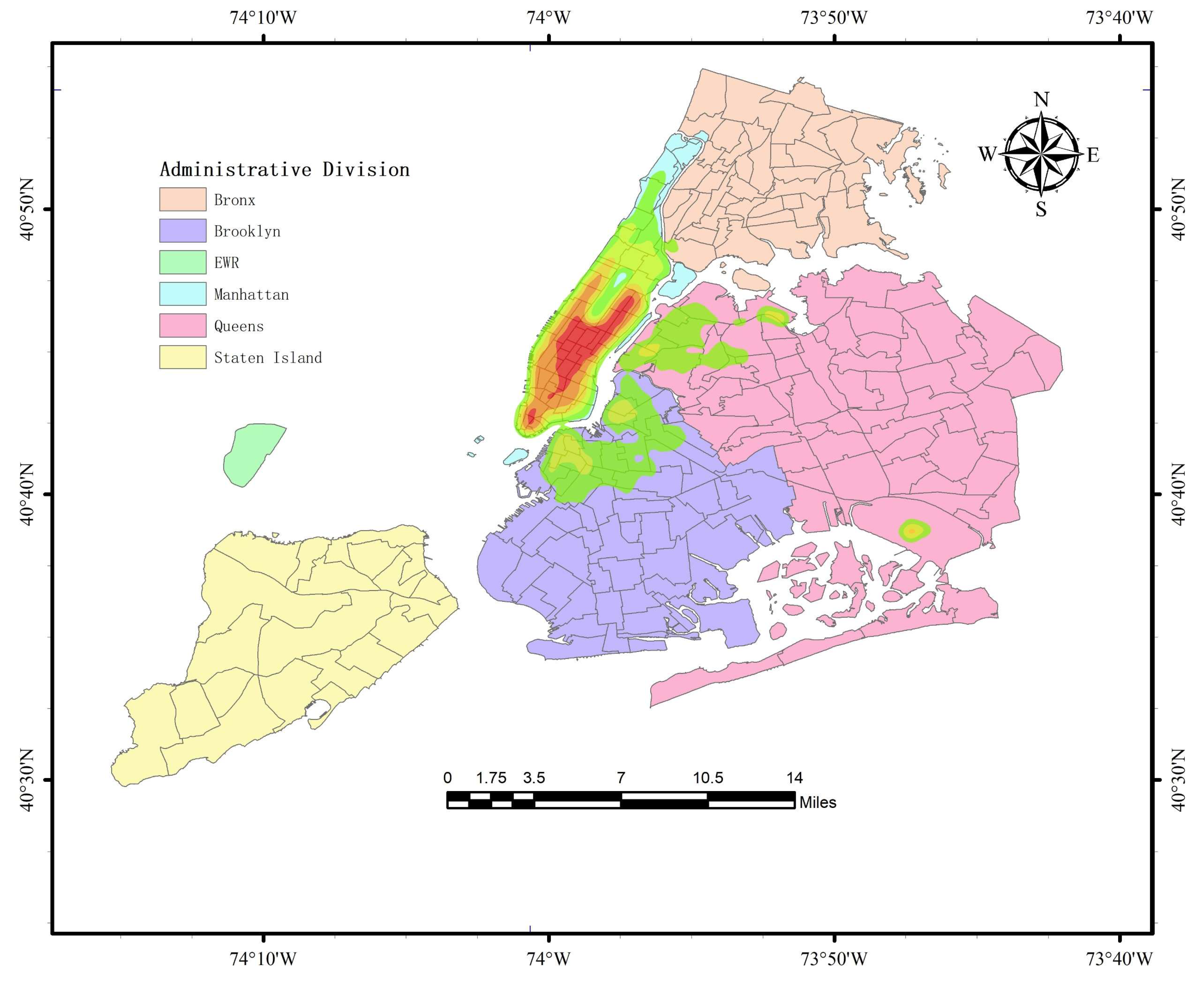
NYC Taxi: The New York City taxi dataset includes over 35 million taxi trips in New York City, systematically divided into 266 virtual stations. Over the three-month period from 1 April to 30 June 2016, it includes 4368 time steps. Spatial uniform sampling was performed on the NYC Taxi dataset using the minimum distance thinning method, and kernel density estimation was conducted at the geographic scale of New York City. The results are shown in Figure 4.

CH Bike: The CH Bike dataset consists of approximately 2.6 million Citi Bike orders, reflecting the usage of the bike-sharing system during the same period as the New York taxi dataset, from 1 April to 30 June 2016. After filtering out stations with fewer orders, the focus was on the 250 most frequently used stations. Aligned temporally with the New York City Taxi dataset, the dataset comprises 4368 time steps, where each step denotes a 30 min time window.

3.2. Experimental Setup

Experimental implementation relied on the Python 3.8.19 and PyTorch 2.4.1, with the network architecture running on an NVIDIA (Santa Clara, CA, USA) GeForce RTX 4070Ti graphics processing unit. The dataset was split into training, validation, and test partitions following a 6:2:2 ratio. In the training process, the mean square error (MSE) was selected as the loss function, and parameter updates were performed using the Ranger optimizer. The specific experimental parameters are shown in

Table 1. Experimental hyperparameters.

Hyperparameter	Value
Epochs	500
Learning rate	0.01
Dropout	0.001
Weight decay	0.0001
Channels	64
Batch size	64
Output lengths	12
Es patience	50

(Es patience: quit if no improvement after this many iterations).

3.3. Evaluation Metrics

To assess the performance of the model, this paper employs four widely adopted evaluation metrics: Mean Absolute Error ($\mathrm{M}\mathrm{A}\mathrm{E}$), Mean Absolute Percentage Error ($\mathrm{M}\mathrm{A}\mathrm{P}\mathrm{E}$), Root Mean Square Error ($\mathrm{R}\mathrm{M}\mathrm{S}\mathrm{E}$), and Weighted Absolute Percentage Error ($\mathrm{W}\mathrm{A}\mathrm{P}\mathrm{E}$).

$$\mathrm{M}\mathrm{A}\mathrm{E}={\displaystyle \frac{1}{m}}\sum _{i=1}^m\hspace{0.17em}\left|{\widehat{\mathrm{Y}}}_i-{\mathrm{Y}}_i\right|$$

(26)

$$\mathrm{M}\mathrm{A}\mathrm{P}\mathrm{E}={\displaystyle \frac{100\%}{m}}\sum _{i=1}^m\hspace{0.17em}\left|{\displaystyle \frac{{\widehat{\mathrm{Y}}}_i-{\mathrm{Y}}_i}{{\mathrm{Y}}_i}}\right|$$

(27)

$$\mathrm{R}\mathrm{M}\mathrm{S}\mathrm{E}=\sqrt{{\displaystyle \frac{1}{m}}\sum _{i=1}^m\hspace{0.17em}{\left({\widehat{\mathrm{Y}}}_i-{\mathrm{Y}}_i\right)}^2}$$

(28)

$$\mathrm{W}\mathrm{A}\mathrm{P}\mathrm{E}={\displaystyle \frac{\sum _{i=1}^m\hspace{0.17em}\left|{\widehat{\mathrm{Y}}}_i-{\mathrm{Y}}_i\right|}{\sum _{i=1}^m\hspace{0.17em}\left|{\mathrm{Y}}_i\right|}}\times 100\%$$

(29)

3.4. Comparison of Experimental Results

This study compares the WGLLM with the following six baseline models, with results shown in

Table 2. Prediction performance metrics of various baseline models and WGLLM on different datasets.

Dataset	NYCTaxi Pick-Up				NYCTaxi Drop-Off				CHBike Pick-Up				CHBike Drop-Off
Metric	MAE	RMSE	MAPE	WAPE	MAE	RMSE	MAPE	WAPE	MAE	RMSE	MAPE	WAPE	MAE	RMSE	MAPE	WAPE
ASTGCN	7.43	13.84	47.96%	28.04%	6.98	14.70	45.48%	26.60%	2.76	4.45	64.23%	55.71%	2.79	4.20	69.88%	56.49%
ASTGNN	5.90	10.71	40.15%	22.32%	6.28	12.00	49.78%	23.97%	2.37	3.67	60.08%	47.81%	2.24	3.35	57.21%	45.27%
GMAN	5.43	9.47	34.39%	20.42%	5.09	8.95	35.00%	19.33%	2.20	3.35	57.34%	44.06%	2.09	3.00	54.82%	42.00%
STSGCN	6.19	11.14	39.67%	25.37%	5.62	10.21	37.92%	22.59%	2.36	3.73	58.17%	50.09%	2.73	4.50	57.89%	54.10%
AGCRN	5.79	10.11	40.40%	21.93%	5.45	9.56	40.67%	20.81%	2.16	3.46	56.35%	43.69%	2.06	3.19	51.91%	41.78%
STGNCDE	6.24	11.25	43.20%	23.46%	5.38	9.74	40.45%	21.37%	2.15	3.97	55.49%	61.38%	2.28	3.42	60.96%	46.06%
OFA	5.81	10.40	36.65%	22.00%	5.58	10.12	37.37%	21.36%	2.04	3.23	53.55%	41.70%	1.94	2.91	50.68%	39.29%
GATGPT	5.90	10.53	37.83%	22.39%	5.64	10.33	37.36%	21.60%	2.05	3.23	53.54%	41.70%	1.93	2.88	50.20%	39.04%
WGLLM	5.33	9.43	36.01%	20.18%	5.04	9.23	33.03%	19.25%	2.02	3.14	52.91%	40.76%	1.92	2.86	50.80%	38.98%

(All baseline models relied on Python 3.8.19 and PyTorch 2.4.1.):

• AGCRN [32]: a graph convolutional recurrent network with adaptive mechanisms that integrates node-wise learning and the deduction of inter-traffic-sequence mutual dependencies.
• STG-NCDE [33]: this method proposes a graph neural network-driven differential equation for processing sequence data.
• ASTGCN: a spatiotemporal graph convolutional framework incorporating attention mechanisms to predict traffic conditions.
• GMAN [34]: a prediction model with attention mechanisms based on the encoder–decoder framework.
• ASTGN [35]: a model integrated with attention mechanisms for learning the dynamics and heterogeneity inherent in traffic data.
• STSGCN: a model adopting a spatiotemporal synchronous modeling mechanism: it captures local spatiotemporal correlations and designs multiple time-period-specific modules to model the heterogeneity of local spatiotemporal graphs.
• OFA [29]: constructs a unified framework by freezing the core layers of pre-trained language/vision models, achieving state-of-the-art or comparable performance across diverse time-series analysis tasks including classification, long- and short-term prediction, imputation, anomaly detection, and few-shot/zero-shot learning.
• GATGPT [36]: integrates a graph attention network (GAT) with a pre-trained large language model for spatiotemporal data imputation, enabling joint modeling of non-Euclidean spatial structural features and long-range sequential dependencies.

Based on the experimental findings, the proposed model achieved optimal performance metrics across all four datasets, outperforming the remaining baseline models by a notable margin. Among these baselines, ASTGCN yielded the least favorable comprehensive performance, which is likely due to its dependence on a hybrid of graph convolution and temporal convolution for spatiotemporal feature extraction. Such a localized convolutional approach falls short of satisfactory outcomes when addressing complex spatiotemporal dynamics, such as spatiotemporal dependencies within long sequences. In contrast, ASTGNN employs an attention mechanism to explore spatiotemporal patterns within the data, adaptively focusing on critical information across diverse time steps and spatial locations. This endows it with a superior capacity to extract non-local spatiotemporal features of greater global significance, thereby outperforming the ASTGCN by a notable degree. The STSGCN captures local spatiotemporal correlations via building local spatiotemporal graphs and spatiotemporal synchronous graph convolution modules. Although it accounts for the spatiotemporal neighborhood information of nodes, its capacity to model complex dynamic spatiotemporal correlations remains relatively constrained. In contrast, GMAN incorporates a spatiotemporal attention mechanism: spatial attention dynamically captures inter-node spatial dependencies, adaptively quantifying the importance of each node to others; temporal attention addresses nonlinear temporal correlations, effectively capturing complex relationships among traffic conditions across varying time steps. Moreover, via a gated fusion mechanism, the GMAN dynamically modulates the contributions of spatial and temporal attention, balancing their influence on model outputs.

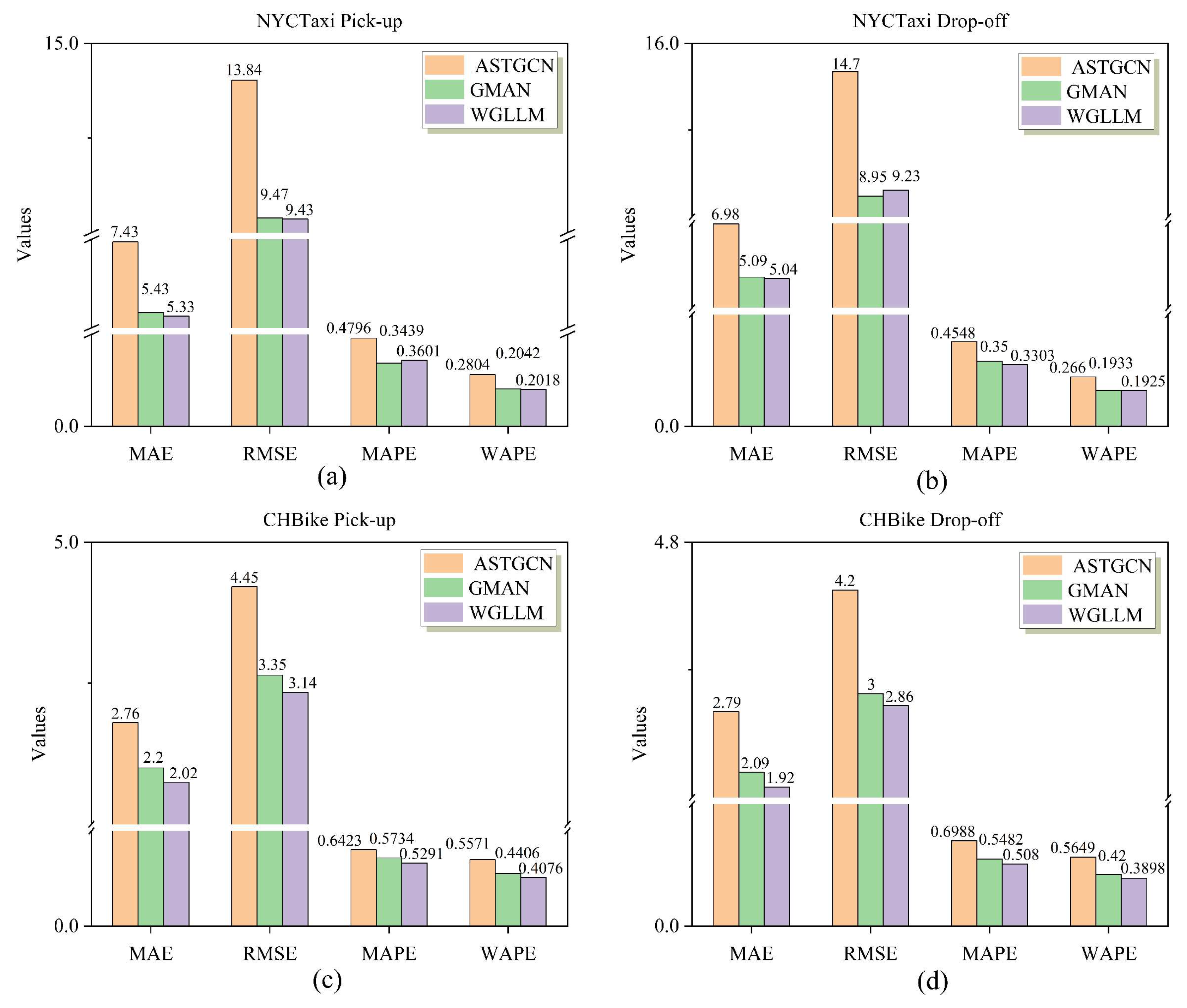
Among the six baseline models, ASTGCN yielded the least favorable comprehensive metrics, whereas GMAN attained the optimal overall performance. Figure 5 illustrates the performance metrics of the ASTGCN, GMAN, and WGLLM across diverse datasets. Relative to GMAN, our proposed WGLLM achieved a notable performance enhancement on the CHBike dataset: MAE decreased by 8.2% and 8.1%, RMSE by 6.3% and 4.7%, MAPE by 7.7% and 7.3%, and WAPE by 7.5% and 7.2%. Such discrepancies may arise from the inherent limitations of traditional attention mechanisms. GNN-based models (ASTGNN and AGCRN) exhibited competitive performance in specific metrics yet failed to surpass the WGLLM. This suggests that the temporal analytical capacities of GNN constrain its overall performance. In conclusion, the proposed WGLLM demonstrates superior performance on traffic flow datasets and enables effective modeling of traffic flow data.

3.5. Ablation Experiments

With the aim of verifying the effectiveness of each constituent component in the proposed model, four variants were designed, and ablation experiments were conducted on both the CHBike Pick-up and CHBike Drop-off datasets. The results are presented in

Table 3. Predictive performance metrics (MAE, RMSE, MAPE (%), and WAPE (%)) of each ablation variant model and WGLLM.

Dataset	CHBike Pick-Up				CHBike Drop-Off
Metric	MAE	RMSE	MAPE	WAPE	MAE	RMSE	MAPE	WAPE
wo-ST	2.20	3.35	57.34%	44.06%	2.09	3.00	54.82%	42.00%
wo-TE	2.36	3.73	58.17%	50.09%	2.73	4.50	57.89%	54.10%
wo-SE	2.16	3.46	56.35%	43.69%	2.06	3.19	51.91%	41.78%
wo-GP	2.15	3.97	55.49%	61.38%	2.28	3.42	60.96%	46.06%
WGLLM	2.02	3.14	52.91%	40.76%	1.92	2.86	50.80%	38.98%

:

(1)

”wo-ST”: A variant of WG-LLM with the spatiotemporal embedding module removed.

(2)

”wo-TE”: A variant of WG-LLM with the temporal embedding module removed.

(3)

”wo-SE”: A variant of WG-LLM with the spatial embedding module removed.

(4)

”wo-GP”: A variant of WG-LLM with the large language model module removed.

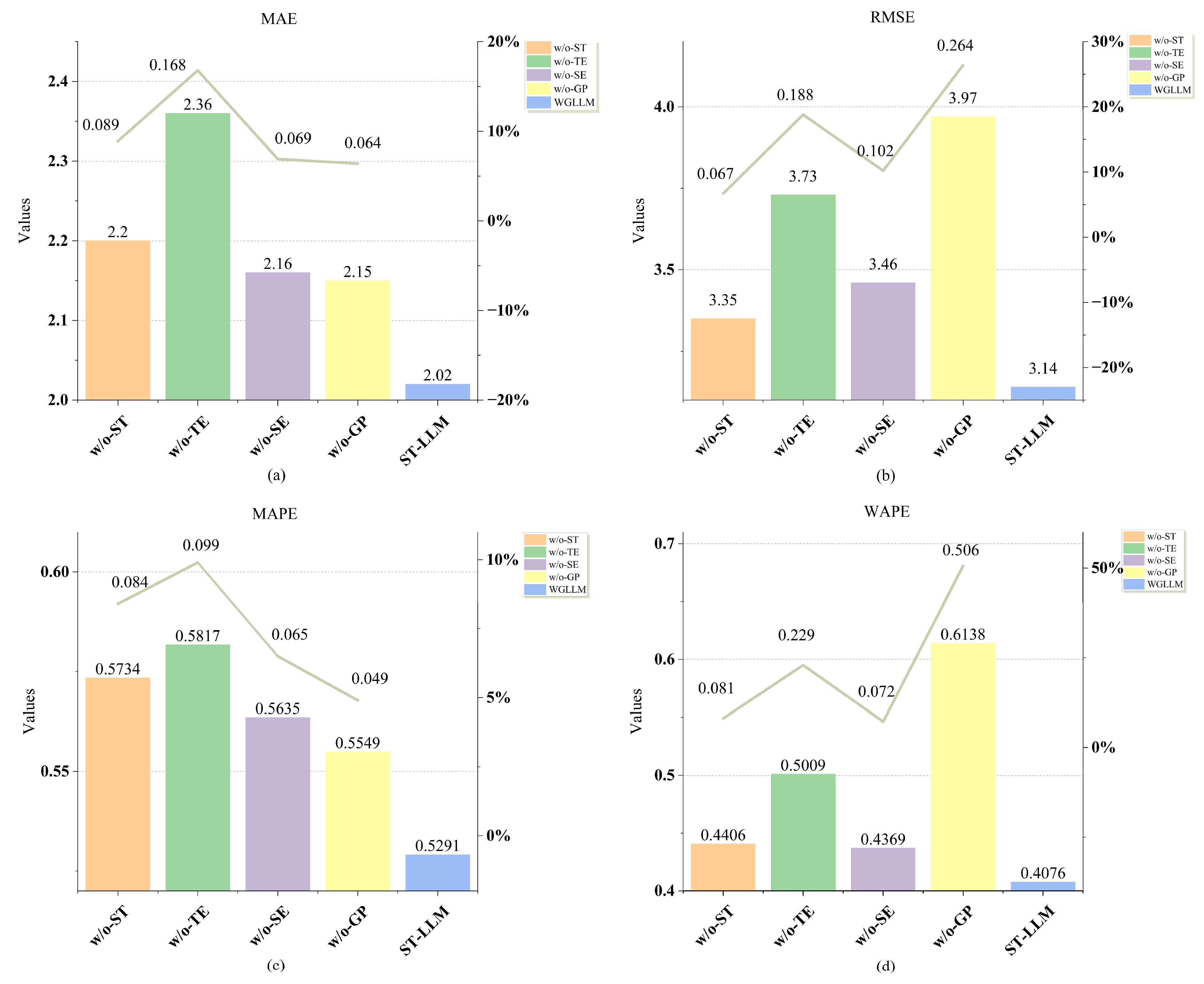
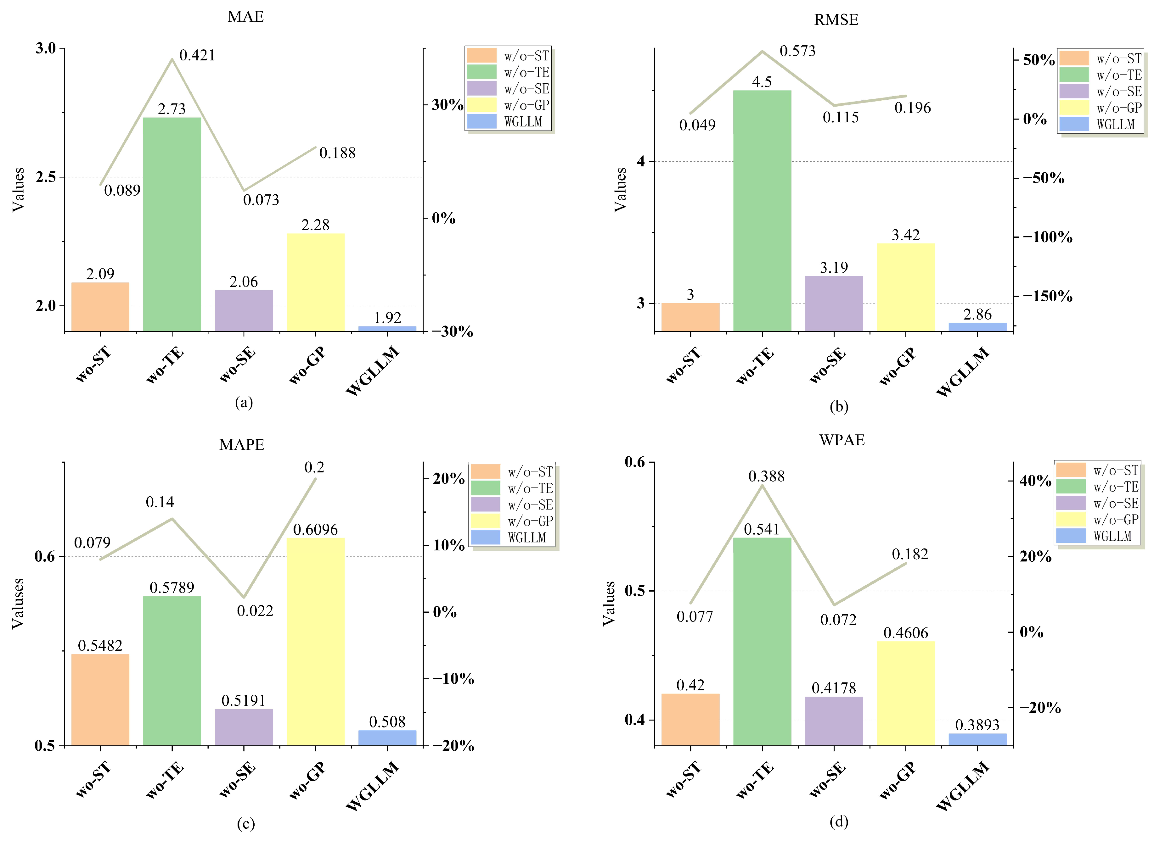
Figure 6 and Figure 7 depict the predictive performance of the WGLLM and its degraded variants on the CHBike dataset (average values of the evaluation metrics for 12-step predictions). Experimental results demonstrate that the original framework achieves the highest accuracy, validating that the temporal embedding layer, spatial embedding layer, spatiotemporal fusion module, and large language model module all exert a positive influence on the framework’s predictive performance.

Notably, the model excluding the temporal embedding layer exhibited the poorest predictive performance, with the MAE increasing by 16.83% and 42.18% respectively. This finding underscores the temporal embedding layer’s most prominent influence. The present study argues that, given the intrinsic time-series property of traffic flow data, the inherent characteristics of the time sequence are of paramount importance. The temporal embedding layer, which comprises a stationary wavelet transform and LSTM, effectively extracts sequence-specific features, rendering this module indispensable.

The model lacking the spatial embedding layer exhibited elevated values across all metrics, indicating that the adoption of GCN enables the efficient extraction of spatial features from traffic data, thereby boosting the accuracy of traffic prediction.

The model excluding the large language model module displayed differential increments across all metrics. On the CHBike Pick-up dataset, the RMSE and WAPE increased by 26.43% and 50.59%, respectively, far exceeding those of the other two metrics. Given that RMSEs amplify the impact of larger deviations and WAPE reflects the prediction bias at the overall traffic flow scale, this suggests the presence of significant “extreme fluctuations” or “key information in high-flow intervals” within the CHBike Pick-up dataset. In the CHBike Drop-off dataset, a marked increase in MAPE indicates that the dataset encompasses a multitude of “low-flow interval samples” that substantially influence the overall error. Accordingly, this study concludes that this module is endowed with the capacity to “adaptively process key features across different flow intervals” and is pivotal in balancing the learning of high- and low-flow samples, as well as capturing diverse flow patterns (including extreme fluctuations and subtle variations).

4. Discussion

Given the inherent complexity and dynamic nature of traffic flow, accurate prediction and analysis necessitate a profound understanding of spatiotemporal evolution patterns. However, in deep learning-based traffic flow prediction research, the distribution shift problem is prevalent, resulting in suboptimal generalization capability when processing data with heterogeneous spatiotemporal distributions. To mitigate this challenge, numerous approaches have been proposed in recent years, including domain adaptation, domain generalization, and data augmentation techniques [37,38,39,40]. Additionally, by virtue of their robust few-shot learning capacities and cross-modal knowledge transfer capabilities [31], LLMs can be fine-tuned efficiently to adapt to downstream tasks with distinct characteristics efficiently and cost-effectively, significantly expanding their functionality and enhancing their adaptability to practical requirements.

The advancement of deep learning technologies has propelled traffic flow prediction into the stage of spatiotemporal coupling modeling, giving rise to two major branches: convolutional/recurrent neural network-based models and graph neural network-based models. Models such as CNN-LSTM and ConvLSTM capture grid-based spatial features via convolution operations and exploit temporal dependencies with LSTM, yet struggle to adapt to the non-Euclidean spatial structure of traffic road networks [41]. Graph neural network models including GCN, STGCN, and DCRNN abstract the traffic road network as a graph structure, enabling the extraction of local features in non-Euclidean space, and have become the mainstream framework for current traffic flow prediction. However, such models are prone to over-smoothing and fail to capture cross-regional global spatiotemporal dependencies [42]. In recent years, large language models (LLMs) have been introduced into the field of traffic flow prediction, achieving global sequence modeling relying on pre-trained knowledge. Nevertheless, standalone LLMs often neglect fine-grained spatiotemporal features of traffic flow, leading to insufficient adaptability.

This paper proposes a traffic flow prediction model, WGLLM, positioned as a deep learning architecture that integrates the global modeling capability of large pre-trained models with dedicated spatiotemporal feature extraction modules. It fits into the evolutionary chain of traffic flow prediction from local spatiotemporal dependency modeling to collaborative global-local spatiotemporal feature modeling. With FPT as the core backbone, the model incorporates an SWT-LSTM multi-scale temporal feature extraction module and a GCN spatial feature extraction module. It not only inherits the adaptability of graph neural networks to the non-Euclidean structure of traffic road networks, but also breaks through the limitation of traditional deep learning models that can only capture local spatiotemporal dependencies. Meanwhile, it compensates for the deficiency of pure LLMs in characterizing fine-grained spatiotemporal features, constituting a technical paradigm bridging traditional deep learning spatiotemporal models and LLM-based traffic prediction models. Furthermore, the decoupled three-layer architecture designed in the model—spatiotemporal feature extraction, fusion, and global modeling—realizes collaborative modeling between fine-grained local spatiotemporal feature extraction and global spatiotemporal correlation mining. This enriches the theory of representation and modeling of traffic flow spatiotemporal features and provides a theoretical framework for the integrated application of large pre-trained models and traffic flow spatiotemporal feature extraction modules.

In engineering practice, traffic flow prediction models face three core pain points: weak cross-scenario generalization ability, high training costs, and low prediction accuracy in abnormal scenarios [22]. Traditional deep learning models rely on extensive local data for training, and their parameters exhibit strong scenario dependence; thus, retraining is required for cross-city or cross-traffic-mode migration, resulting in high application costs. Standalone LLMs have an enormous number of parameters, leading to high training and inference costs. Moreover, their insufficient characterization of fine-grained spatiotemporal features of traffic flow causes a sharp drop in prediction accuracy under abnormal conditions such as sudden traffic events [43,44]. The model proposed in this paper is complementary and optimized based on existing research. Leveraging the universal pre-trained knowledge of FPT, the model only needs fine-tuning of the input embedding layer parameters to rapidly adapt to traffic flow prediction tasks in different cities and across various traffic modes. This significantly reduces the computational costs of training and inference, making it suitable for real-time prediction demands in engineering applications.

The core engineering value of traffic flow prediction lies in providing a quantitative spatiotemporal demand basis for traffic demand management and urban traffic planning, addressing the core pain point of “experience-based decision-making and static schemes adapting to dynamic demands” in traditional management and planning [22]. The WGLLM traffic flow prediction model proposed in this paper, relying on three technical advantages—fine-grained prediction accuracy, global spatiotemporal characterization capability, and cross-scenario transferability—can be deeply applied throughout the entire process of urban traffic operation and management, and provide dynamic and accurate demand data support for meso-micro traffic planning, which is consistent with the development demands of modern intelligent transportation systems for “intelligent management, scientific planning, and efficient resource utilization” [45]. Specifically, aiming at the prominent crux of inefficient allocation of traffic resources in urban traffic operation—i.e., the mismatch between multi-mode traffic resource allocation (such as public transport, taxis, and shared bikes) and actual demand due to the lack of accurate characterization of spatiotemporal distribution of traffic flow—the model’s fine-grained spatiotemporal prediction capability and high adaptability can provide quantitative guidance. Based on the predicted results of road segment traffic flow, it can optimize lane function division and temporary parking area settings to realize efficient utilization of road resources. Its characteristics of low computational cost and fast inference speed can also support real-time updates of allocation schemes, significantly reducing operation and management costs. Meanwhile, addressing the problem that traditional meso-micro traffic planning relies on static data and has insufficient adaptability to dynamic demands, the model can accurately capture the global spatiotemporal dependence characteristics of traffic flow, provide dynamic and global traffic flow demand data for road network optimization, public transport network planning, traffic hub layout and other work, offer support for the coordinated planning of urban comprehensive traffic networks, help realize the integrated planning of “roads, networks, and hubs”, and improve the implementation and long-term applicability of planning schemes.

In summary, this paper proposes the WGLLM for traffic flow prediction, which bridges traditional deep learning methods and large language models. It delivers key contributions to traffic flow prediction modeling in terms of theory, methodology, and practical application. Furthermore, the model can support traffic demand management and planning, promote their intelligent and refined upgrading, and provide important technical support for the construction of intelligent transportation systems.

5. Conclusions

To address the challenge of urban traffic flow prediction, this study introduces a spatiotemporal large language model (LLM). The model integrates two core modules: a temporal feature extraction module leveraging stationary wavelet transform and LSTM, and a spatial feature extraction module drawing on GCN. These extracted features are subsequently fused and embedded through fully connected layers, allowing the LLMs to accommodate time-series data characteristics and capture global spatiotemporal dependencies in traffic prediction. Extensive experiments on the CHBike and NYCTaxi datasets revealed the proposed LLMs-integrated prediction model for traffic flow outperforms mainstream baseline models with superior performance. Furthermore, ablation experiments confirmed the efficacy of the temporal embedding layer, spatial embedding layer, spatiotemporal fusion module, and large language model module, with the SWT-LSTM-based temporal embedding layer exerting the most significant influence on model accuracy.

By embedding spatiotemporally fused traffic data into the LLM, the WGLLM exhibits promising potential in adapting large language models to traffic flow prediction. Given that real-world road network traffic flow is shaped by numerous external factors, future research should focus on integrating external variables, including traffic accidents and weather conditions, into the prediction framework. Furthermore, we plan to construct knowledge graphs based on physical locations (e.g., commercial districts, hospitals, and schools) adjacent to road segments, which are zones prone to high traffic generation, and utilize these graphs as input data. Such enhancements are intended to improve prediction accuracy and foster greater synergy across associated industrial chains.

References

1. Ammar, H.; Yılmaz, Y. Deep reinforcement learning for intelligent transportation systems: A survey. IEEE Trans. Intell. Transp. Syst. 2022, 23, 11–32. [Google Scholar]
2. Yin, X.; Wu, G.; Wei, J.; Shen, Y.; Qi, H.; Yin, B. Deep learning on traffic prediction: Methods, analysis, and future directions. IEEE Trans. Intell. Transp. Syst. 2021, 23, 4927–4943. [Google Scholar] [CrossRef]
3. Liu, G.; Long, W.; Wang, J.; Gao, P. Improving the throughput of transportation networks with a time-optimization routing strategy. Int. J. Geogr. Inf. Sci. 2018, 32, 1815–1836. [Google Scholar] [CrossRef]
4. Du, Y.; Liu, G.; Jiang, Y.; Cai, S.; He, J. Adaptive congestion index-based A* algorithm for dynamic vehicle path planning optimization. Phys. A: Stat. Mech. Its Appl. 2025, 672, 130702. [Google Scholar] [CrossRef]
5. Du, Y.; Liu, G.; Jiang, Y.; Si, Z.; He, J. Analysis of urban traffic flow characteristics considering driving behavior. Transp. Plan. Technol. 2025, 1–19. [Google Scholar] [CrossRef]
6. Tian, T.; Liu, G.; Hu, X.; Bian, D. Traffic behavior analysis of the urban expressway ramp based on continuous cellular automata. Phys. A Stat. Mech. Its Appl. 2024, 633, 129418. [Google Scholar] [CrossRef]
7. Cai, S.; Liu, G.; He, J.; Du, Y.; Si, Z.; Jiang, Y. Temporal-Spatial Traffic Flow Prediction Model Based on Prompt Learning. ISPRS Int. J. Geo-Inf. 2025, 14, 11. [Google Scholar] [CrossRef]
8. Williams, B.M.; Durvasula, P.K.; Brown, D.E. Urban Freeway Traffic Flow Prediction: Application of Seasonal Autoregressive Integrated Moving Average and Exponential Smoothing Models. Transp. Res. Rec. 1998, 1664, 132–141. [Google Scholar] [CrossRef]
9. Ahmed, M.S.; Cook, A.R. Analysis of Freeway Traffic Time-Series Data by Using Box-Jenkins Techniques. Transp. Res. Rec. 1979, 733, 1–9. [Google Scholar]
10. Williams, B.M. Multivariate Vehicular Traffic Flow Prediction: Evaluation of ARIMAX Modeling. Transp. Res. Rec. 2001, 1776, 194–200. [Google Scholar] [CrossRef]
11. Okutani, I.; Stephanedes, Y.J. Dynamic Prediction of Traffic Volume through Kalman Filtering Theory. Transp. Res. Part B Methodol. 1984, 18, 1–11. [Google Scholar] [CrossRef]
12. Davis, G.A.; Nihan, N.L. Nonparametric Regression and Short-Term Freeway Traffic Forecasting. J. Transp. Eng. 1991, 117, 178–188. [Google Scholar] [CrossRef]
13. Vanajakshi, L.; Rilett, L.R. A comparison of the performance of artificial neural networks and support vector machines for the prediction of traffic speed. In Proceedings of the IEEE Intelligent Vehicles Symposium, Parma, Italy, 14–17 June 2004; pp. 194–199. [Google Scholar]
14. Wu, C.; Ho, J.; Lee, D. Travel-Time Prediction with Support Vector Regression. IEEE Trans. Intell. Transp. Syst. 2004, 5, 276–281. [Google Scholar] [CrossRef]
15. Wang, Y.; Gao, Z.; Long, M.; Wang, J.; Philip, S.Y. PredRNN++: Towards A Resolution of the Deep-in-Time Dilemma in Spatiotemporal Predictive Learning. In Proceedings of the International Conference on Machine Learning, Stockholm, Sweden, 10–15 July 2018; pp. 5123–5132. [Google Scholar]
16. Lin, Z.; Li, M.; Zheng, Z.; Cheng, Y.; Yuan, C. Self-attention convlstm for spatiotemporal prediction. Proc. AAAI Conf. Artif. Intell. 2020, 34, 11531–11538. [Google Scholar] [CrossRef]
17. Zhao, Z.; Chen, W.; Wu, X.; Chen, P.C.; Liu, J. LSTM network: A deep learning approach for short-term traffic forecast. IET Intell. Transp. Syst. 2017, 11, 68–75. [Google Scholar] [CrossRef]
18. Zhang, Q.; Zhou, L.; Su, Y.; Xia, H.; Xu, B. Gated Recurrent Unit Embedded with Dual Spatial Convolution for Long-Term Traffic Flow Prediction. ISPRS Int. J. Geo-Inf. 2023, 12, 366. [Google Scholar] [CrossRef]
19. Ranjan, N.; Bhandari, S.; Zhao, H.; Kim, H.; Khan, P. City-wide traffic congestion prediction based on CNN, LSTM and transpose CNN. IEEE Access 2020, 8, 81606–81620. [Google Scholar] [CrossRef]
20. Zhang, W.; Yu, Y.; Qi, Y.; Shu, F.; Wang, Y. Short-term traffic flow prediction based on spatio-temporal analysis and CNN deep learning. Transp. A Transp. Sci. 2019, 15, 1688–1711. [Google Scholar] [CrossRef]
21. Zhao, L.; Song, Y.; Zhang, C.; Liu, Y.; Wang, P.; Lin, T.; Deng, M.; Li, H. T-GCN: A Temporal Graph Convolutional Network for Traffic Prediction. IEEE Trans. Intell. Transp. Syst. 2020, 21, 3848–3858. [Google Scholar] [CrossRef]
22. Yu, B.; Yin, H.; Zhu, Z. Spatio-temporal graph convolutional networks: A deep learning framework for traffic forecasting. In Proceedings of the 27th International Joint Conferences on Artificial Intelligence, Stockholm, Sweden, 15–21 August 2018; pp. 3634–3640. [Google Scholar] [CrossRef]
23. Guo, S.; Lin, Y.; Feng, N.; Song, C.; Wan, H. Attention based spatial-temporal graph convolutional networks for traffic flow forecasting. In Proceedings of the AAAI Conference on Artificial Intelligence, Honolulu, HI, USA, 27 January–1 February 2019; Volume 33, pp. 922–929. [Google Scholar] [CrossRef]
24. Song, C.; Lin, Y.; Guo, S.; Wan, H. Spatial-temporal synchronous graph convolutional networks: A new framework for spatial-temporal network data forecasting. Proc. AAAI Conf. Artif. Intell. 2020, 34, 914–921. [Google Scholar] [CrossRef]
25. Hu, E.; Shen, Y.; Wallis, P.; Allen-Zhu, Z.; Li, Y.; Wang, S.; Wang, L.; Chen, W. LoRA: Low-Rank Adaptation of Large Language Models. In Proceedings of the International Conference on Learning Representations, Online, 25–29 April 2022. [Google Scholar]
26. Radford, A.; Wu, J.; Child, R.; Luan, D.; Amodei, D.; Sutskever, I. Language models are unsupervised multitask learners. OpenAI Blog 2019, 1, 8. [Google Scholar]
27. Brown, T.; Mann, B.; Ryder, N.; Subbiah, M.; Kaplan, J.; Djariwal, P.; Neelakantan, A.; Shyam, P.; Sastry, G.; Askell, A.; et al. Language models are few-shot learners. In Proceedings of the 34th International Conference on Neural Information Processing Systems, Vancouver, BC, Canada, 6–12 December 2020; pp. 1877–1901. [Google Scholar]
28. Achiam, J.; Adler, S.; Agarwal, S.; Ahmad, L.; Akkaya, I.; Aleman, F.L.; Almeida, D.; Altenschmidt, J.; Altman, S.; Anadkat, S.; et al. Gpt-4 Technical Report. arXiv 2023, arXiv:2303.08774. [Google Scholar] [CrossRef]
29. Zhou, T.; Niu, P.; Wang, X.; Sun, L.; Jin, R. One fits all: Power general time series analysis by pretrained lm. In Proceedings of the 37th Conference on Neural Information Processing Systems, New Orleans, LA, USA, 10–16 December 2024; pp. 43322–43355. [Google Scholar]
30. Walden, A.T.; Cristan, A.C. The phase-corrected undecimated discrete wavelet packet transform and its application to interpreting the timing of events. Proc. R. Soc. A Math. Phys. Eng. Sci. 1998, 454, 2243–2266. [Google Scholar] [CrossRef]
31. Lu, K.; Grover, A.; Abbeel, P.; Mordatch, I. Pretrained transformers as universal computation engines. Proc. AAAI Conf. Artif. Intell. 2022, 36, 7628–7636. [Google Scholar] [CrossRef]
32. Bai, L.; Yao, L.; Li, C.; Wang, X.; Wang, C. Adaptive graph convolutional recurrent network for traffic forecasting. In Proceedings of the 34th International Conference on Neural Information Processing Systems, Vancouver, BC, Canada, 6–12 December 2020; pp. 17804–17815. [Google Scholar]
33. Choi, J.; Choi, H.; Hwang, J.; Park, N. Graph neural controlled differential equations for traffic forecasting. Proc. AAAI Conf. Artif. Intell. 2022, 36, 6367–6374. [Google Scholar] [CrossRef]
34. Zheng, C.; Fan, X.; Wang, C.; Qi, J. Gman: A graph multi-attention network for traffic prediction. Proc. AAAI Conf. Artif. Intell. 2020, 34, 1234–1241. [Google Scholar] [CrossRef]
35. Guo, S.; Lin, Y.; Wan, H.; Li, X.; Cong, G. Learning dynamics and heterogeneity of spatial-temporal graph data for traffic forecasting. IEEE Trans. Knowl. Data Eng. 2022, 34, 5415–5428. [Google Scholar] [CrossRef]
36. Chen, Y.; Wang, X.; Xu, G. Gatgpt: A pre-trained large language model with graph attention network for spatiotemporal imputation. arXiv 2023, arXiv:2311.14332. [Google Scholar] [CrossRef]
37. Wiles, O.; Gowal, S.; Stimberg, F.; Alvise-Rebuffi, S.; Ktena, I.; Dvijotham, K.; Cemgil, T. A fine-grained analysis on distribution shift. In Proceedings of the International Conference on Learning Representations, Online, 25–29 April 2022. [Google Scholar]
38. Koh, P.W.; Sagawa, S. Wilds: A benchmark of in-the-wild distribution shifts. In Proceedings of the International Conference on Machine Learning, New York, NY, USA, 18–24 July 2021; pp. 5637–5664. [Google Scholar]
39. Chen, M.; Goel, K.; Sohoni, N.S.; Poms, F.; Fatahalian, K.; Ré, C. Mandoline: Model evaluation under distribution shift. In Proceedings of the International Conference on Machine Learning, New York, NY, USA, 18–24 July 2021; pp. 1617–1629. [Google Scholar]
40. Gibbs, I.; Candes, E. Adaptive conformal inference under distribution shift. In Proceedings of the 35th Conference on Neural Information Processing Systems, Vancouver, BC, Canada, 6–14 December 2021; pp. 1660–1672. [Google Scholar]
41. Li, Y.; Yu, R.; Shahabi, C.; Liu, Y. Diffusion convolutional recurrent neural network: Data-driven traffic forecasting. In Proceedings of the International Conference on Learning Representations, Vancouver, BC, Canada, 30 April–3 May 2018. [Google Scholar]
42. Wu, Z.; Pan, S.; Long, G.; Jiang, J.; Zhang, C. Graph WaveNet for deep spatial-temporal graph modeling. In Proceedings of the 28th International Joint Conference on Artificial Intelligence, Macao, China, 10–16 August 2019; pp. 1907–1913. [Google Scholar]
43. Li, Y.; Sun, Z.; Du, C.; Jiang, Z.; Xia, Y. Wavelet Decomposition Self-Supervised Neural Networks for Traffic Flow Forecasting. In Proceedings of the 2024 43rd Chinese Control Conference (CCC); IEEE: New York, NY, USA, 2024; pp. 6550–6555. [Google Scholar]
44. Ouyang, L.; Zhu, F.; Xiong, G.; Zhao, H.; Wang, F.; Liu, T. Short-term traffic flow forecasting based on wavelet transform and neural network. In Proceedings of the 2017 IEEE 20th International Conference on Intelligent Transportation Systems (ITSC); IEEE: New York, NY, USA, 2017. [Google Scholar]
45. Liu, C.; Yang, S.; Xu, Q.; Li, Z.; Long, C.; Li, Z.; Zhao, R. Spatial-temporal large language model for traffic prediction. In Proceedings of the 2024 25th IEEE International Conference on Mobile Data Management (MDM); IEEE: New York, NY, USA, 2024. [Google Scholar]
Figure 1. WGLLM framework. For a given input traffic feature, this study extracted traffic features through a spatiotemporal embedding layer and embedded them into a pretrained large language model, and then regressed the output to the prediction result.
Ijgi 15 00166 g001
Figure 2. Structure of the sequences embedding layer.
Ijgi 15 00166 g002
Figure 3. Structure of the Frozen Pretrained Transformer (FPT). The self-attention and feedforward layers are frozen.
Ijgi 15 00166 g003
Figure 4. Kernel density of the NYC Taxi data after minimum distance thinning. The kernel density color changes from light to dark, representing a higher number of taxi trips.
Ijgi 15 00166 g004
Figure 5. Prediction performance metrics of ASTGCN, GMAN, and WGLLM on different datasets. (a) Accuracy of three models on the NYCTaxi Pick-up dataset; (b) Accuracy of three models on the NYCTaxi Drop-off dataset; (c) Accuracy of three models on the CHBike Pick-up dataset; (d) Accuracy of three models on the CHBike Drop-off dataset.
Ijgi 15 00166 g005
Figure 6. Results of ablation experiments based on CHBike Pick-up: (a) MAE metrics of variant models; (b) RMSE metrics of variant models; (c) MAPE metrics of variant models; (d) WAPE metrics of variant models.
Ijgi 15 00166 g006
Figure 7. Results of ablation experiments based on CHBike Drop-off: (a) MAE metrics of variant models; (b) RMSE metrics of variant models; (c) MAPE metrics of variant models; (d) WAPE metrics of variant models.
Ijgi 15 00166 g007