Google Earth Engine as Multi-Sensor Open-Source Tool for Monitoring Stream Flow in the Transboundary River Basin: Doosti River Dam

Abstract

Understanding the effects of global change and human activities on water supplies depends greatly on surface water dynamics. A comprehensive examination of the hydroclimatic variations at the transboundary level is essential for the development of any adaptation or mitigation plans to deal with the negative effects of climate change. This research paper examines the hydroclimatic factors that contribute to the desiccation of the Doosti Dam’s basin in the transboundary area using multisensor satellite data from the Google Earth Engine (GEE) platform. The Mann–Kendall and Sens slope estimator test was applied to the satellite datasets to analyse the spatial and temporal variation of the hydroclimate variables and their trend over the transboundary area for 18 years from 2004 to 2021 (as the dam began operating in 2005). Statistical analysis results showed decreasing trends in temperature and an increase in rainfall with respect to station-observed available data. Evapotranspiration and irrigated area development followed the increasing pattern and a slight decrease in snow cover. The results confirmed a large expansion of the irrigated area, especially during the winter growing season. The increase in irrigated cultivated areas during both winter and summer seasons is possibly the main reason for the diversion of water to meet the irrigation requirements of the developed agriculture areas. The approach followed in this study could be applied to any location around the globe to evaluate the hydrological conditions and spatiotemporal changes in response to climate change, trend analysis and human activities.

1. Introduction

With an increase in human activities, socio-economic and environmental conditions have impacted transboundary river basins [1]. For riparian nations, these increased activities are raising fears about potential flow regime changes due to dam operations and large-scale water withdrawal [2]. Data scarcity and a lack of data-sharing protocols are making transboundary water-sharing management more difficult [3]. The scarce or imbalanced geographical distribution of gauging is also a problem for understanding the hydroclimate patterns and capturing their heterogeneity and spatiotemporal distribution [4]. The situation is dire in ungauged basins, as is the case examined in this paper.

Remote sensing and satellite-based data have solved the data scarcity problem. This study explores the use of multi-sensor open-source tools such as the Google Earth platform to obtain relevant climate and environmental monitoring data for scientific study [5]. The platform provides synoptic coverage for areas which were previously difficult to obtain due to geographical remoteness [6,7,8], and allows trend monitoring in real time. Processing remote sensing data is sometimes difficult and very often the acquisition of valuable results necessitates the analysis of large datasets [9]. These problems have been solved with the help of the open source software QGIS (Quantum GIS) [10,11]. QGIS made it possible to analyse remotely sensed data to obtain water levels across a sizable inaccessible area at regular intervals for regional studies [12]. However, there are many challenges with using these data, such as cloud contamination issues and the availability of reliable imagery [13].

For better analysis, Google Earth Engine (GEE) [14] via an internet-based application programming interface (API) and a web-based interactive development environment [15] enables the analysis of global environmental phenomena, changes and trends using satellite pictures, and works with historical series [5,16]. Furthermore, its codes are free to download [14]. It is promoted as the most powerful cloud-based geospatial processing platform in the world, capable of overcoming processing issues experienced by traditional satellite image-processing methods [14].

The growing water scarcity problems in northeastern Iran, and particularly the city of Mashhad which is the second most populated city in Iran, compelled the Iranian government to initiate water diplomacy with the neighboring Turkmen governments. The result of these negotiations was an agreement between Iran and Turkmenistan to jointly build a dam on the river basin called the Iran–Turkmenistan Friendship Dam (or Doosti Dam) in 2004 [17,18]. Although construction of the dam helped water authorities provide part of the drinking water requirements, in recent years, due to several factors such as climate change and excessive harnessing, the water entering the dam has been significantly reduced [19].

Drinking water in Mashhad city has been seriously affected by water shortages that have forced water authorities to investigate the reasons for the reduction of water flow from the Doosti Lake considering climatological and hydrological aspects and agricultural expansion [20]. However, in most cases, realistic climatological data are not readily available, especially in the inaccessible ungauged part of the catchments. Consequently, GEE provides better solutions for the analysis of hydroclimatic variations within the Doosti Lake catchment.

The study found that a number of multi-source remote sensing data with different spatial and temporal resolution are available. Moderate Resolution Imaging Spectrometer (MODIS) [21,22], Landsat Thematic Mapper (TM) [23,24,25], Synthetic Aperture Radar [13,26] and other passive and active remote sensors with visible and microwave bands have all been employed to estimate inundation areas and delineate water borders. The Deltares Aqua Monitor [27] and GEE [28] were used to examine changes in the Earth’s surface water over the last 30 years. Automated systems, however, are not appropriate for a regional scale. The variety of geographical characteristics causes a lack of consistency in the correctness of studies’ results. The authors of [12] highlighted that analysis of the driving mechanisms behind regional surface water dynamics and related studies is rare.

As concerns over Doosti Dam’s shrinking increase [29], so it is vital that authorities identify the cause/s of shrinkage whether they are climatic or anthropogenic [20]. The research area’s available gauge data in Iran and Turkmenistan do not have adequate geographical or temporal coverage [28,29,30,31], and this study provides useful information.

This study acknowledges that there are knowledge gaps which can be filled by utilising satellite-based remote sensing systems [20,32] which offer valuable sources of data and observations capable of partially or fully replacing field survey and gauged data. The study aims to determine the suitability of the use of GEE coupled with the QGIS platform to understand the hydroclimatic behaviour and determine stream flow patterns, especially for inaccessible [33,34,35] and transboundary areas. The specific objectives of this study are:

(1)

To propose a novel approach to easily calculate yearly surface water to assist in investigating long-term surface water variation. This will employ nonparametric analysis and the application of the GEE platform [14,15];

(2)

To analyse the causes of surface water variation in the Doosti Dam reservoir and identify the trend;

(3)

To assess and map spatiotemporal distribution and the overall trends of the hydro-climatological condition using several satellite gridded datasets for the last 20 years and identify the possible factors causing the trend.

To assist decision-making on irrigation growth, techniques that increase irrigation area accuracy are essential. We implemented multi-satellite products in the GEE platform that enable the rapid processing of vast numbers of images and use a spatial method that will help decision makers evaluate the trend of hydroclimate factors and the development of irrigated areas. Previous research on trend and variability analyses of hydroclimatic variables were limited to investigating a small number of observations because Iran lacks a comprehensive record of data of the desirable quality [36]. Additionally, due to data shortage, studies of the spatiotemporal variations of various hydroclimatic variables such as evaporation, snow cover duration, land use and lake reservoir capacity have been limited in the literature, particularly in Iran [37].

We investigated the spatiotemporal variability and trends of key hydroclimatic variables across the Doosti Dam basin from 2004 to 2021. The novel aspects of this research are the selection of superior gridded multi-hydroclimatic satellite variables with non-parametric tests, and the combination of multi-hydroclimatic gridded satellite variables pre-processing with the GEE platform and QGIS. The use of finer spatial resolution data for trend and variability analysis is necessary due to the significant variability of hydroclimatic variables, particularly over location, time and climate zones [37]. Therefore, we implemented the more accurate spatial resolution hydroclimatic datasets in GEE and discovered a relationship between trends of multi-hydroclimatic variables and lake levels that had not been investigated previously. It is anticipated that the findings will aid in the development of future adaptation and mitigation, conservation policies and actions by helping policymakers and water authorities better understand how the Doosti Lake basin is responding to climate change.

2. Materials and Methods

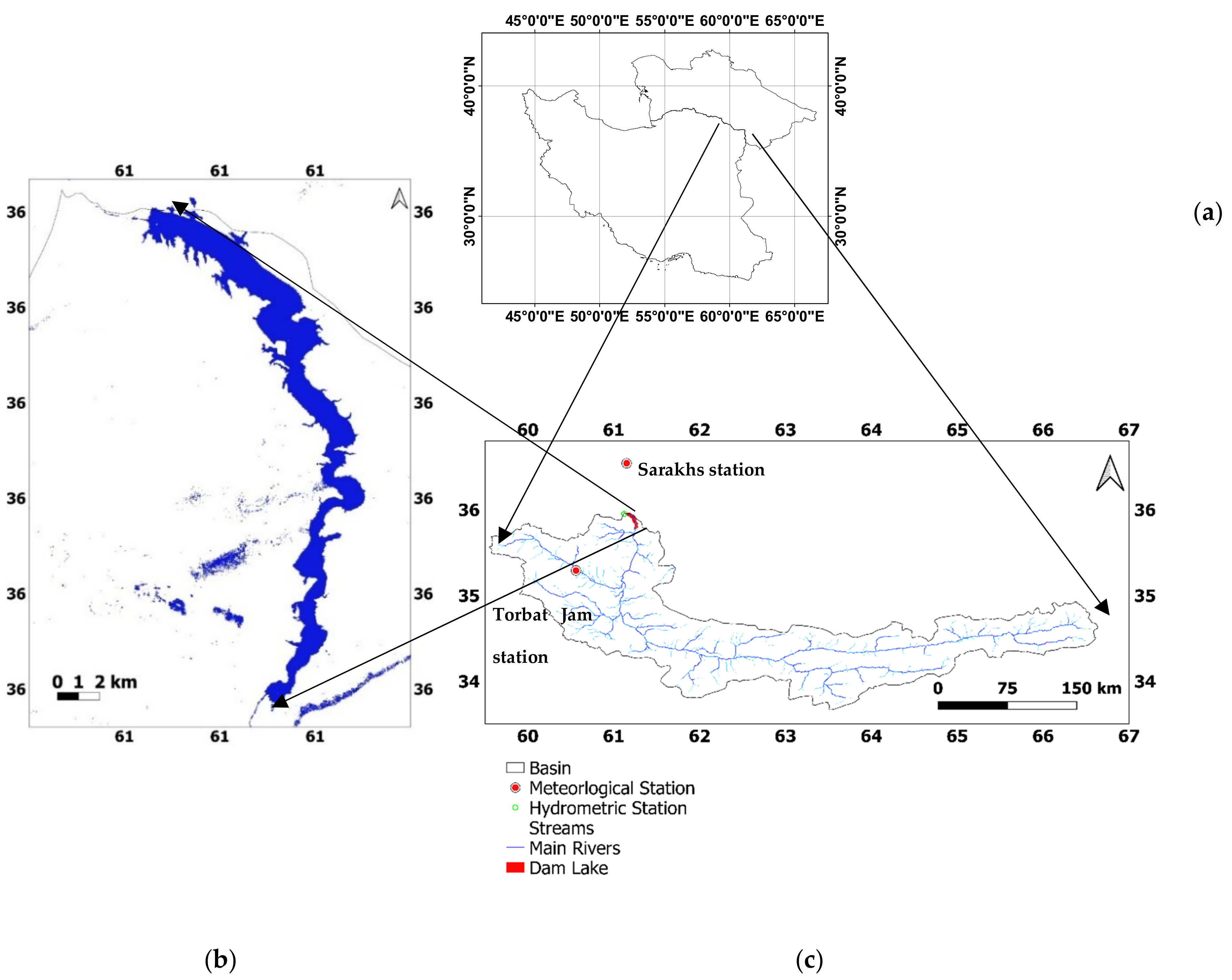
2.1. Study Region

The Doosti Dam’s basin (Figure 1) is the biggest transboundary basin between two countries, Iran and Turkmenistan, and is located between latitude 33° N to 36° N and longitude 59° E to 67° E. The basin covers an area of approximately 55,141 km², and the climate of this region is semi-arid and the reservoir of the dam is a clear and relatively deep lake with a maximum and mean depth of 35 m and 15 m, respectively [17,18]. The Doosti Dam is important for Iran as the country relies on its role in supplying fresh water to Mashhad, the second-most populous city in Iran with a population of around 3 million. The dam provides drinking water for up to 76% of the population in Mashhad and its principal tributaries, mostly for the purpose of storing water in reservoirs, irrigation for agriculture, and producing electricity.

Mashhad is a great example of a city that depends heavily on outside imports of water and power. Due to the city’s fast growth, climate change and severe droughts, and eightfold expansion of the population, Mashhad’s local water supplies are under a lot of stress. The city is now considerably more dependent on water from far-off sources as a result [29].

Iran’s approach to water management is reactive rather than proactive, putting more emphasis on quick fixes such as expanding the number of wells and dams and transporting water from far-off sources rather than on looking for fresh opportunities and long-term solutions to address any threats or issues before they arise.

2.2. Datasets

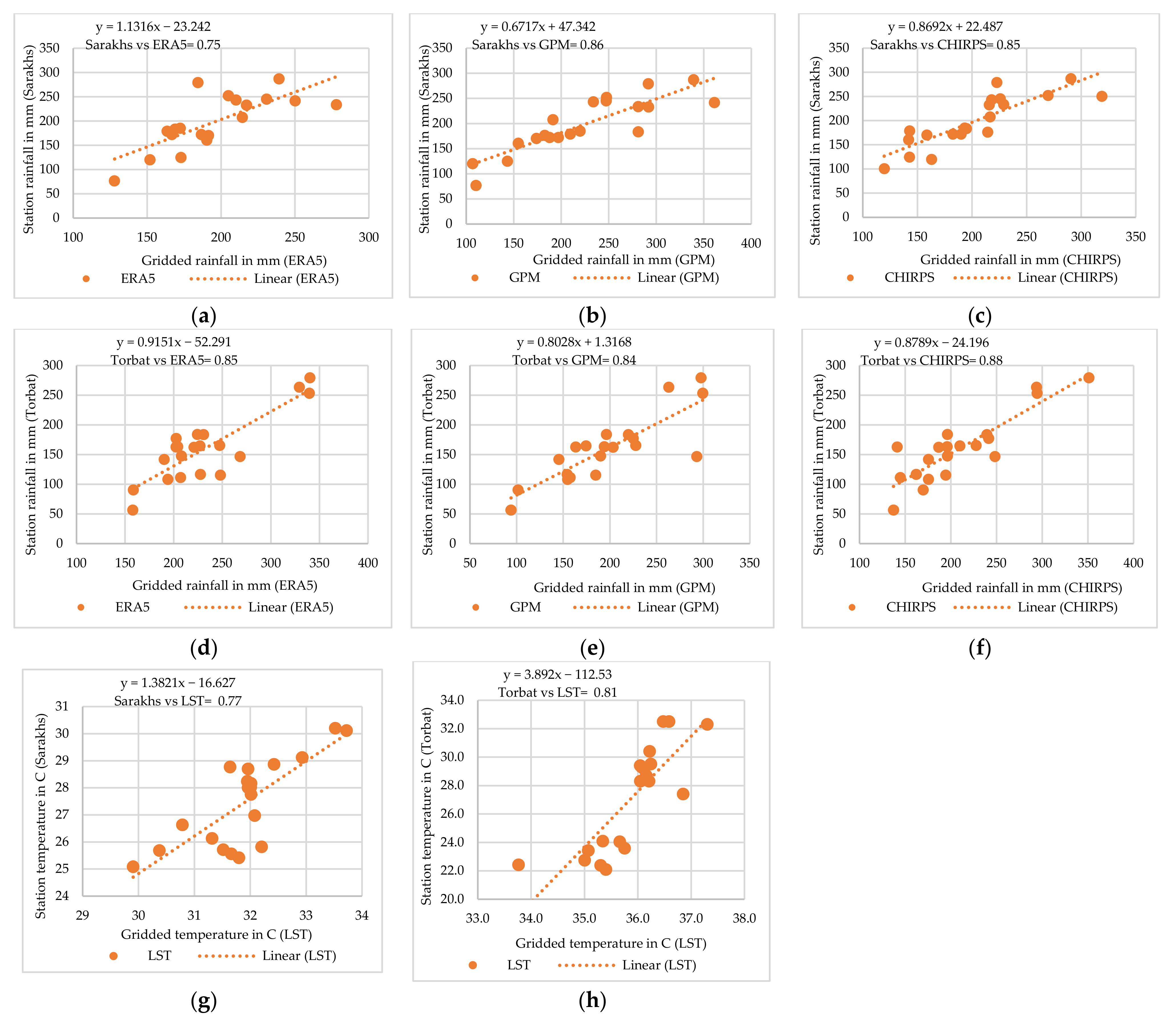
2.2.1. Ground Measurements

The daily hydroclimatologic parameters consisting of precipitation and temperature collected from three local stations are presented in

Table 1. Specifications of ground-based data used in evaluation of satellite-based data.

Station	Specifications	Longitude (m)	Latitude (m)	Elevation (m)	Time Scale	Period
Torbat Jam	Meteorology station	60.56	35.29	950	Daily	2001–2020
Sarakhs	Meteorology station	61.15	36.54	278	Daily	2001–2020

. Because of the lack of field data, remotely sensed data could be a good alternative in this study. Faulty gauge stations can create some gaps in the collection of hydrological time series data. Most often, the upstream and downstream data exchange between the two riverine countries has not been effective. Data collecting across borders must be independent between nations in order to quickly determine the amount of inundation for emergency response activities [38]. Remote sensors mounted on satellites and aircraft have the capability to provide data [39].

2.2.2. Satellite Data

Within each year, surface water varied on a regular basis and, in remote sensing, the use of multispectral satellite data is known to be well suited for trend analysis given its high-spectral correlation with open water surfaces and the accuracy of mapping [40].

We used a rich time series of remote sensing data to gather further details about the scope of this study. The remote sensing data used in this study included the Climate Hazards Group InfraRed Precipitation With Station (CHIRPS) dataset (500 m spatial resolution), MODIS Terra Evapotranspiration (MOD16A2) (500 m spatial resolution), MODIS Terra snow cover MOD10A1 (500 m spatial resolution), MODIS LST MOD11A1 (1 Km spatial resolution), MODIS NDVI MOD09GQ (250 m), Landsat TM/ETM+/OLI (30 m spatial resolution), SRTM (NASA SRTM Digital Elevation 30 m) were obtained from the online dataset provided by GEE. A framework of this study is presented in Figure 2.

In order to assess the effectiveness of the satellite-based rainfall data, different satellite-based rainfall data were examined.

Table 2. Comparing observed and gridded datasets’ (CHIRPS, GPM and ERA5 for rainfall and LST for temperature) spatial similarities using statistical indices for the period from 2001 to 2020.

Statistical Measurements	Rainfall Station (mm), Sarakhs	Rainfall Station (mm), Sarakhs	Rainfall Station (mm), Sarakhs	Rainfall Station (mm), Torbat	Rainfall Station (mm), Torbat	Rainfall Station (mm), Torbat	Temperature Station (°C), Sarakhs	Temperature Station (°C), Torbat
	CHIRPS	GPM	ERA5	CHIRPS	GPM	ERA5	LST	LST
R2	0.71	0.74	0.56	0.77	0.71	0.73	0.61	0.66
Pearson’s correlation	0.85	0.86	0.75	0.88	0.84	0.85	0.77	0.81
RMSE	25.27	34.28	35.59	48.57	49.23	66.16	4.56	9.25
Bias	5.6	19.7	−2.36	40.40	37.55	59.12	4.44	8.75
MBias	1.02	1.13	0.98	1.31	1.23	1.45	1.16	1.32

demonstrates the results of descriptive statistics that show reasonable spatial agreement with gauge and gridded data. All the rainfall satellite datasets overestimated the stations’ rainfall, with R² and Pearson correlation in the Sarakhs and Torbat-Jam stations varying from 0.71 and 0.85 for CHIRPS to 0.56 and 0.75 for ERA5, and from 0.77 and 0.88 for CHIRPS to 0.71 and 0.84 for GPM, respectively. The minimum RMSE was represented by CHIRPS (5.6 mm) for Sarakhs and CHIRPS (48.57 mm) for Torbat, whereas ERA5 exhibited maximum RMSE (35.59 mm) and (66.16 mm). CHIRPS was chosen for trend analysis as it represents better performance for all the gauge stations (Table 2); and it has a spatial resolution of 5 km which is more accurate compared to other gridded rainfall data and has low systematic bias. Similarly, Land Surface Temperature (LST) overestimated the stations’ temperature with R² 0.66 and 0.61 and RMSE 9.25 °C and 4.56 °C in Torbat-Jam and Sarakhs stations, respectively.

Figure 3a–f shows Pearson correlation for both observational and gridded data, revealing strong spatial agreement with CHIRPS. All three gridded datasets were well matched, although CHIRPS had greater agreement with the Sarakhs station (r = 0.85) and Torbat station (0.88) than GPM (0.86) and ERA5 reanalysis (0.75). Figure 3g–h illustrates the similar relationship with the LST datasets. According to the results, LST overestimated temperature for the two stations’ data, Sarakhs and Torbat, in the region.

MODIS Data

LST is an extremely important parameter that controls the exchange of longwave radiation and sensible heat flux between the Earth’s surface and the atmosphere. Therefore, trend analysis of LST is essential for the study of the hydroclimatology behaviour of basins. Generally, LST products are derived from thermal infrared (TIR) sensors (e.g., AVHRR, MODIS or METEOSAT) [41].

Among the TIR sensors, the LST products of MODIS aboard the Terra and Aqua platforms’ data have high quality, global coverage and accurate geolocation [42]. Daily MODIS LST products [43] are retrieved at 1 km pixels by the generalised split-window algorithm. The daily average land surface temperature was extracted from the MODIS [44].

Because of snow’s influence on Earth’s climate and its role in supplying water resources, in many mountainous areas such as upstream of Doosti Dam, it is necessary to monitor snow cover extent (SCE) and snow properties in both high temporal and spatial resolutions. For more than three decades, optical, infra-red (AVHRR, MODIS) and passive microwave satellite sensors (SSMI/S, AMSR-E) have been used to monitor the extent of snow areas effectively [45]. Although cloud cover often obscures the snow from visible/infra-red spaceborne sensors, due to high spatial and temporal resolution, the MODIS snow products (MOD10A1) [46] with a resolution of 500 m at daily scale are preferred for snow-cover monitoring.

To quantify the vegetation dynamics over space and time and derive the irrigated cultivated lands, MODIS surface reflectance (MODIS/Terra MOD09GQ) [47] with 250 m spatial resolution and daily temporal resolution was implemented from 2001 to 2021. Maximum NDVI maps in the periods of April to June and July to September were used to derive the cultivated areas in the winter and summer agriculture seasons, respectively. A threshold value of 0.5 for NDVI was considered as an indicator of the cultivated agriculture area. Considering the prevalence of surface irrigation in the region, the irrigated cultivated lands were derived by applying a defined elevation range from the river baseline on the DEM map. Topographic information, including the catchment’s elevation, was collected using the Shuttle Radar Topography Mission (SRTM) and digital elevation models (DEMs) 90 m from GEE. For evapotranspiration, MODIS/Terra Net MOD 16A2 evapotranspiration (version 6, 8 day L4 datasets) was launched from 2000 with a pixel resolution of 500 m applied [48].

Landsat Images

Water surface areas are regularly determined from optical satellite imagery such as MODIS and Landsat products [49,50]. Changes in lake distribution have been monitored using the MODIS and Landsat datasets [51]. Landsat has a high resolution (30 m), which is its main benefit, but it also has a low repetition frequency [4]. To produce the water mask of the Doosti reservoir, NDWI maps derived from Landsat images from 2001 to 2020 were implemented. Landsat images consisting of ETM+ [52] and OLI data were acquired from GEE. NDWI maps [53,54] were generated based on Green [55] and NIR bands, and the pixels with positive value were assigned as water class. Specifications of all satellite data used in this research are listed in

Table 3. Specifications of used datasets of satellite imagery available in Google Earth Engine.

Parameters	Temporal Resolution	Product Information	Spatial Resolution	Time Period
CHIRPS	Daily	Climate Hazards Group InfraRed Precipitation with Station Data (Version 2.0 final)	5 km	2001–2021
GPM	Daily	Global Precipitation Measurement (GPM)	10 km	2001–2020
ERA5		European Centre for Medium-Range Weather Forecasts (ECMWF) Climate Reanalysis	25 km	2001–2020
MODIS Terra	Daily	Surface reflectance (MOD09Q)	250 m	2004–2021
	Daily	Snow cover (MOD10A1)	500 m
	Daily	Land Surface Temperature (MOD11A1)	1 km
	8-Day	Evapotranspiration (MOD16A2)	500 m
Landsat 5 TM	16 days	Level 1	30 m	2004–2021
Landsat 7 ETM	16 days	Level 1	30 m	2004–2021
Landsat 8 OLI	16 days	Level 1	30 m	2013–2021
DEM	1	SRTM	90 m	-

. A code was developed within the GEE environment to compute the time series of lake area statistics (maximum, minimum, mean and standard deviation) from 2004 to 2021.

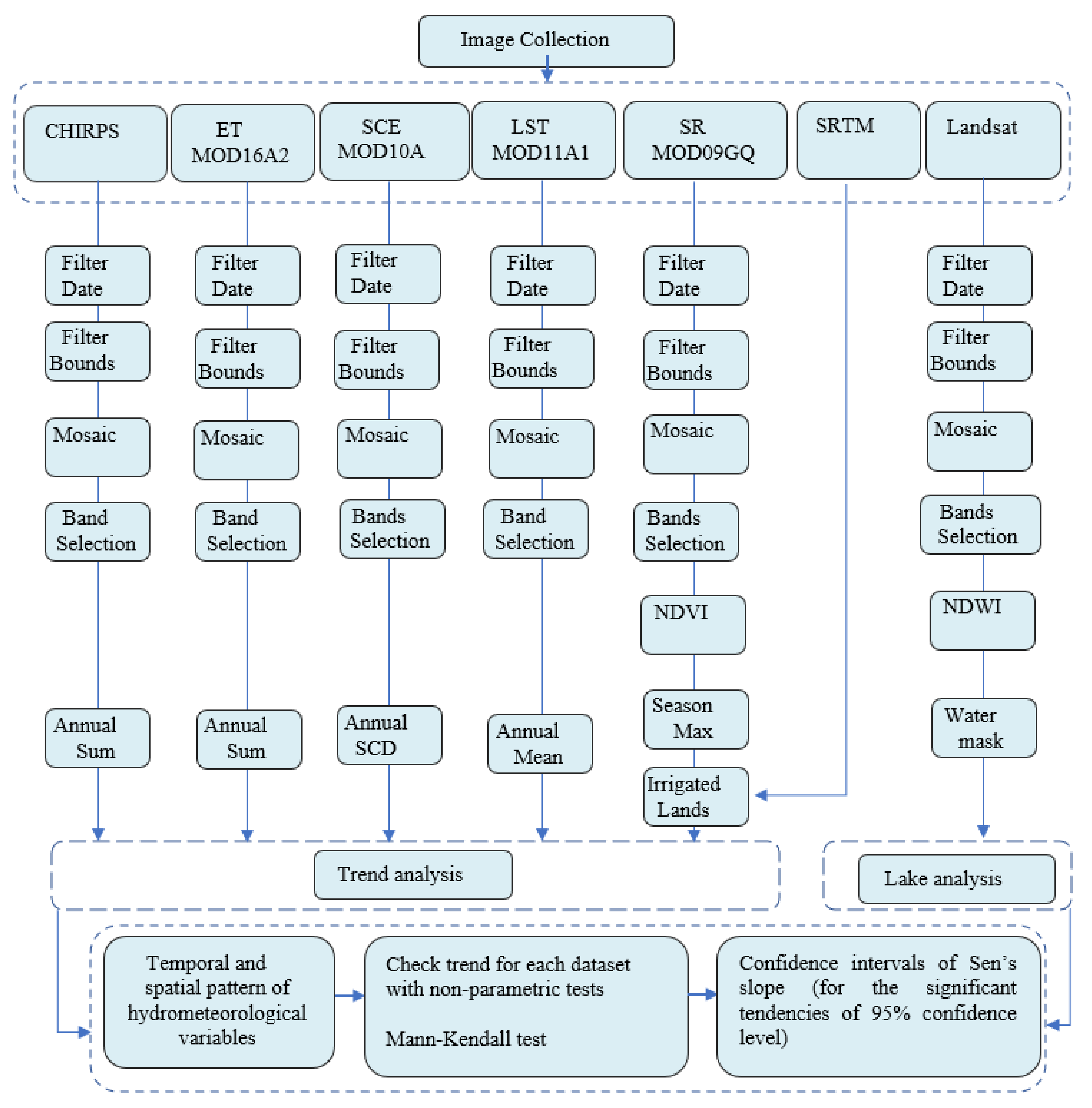
2.3. Methods

The GEE platform contains a substantial amount of satellite data acquired by other missions and it also hosts other ancillary data such as digital elevation models, vector-based datasets, land cover and meteorological data [56]. Since data hosted by GEE is analysis-ready, the need for pre-processing is circumvented as these data have been found to be consistent over time and well-suited for time series analysis and estimating long-term trends [14]. By applying the date filter function to the image collections, the desired time periods (2004–2021) were separated from the whole datasets. The spatial filter function was used to limit the borders to the Doosti Dam watershed. Then, using the trend functions (Mann–Kendall, Sen’s slope) in GEE, evaluation of the pixel-based long-term spatiotemporal trend for the gridded datasets was carried out to analyse the trend and its intensity. The Mann–Kendall expression (alpha 0.05 and Z statistics = 1.96, generated from the standard normal table) was used to assess the Sen’s slope [57].

2.3.1. Mann–Kendall Trend and Sen’s Slope Test

The Mann–Kendall (MK) and Sen’s slope estimator was applied using programming in GEE to compute the long-term magnitude of change on hydroclimate datasets and their statistical significance. The MK statistical test [58,59,60] was used to quantify the significance of trends in meteorological time series [57,61]. The MK test null hypothesis (H0) says that there is no monotonic trend at the specified level of significance. This may be used to detect the monotonic trend in a time series. In this test, the alternative hypothesis (Ha) suggests that the data exhibit a monotonic trend over time that is described by Equation (1):

$${\mathrm{S}}_{\left(k, l\right)}={{\displaystyle \sum }}_{i=1}^{n-1}{{\displaystyle \sum }}_{j=i+1}^{n}sgn\left(X_{j\left(k, l\right)}-X_{i\left(k, l\right)}\right)$$

(1)

where n is the number of data points, $X_{i\left(k, l\right)}$ and $X_{j\left(k, l\right)}$ are the data values in the time series i and j ($j>i$), respectively, k and l indicate point location in the data matrix and $sgn\left(X_{j\left(k, l\right)}-X_{i\left(k, l\right)}\right)$ is the sign function, as illustrated in Equation (2).

$$sgn\left(X_{j\left(k, l\right)}-X_{i\left(k, l\right)}\right)=\left\{\begin{array}{c}+1 if X_{i\left(k, l\right)}-X_{j\left(k, l\right)}>0\\ 0 if X_{i\left(k, l\right)}-X_{j\left(k, l\right)}=0\\ -1 if X_{i\left(k, l\right)}-X_{j\left(k, l\right)}=0\end{array}\right.$$

(2)

In cases where the sample size $n>30$, the standard normal test statistic Z_S(l,k) is computed using Equation (3):

$$Z{s}_{\left(k, l\right)}=\left\{\begin{array}{c}\frac{S_{\left(k, l\right)}-1}{\sqrt{Var\left(S_{\left(k, l\right)}\right)}} if S_{\left(k, l\right)}>0\\ 0 if S_{\left(k, l\right)}=0\\ \frac{S_{\left(k, l\right)}+1}{\sqrt{Var\left(S_{\left(k, l\right)}\right)}} if S_{\left(k, l\right)}<0\end{array}\right.$$

(3)

Positive values of Z_S(l,k) indicate increasing trends while negative Z_S(l,k) values show decreasing trends. A two-tailed test was conducted using the hypothesis test technique at alpha = 50% level of significance, with the null hypothesis being no monotonic trend in time series at the 95% level of significance ($H_0: \tau =0$) and the alternative hypothesis being a substantial monotonic trend in time series in the 95% significance level ($H_a: \tau =0$) [62].

Sen’s nonparametric method [63] was used to estimate the magnitude of trends in the time series:

$$T_{i\left(\mathrm{l},\mathrm{k}\right) }=\frac{X_{j\left(\mathrm{l},\mathrm{k}\right) }-X_{i\left(\mathrm{l},\mathrm{k}\right) }}{j-m}$$

(4)

In this equation, $X_j$ and $X_k$ represent data values at time j and m, respectively, Consider

$$Q_{i\left(\mathrm{l},\mathrm{k}\right) }=\left\{\begin{array}{c}{T}_{\left(N+1\right)/2} N is odd\\ \\ \frac{1}{2}\left(T_{N/2}+T_{(N+2)/2}\right) N is even.\end{array}\right. .$$

(5)

A positive $Q_{i\left(\mathrm{l},\mathrm{k}\right) }$ value represents an increasing trend and a negative $Q_{i\left(\mathrm{l},\mathrm{k}\right) }$ value represents a decreasing trend over time.

2.3.2. Descriptive Statistics

To ensure high-quality satellite rainfall data with respect to station observed data, several statistical indices were employed to check the effectiveness and performance of satellite datasets [57]. Statistical measurements [6], including the correlation coefficient (R²), bias, multiplicative bias root (MBias), mean absolute error (MAE) and root mean square error (RMSE), were performed to assess data distribution and the relative performance of the satellite datasets, thus ensuring high-quality satellite data (rainfall, lake water) with regard to gauge measurements as follows (Equations (6)–(9)):

$$R^2={\left(\frac{\frac{1{{\displaystyle \sum }}_1^n\left(X_{obs}-X_{obs}\right)\left(X_{sat}-X_{sat}\right)}{n}}{X_{obs}\times X_{sat}}\right)}^2$$

(6)

$$\mathrm{RMSE}=\sqrt{{{\displaystyle \sum }}_1^{\mathrm{n}}\frac{{\left({\mathrm{X}}_{\mathrm{sat}}-{\mathrm{X}}_{\mathrm{obs}}\right)}^2}{\mathrm{n}} }$$

(7)

$$\mathrm{Bias}=\frac{{{\displaystyle \sum }}_1^{\mathrm{n}}\left({\mathrm{X}}_{\mathrm{sat}}-{\mathrm{X}}_{\mathrm{obs}}\right)}{\mathrm{n}}$$

(8)

$$\mathrm{MBias}=\frac{{{\displaystyle \sum }}_1^{\mathrm{n}}\left({\mathrm{X}}_{\mathrm{sat}}\right)}{{{\displaystyle \sum }}_1^{\mathrm{n}}\left({\mathrm{X}}_{\mathrm{obs}}\right)}$$

(9)

In which, X_obs and X_sat show the gauge and satellite time series, respectively; n is the total number of observations; and ${\overline{X}}_{obs}$ the average of station values.

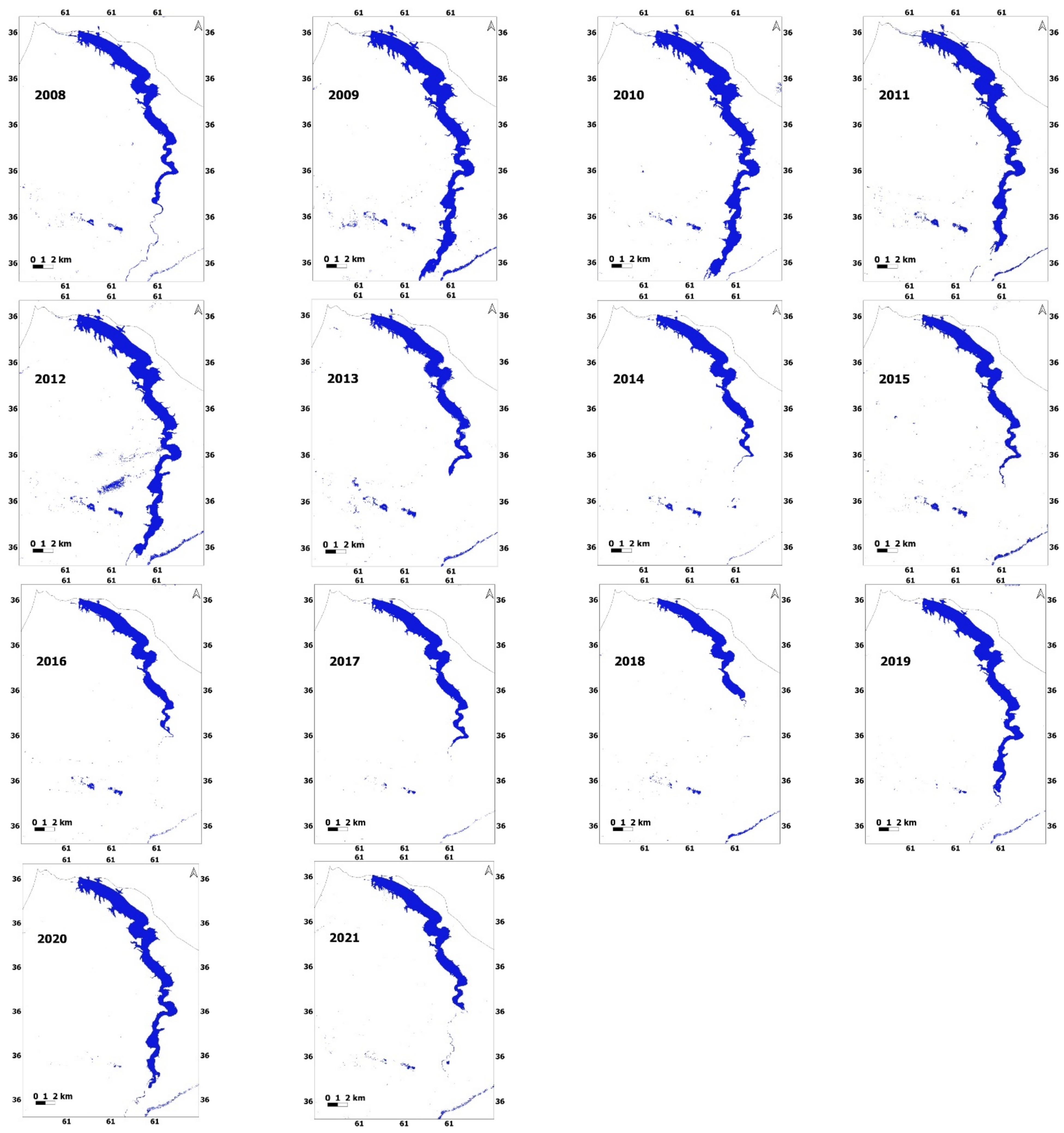
3. Results

3.1. Temporal Pattern of Different Hydroclimatic Factors

The underlying structure of the Doosti Dam basin’s images, monitored from 2004 to 2021, was investigated (Figure 4). The satellite images reveal a downward trend until 2018. Figure 4 shows the extent of the Doosti Dam’s reservoir in the early spring of the years between 2004 and 2021. As illustrated in Figure 4, the water stored in the dam reservoir has decreased over time from 2013 to 2018, which is a sign of the reduction in water input. During these 18 years, the reservoir has had the lowest area in 2018 and the highest area in the early spring of 2009–10.

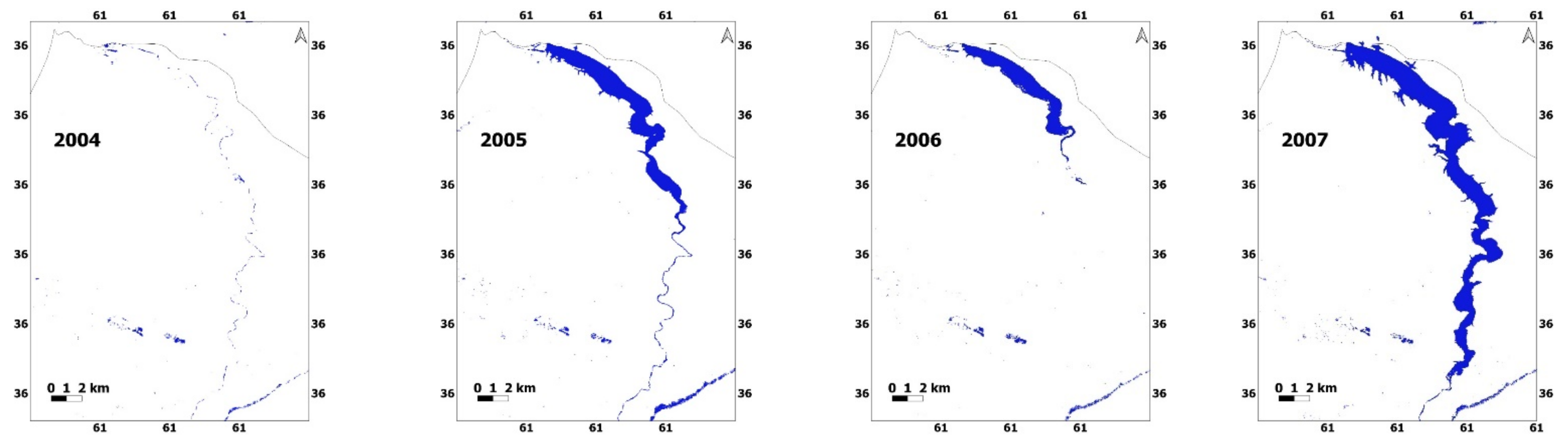
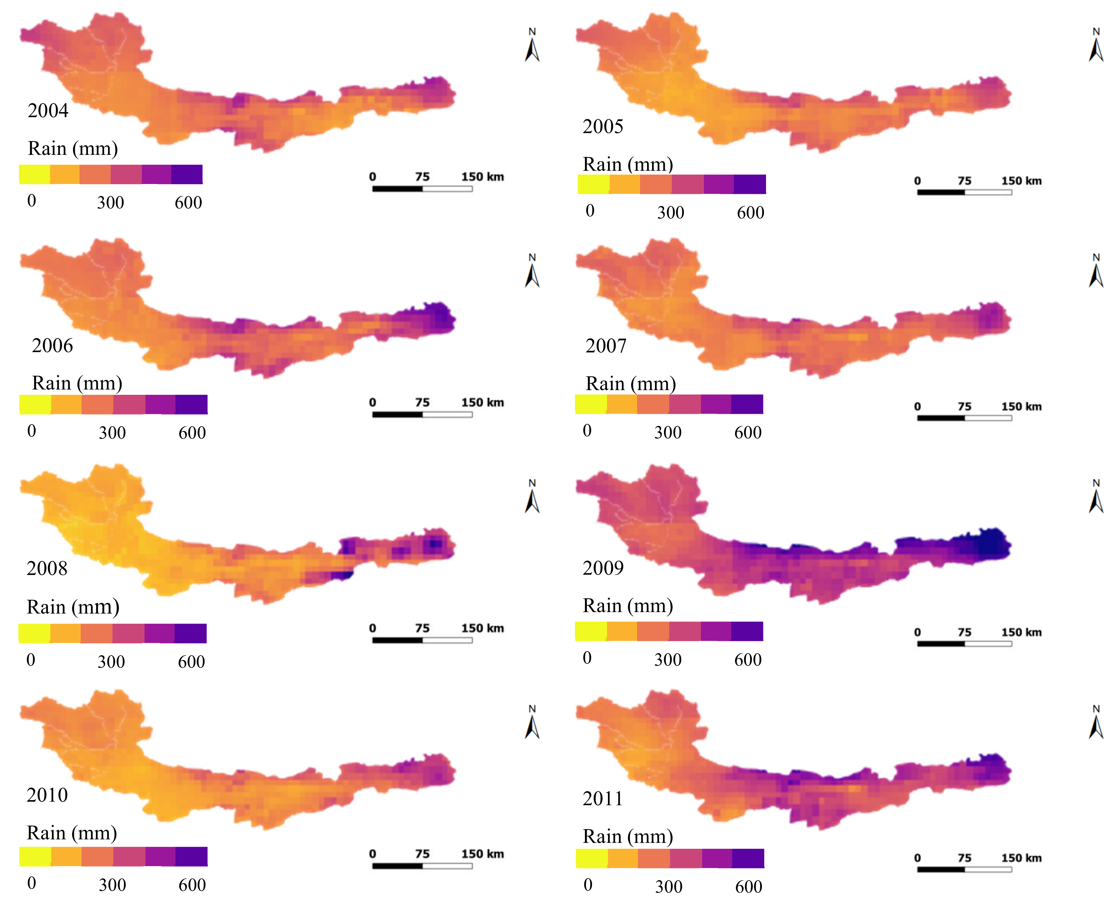
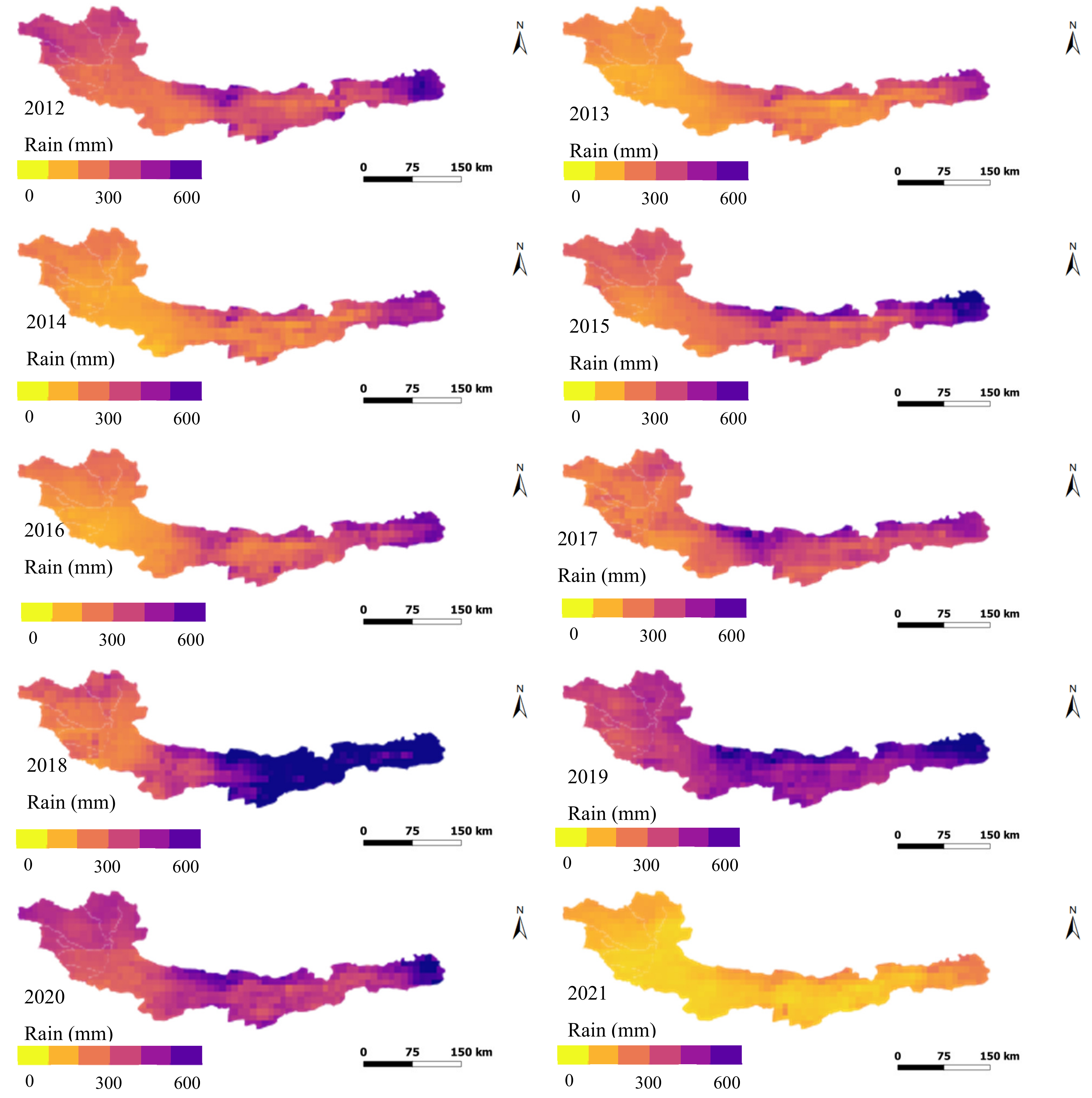
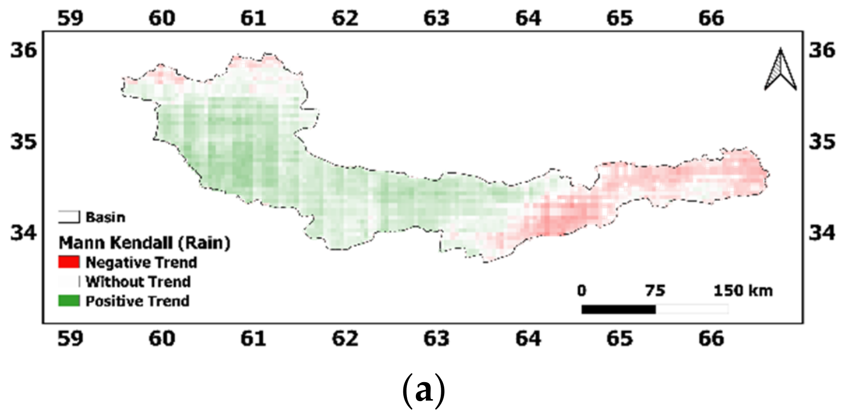
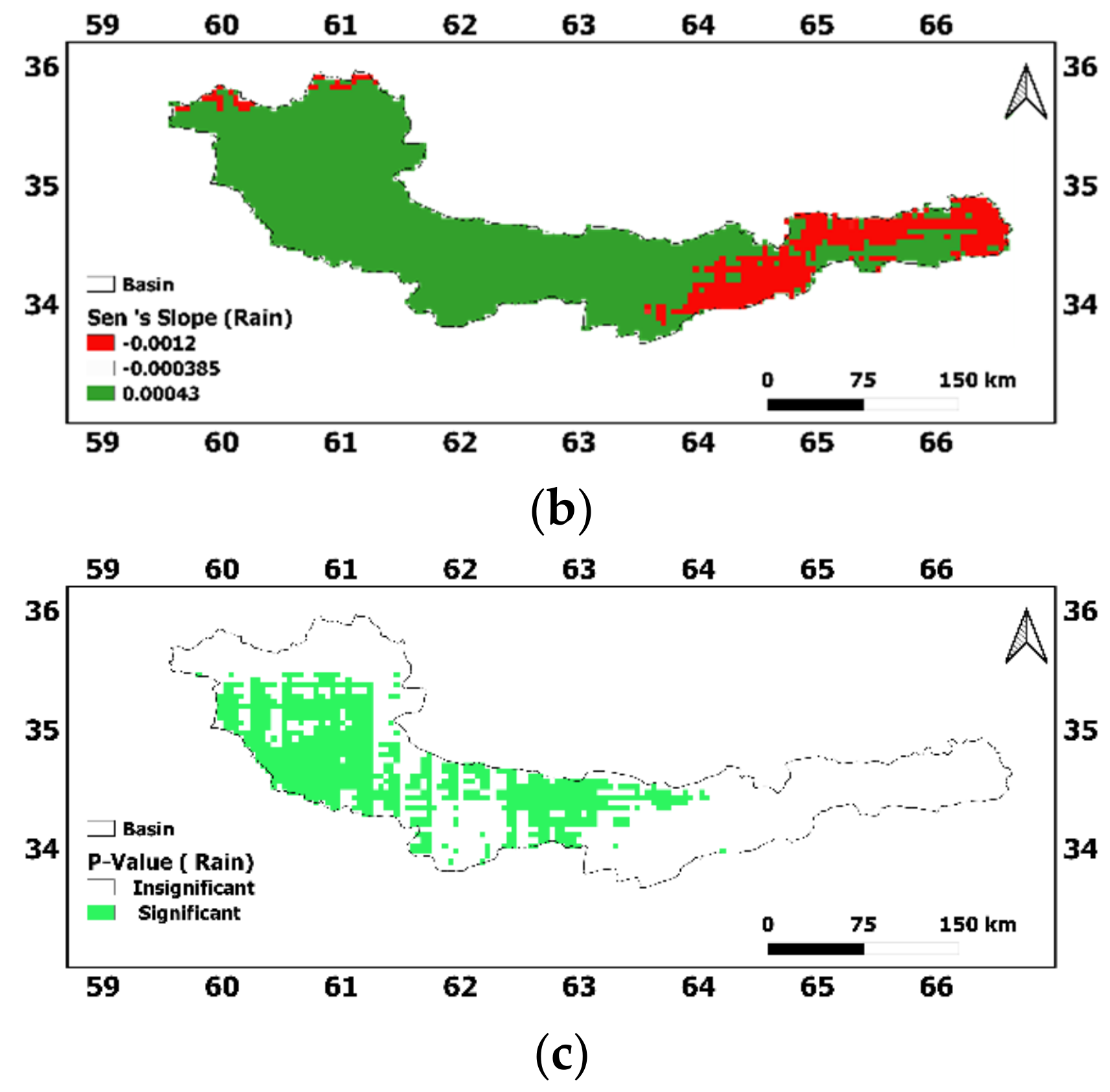
3.2. Spatiotemporal Distribution of Rainfall in the Doosti Dam Basin (2004–2021)

To identify the trends of precipitation and provide better insight into how precipitation is distributed over the catchment, the spatial–temporal variation of the annual CHIRPS precipitation [64] for the period of 2004–2021 is displayed in Figure 5. In this figure, the areas with the highest precipitation are shown in red and the areas with the lowest precipitation are colored light orange. Rainfall is highest in the mountainous region southeast of the catchment, located mainly on the Turkmenistan borders, upstream (500 mm) especially in 2009, 2011, 2015, 2019 and 2020. However, in lower elevation areas, the basin downstream experienced the lowest rainfall (100 mm). The annual precipitation varied from 100 mm to approximately 600 mm. The effects of climate change at a local level must be evaluated because it is a global issue and analysing rainfall trends is a necessary first step in determining how climate change may affect the availability of water and food security. The years 2018, 2019 and 2009 experienced the maximum increase (600 mm) in the whole basin, especially the mountainous areas in the west and east. The years 2005, 2008 and 2021 experienced marked minimum rainfall (100 mm). The results also confirm that the mountainous regions of the basin are the wettest regions.

Figure 6 shows the spatial distribution of trends in the annual precipitation based on CHIRPS estimates for the period from 2004 to 2021. The spatial pattern of the MK test shows that precipitation increased in most regions of the Doosti Dam’s basin (Figure 6a), and from the statistical point of view, this trend is significant at a 95% level of confidence for annual precipitation. Figure 6b, shows an increasing trend in rainfall in the middle and west regions of the basin with a Sen’s slope calculation which varies from 0.00043 (upper limit) to −0.00012 (lower limit) (p-value < 0.05) for upward and downward trends for the significant tendencies at 95% confidence level, respectively. Moreover, a statistically significant increasing tendency was detectable across the center and downstream of the region (+0.00043). The p-value is less than alpha = 0.05, indicating that there was a trend in the time series. So, the results clearly demonstrate that in most parts of basin, especially center to downstream (p-value = 0.5), an upward trend with a 95% confidence level is observed; however, there was no significant trend in the upstream, as illustrated in Figure 6c. In Figure 6b, the Sen’s slope and MK test indicate that rainfall trends show climate change has occurred in the basin.

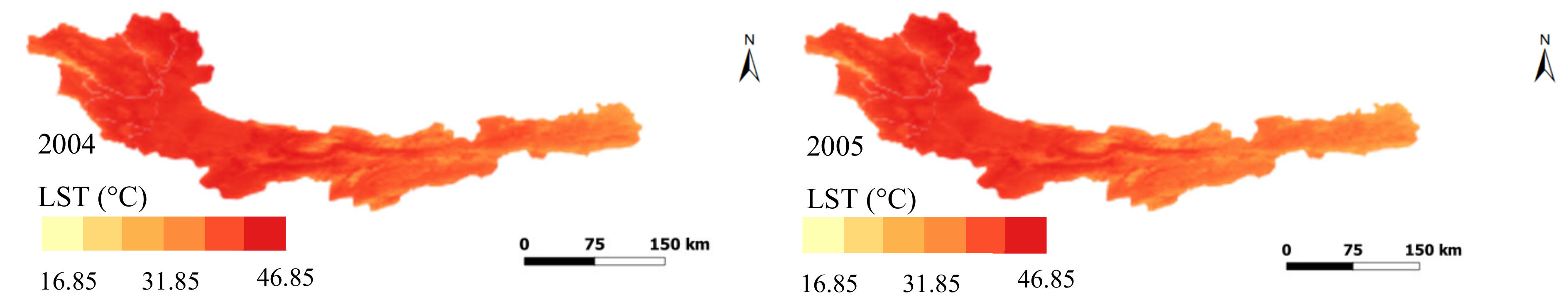
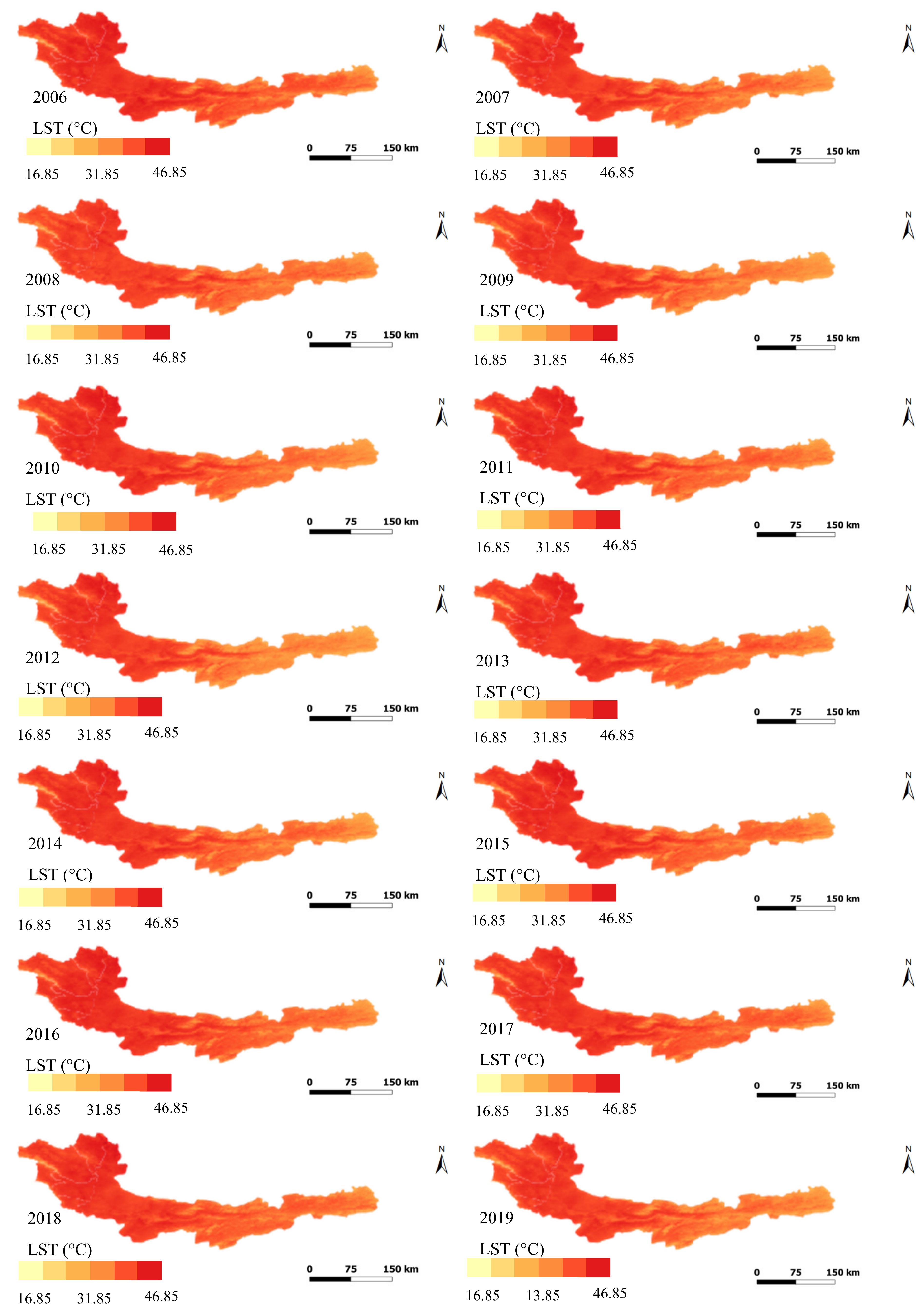
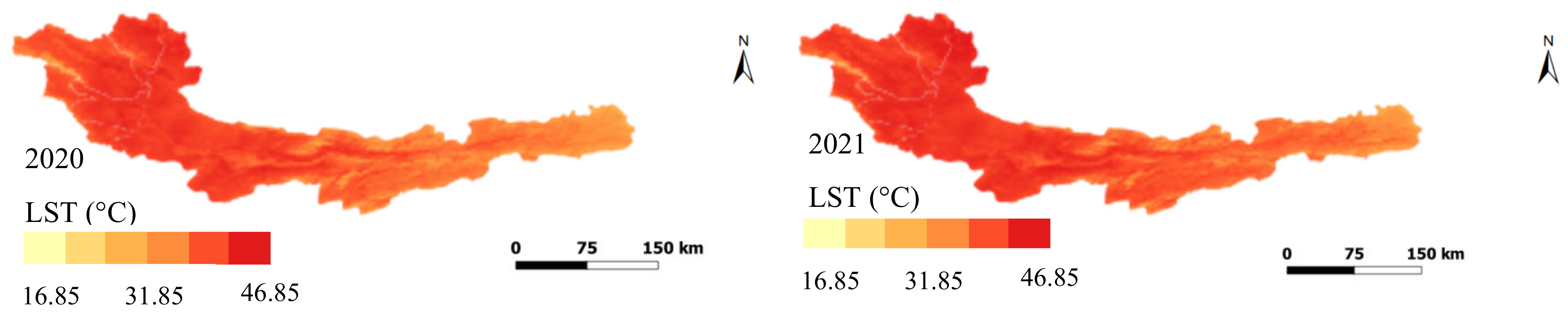
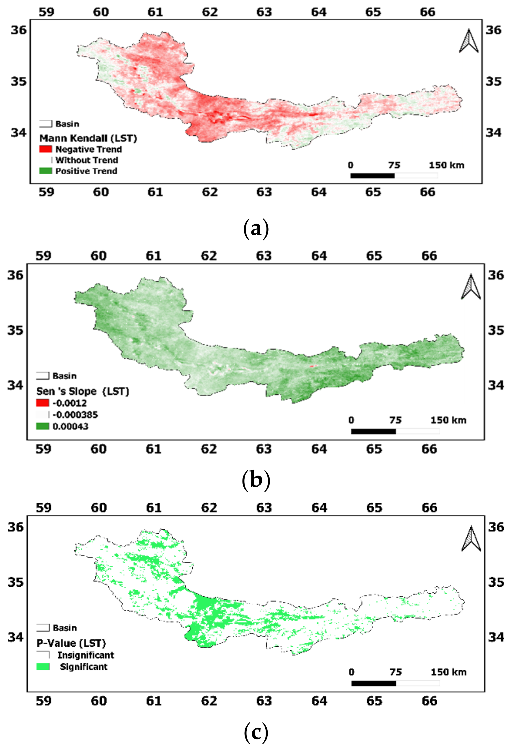
3.3. Spatio-Temporal Distribution of Temperature (LST) in the Doosti Dam Basin (2004–2021)

Temperature extremes are detrimental to agriculture, health, and infrastructure such as hydraulic structures and economic activity. This study investigates the annual temperature distribution and trend of LST from the MODIS Terra (MOD11A1) for the period 2004–2020. As predicted, temperature is strongly influenced by elevation. Figure 7 shows that the highest annual LST (averaging 30.85 °C) occurred at the lowest elevation level surface (Doosti Dam’s basin upstream). As shown in this figure, LST follows the topography of the earth, and the highest elevation areas have lower temperatures (Doosti Dam’s basin upstream). Most agricultural lands are located alongside the Doosti Dam’s river downstream, where higher temperatures were observed. The temperature varied from 26.85 °C to 36.85 °C. There is greater annual spatial variability at the lower elevation area, ranging between 31.85 °C and 41.85 °C. The results also illustrate that the central south area of the basin experienced the highest temperatures for the period 2004 to 2021.

Figure 8a shows the spatial distribution of trends in the annual temperature, based on MODIS (MOD11A1) estimates for the period between 2004 and 2021. The spatial pattern of the Mann–Kendall test showed that temperature decreased in the centre to east of the Doosti Dam’s basin (Figure 8a) with a 95 % confidence level, as shown in Figure 8c (p-value < 0.05). The increase in slope of temperature distinguished by Sen’s slope is illustrated in Figure 8b. LST exhibits a variation of 29 °C to 31.85 °C, with low annual precipitation varying from 100 mm to 400 mm, indicating that agriculture in these areas is not possible without irrigation.

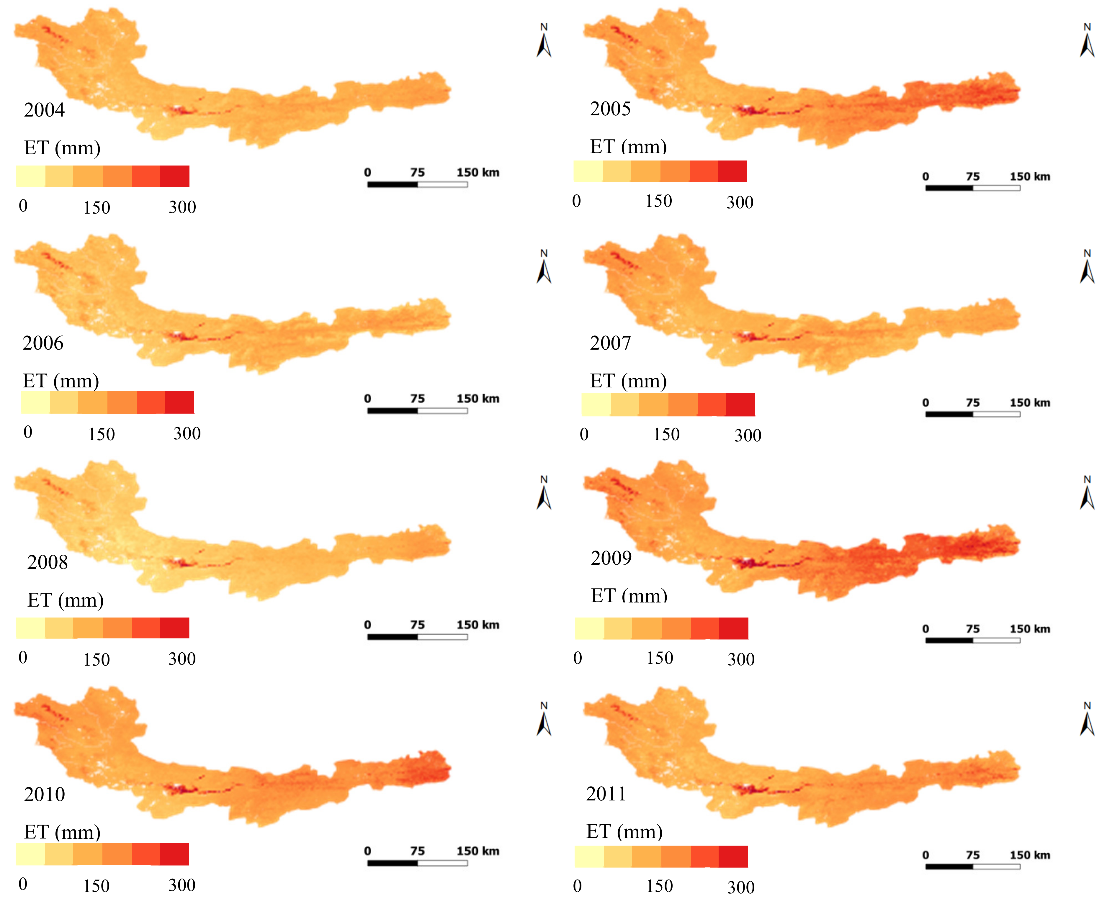
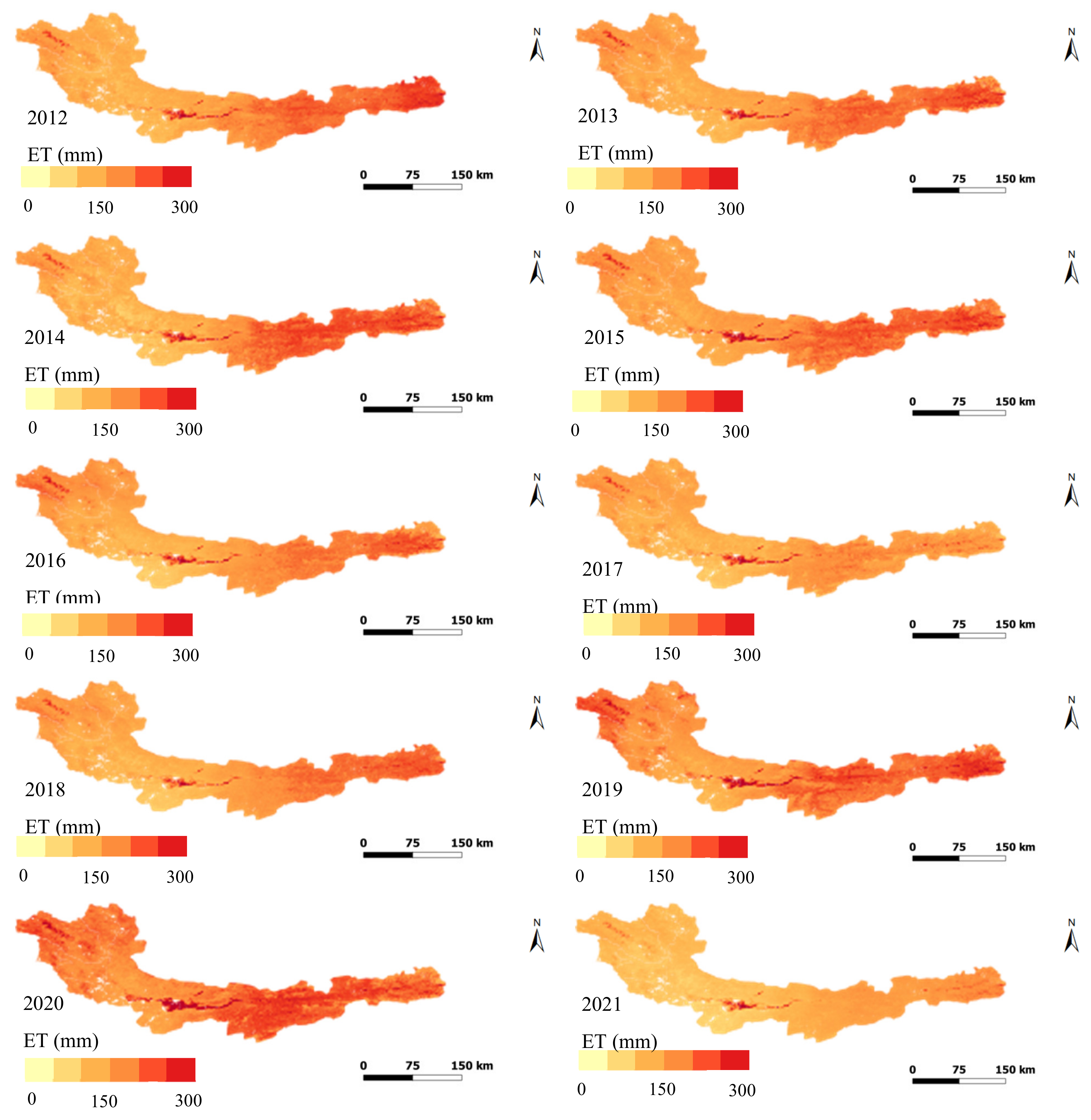
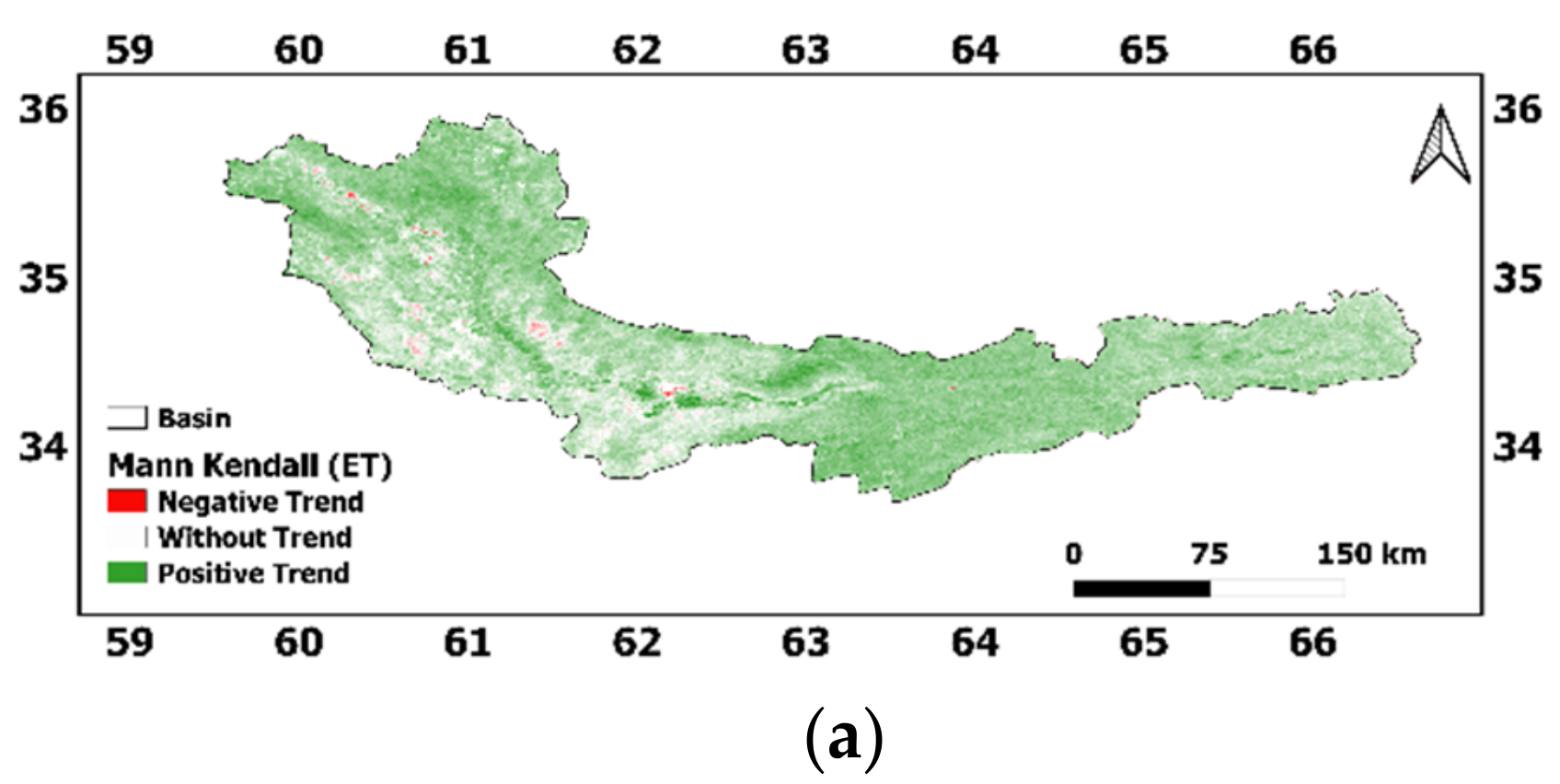
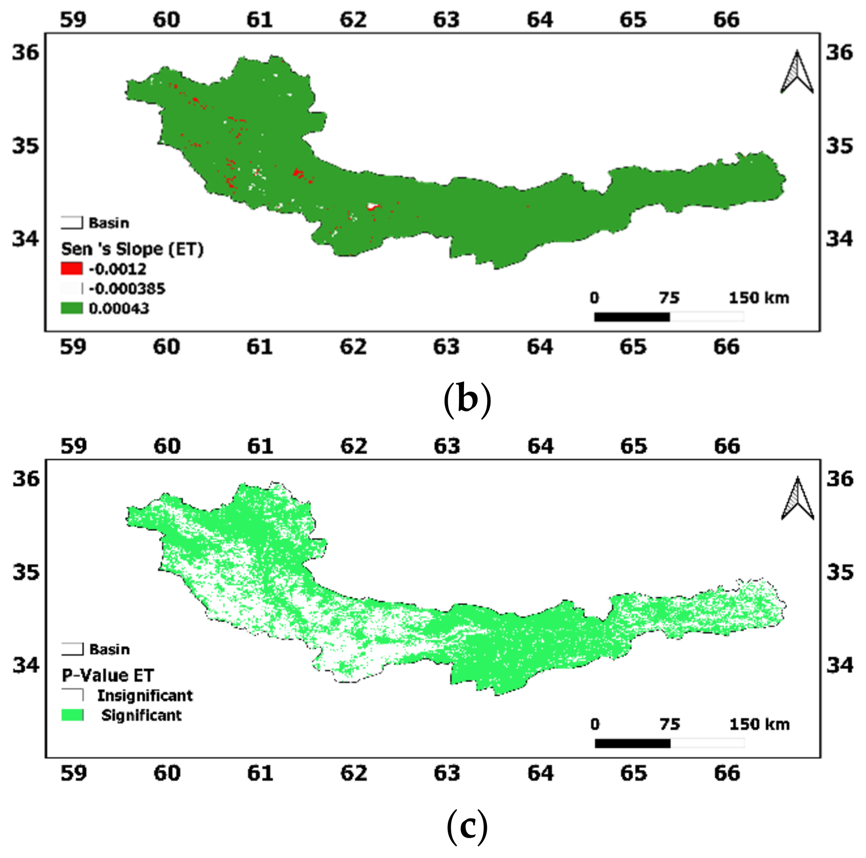
3.4. Spatio-Temporal Distribution Annual Evapotranspiration from MODIS in the Doosti Dam’s Basin (2004–2021)

An analysis of annual distribution and the trend of evapotranspiration offers a more detailed illustration of the increase in water demand causing more water deviation from the river. Figure 9 depicts the importance of evapotranspiration losses which varied from 100 to 200 mm in the basin. From this figure, it can be seen that the periods from 2004 to 2008 had low evaporation loss areas, while the period from 2009 to 2020 experienced high water demand. It also shows that the high elevation areas were underwent higher evapotranspiration (near 200 mm) than the downstream areas (Iranian side). The river line in the center shows the slight and constant evapotranspiration and water demand expanding from the west to the east. Mean annual evapotranspiration (2005–2020) in the Doosti Dam River was observed to be 200 mm across the basin. Interestingly, both precipitation and evapotranspiration have almost identical trends. The precipitation and evapotranspiration exhibited the highest increases in the year 2009 (~500 mm) and (~170 mm), and for year 2019 (~550 mm) and (~200 mm), respectively. This also confirms that the whole basin represents an increasing trend, especially the mountainous areas in the east and alongside the river.

Figure 10 shows the spatial distribution of trends in the annual evapotranspiration based on the MODIS product (MOD16A2) estimates for the period from 2004 to 2021. The spatial pattern of the MK test shows that evapotranspiration is rising in the whole region of the Doosti Dam’s basin (Figure 10a), and from the statistical point of view, this increasing trend is significant with the positive trend at a 95% level of confidence for annual evapotranspiration. In Figure 10b, evapotranspiration is observed to have an increasing trend (+0.00043) during the years 2004–2021 in the whole study area.

This figure reveals a rising trend in evapotranspiration in the regions of the basin with a Sen’s slope calculation which varies from +0.00043 (upper limit) to −0.0012 (lower limit) for upward and downward trends for the significant tendencies at a 95% confidence level, respectively. Moreover, a statistically significant increasing tendency is detectable across the region (+0.00043). Figure 10c shows that evapotranspiration rose in the whole basin as the p-value is less than alpha = 0.05 and with a 95% level of confidence which is significant. This figure also confirms a significant rise in the trend (p < 0.05) of evapotranspiration values from 2004 to 2021. The increasing trend in evapotranspiration during the years 2004–2021 is almost identical to the rainfall trend.

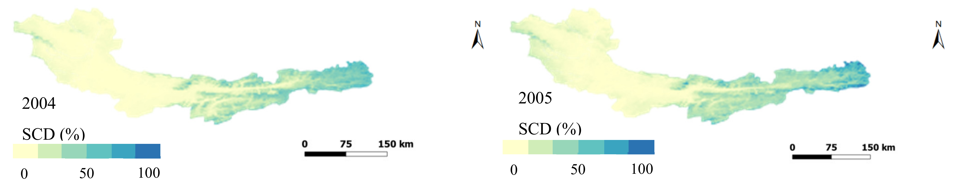
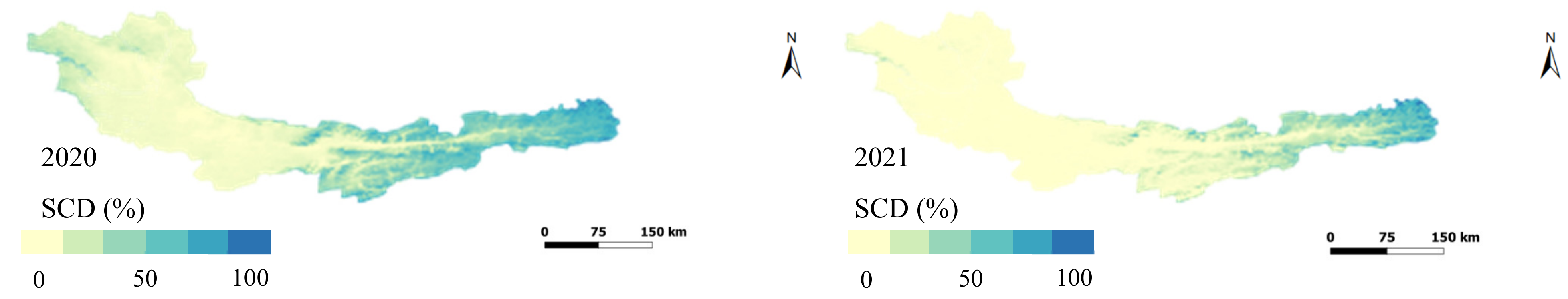
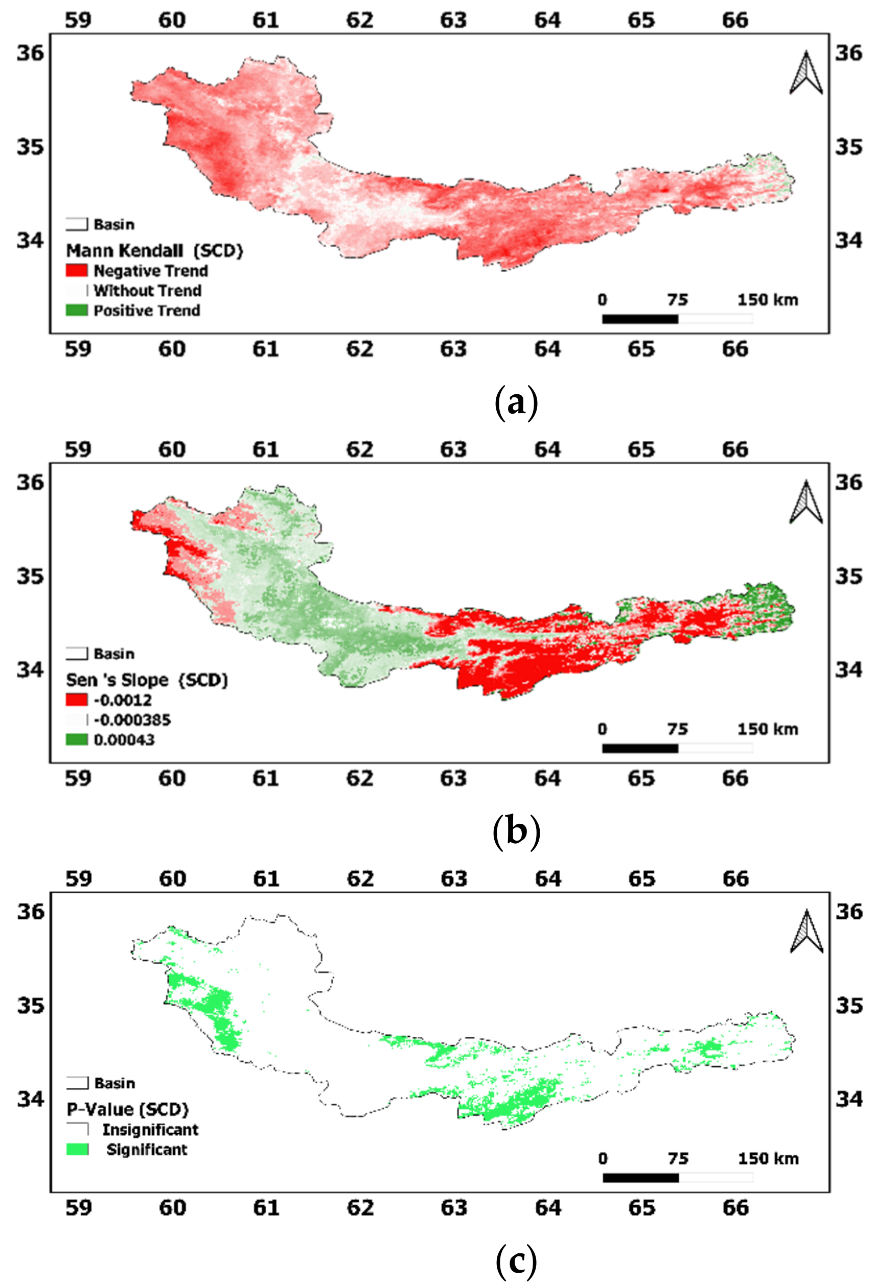
3.5. Spatio-Temporal Distribution Annual Snow Cover Duration from MODIS in the Doosti Dam’s Basin (2004–2021)

In areas with higher elevations, the MODIS/Terra sensor has ample capability to detect SCD. The MODIS/Terra 8-day snow cover product (MOD10A1) was used to monitor the SCD maps in the Doosti Dam’s river basin (Figure 11). The effects of elevation on annual SCD for the period of 2004–2021 was observed in this figure as lower elevation regions experienced less snow cover throughout the period.

The SCD varied from zero to nearer 100 % and followed the topography. Figure 10 indicates the variation of snow pixel numbers (SPN) as an indicator of SCE and in the region and the extent of Doosti Dam’s reservoir for the period of 2004 to 2021. Maximum SCD occurred in the high elevated areas (50%). Although statistically insignificant, it indicates that the yearly snow cover generally decreased somewhat at higher elevations and remained constant at lower elevations (approximately 20%). The whole basin (especially the mountainous areas) received the SCD (50%) in the year 2008.

Figure 12 shows the spatial distribution of trends in the annual evapotranspiration based on MOD10A1 estimates for the period from 2004 to 2021. The spatial pattern of the MK test shows that snow cover duration had no significant trend in a large area of the basin (Figure 12a) and in Figure 12c no trend was identified for most of Doosti Dam’s basin; however, the significant trend was recognised upstream.

Figure 12b shows a decreasing trend for SCD in the western part of the basin with a Sen’s slope calculation of −0.0012 (lower limit) indicating a downward trend for the significant tendencies at a 95% confidence level.

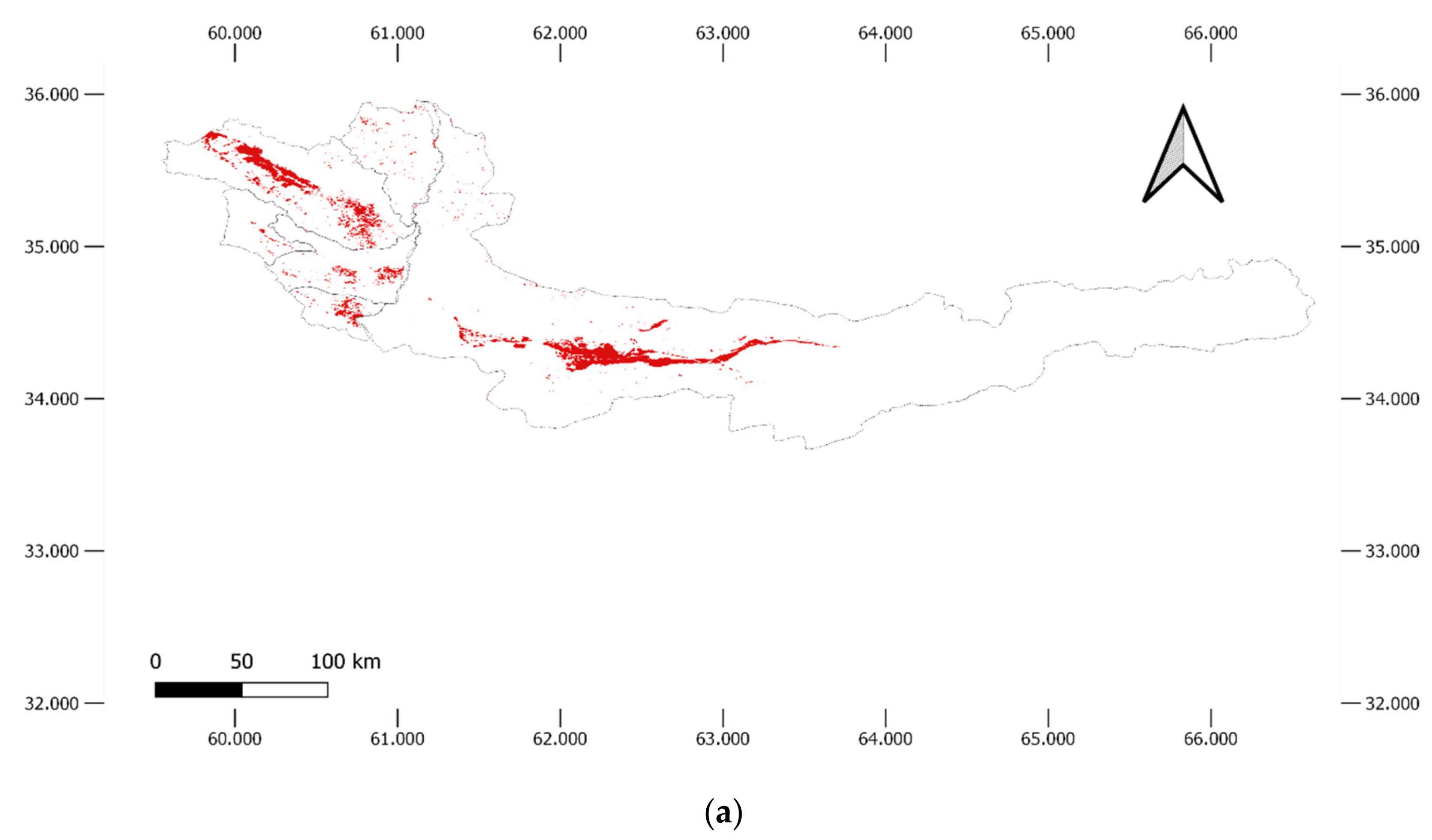
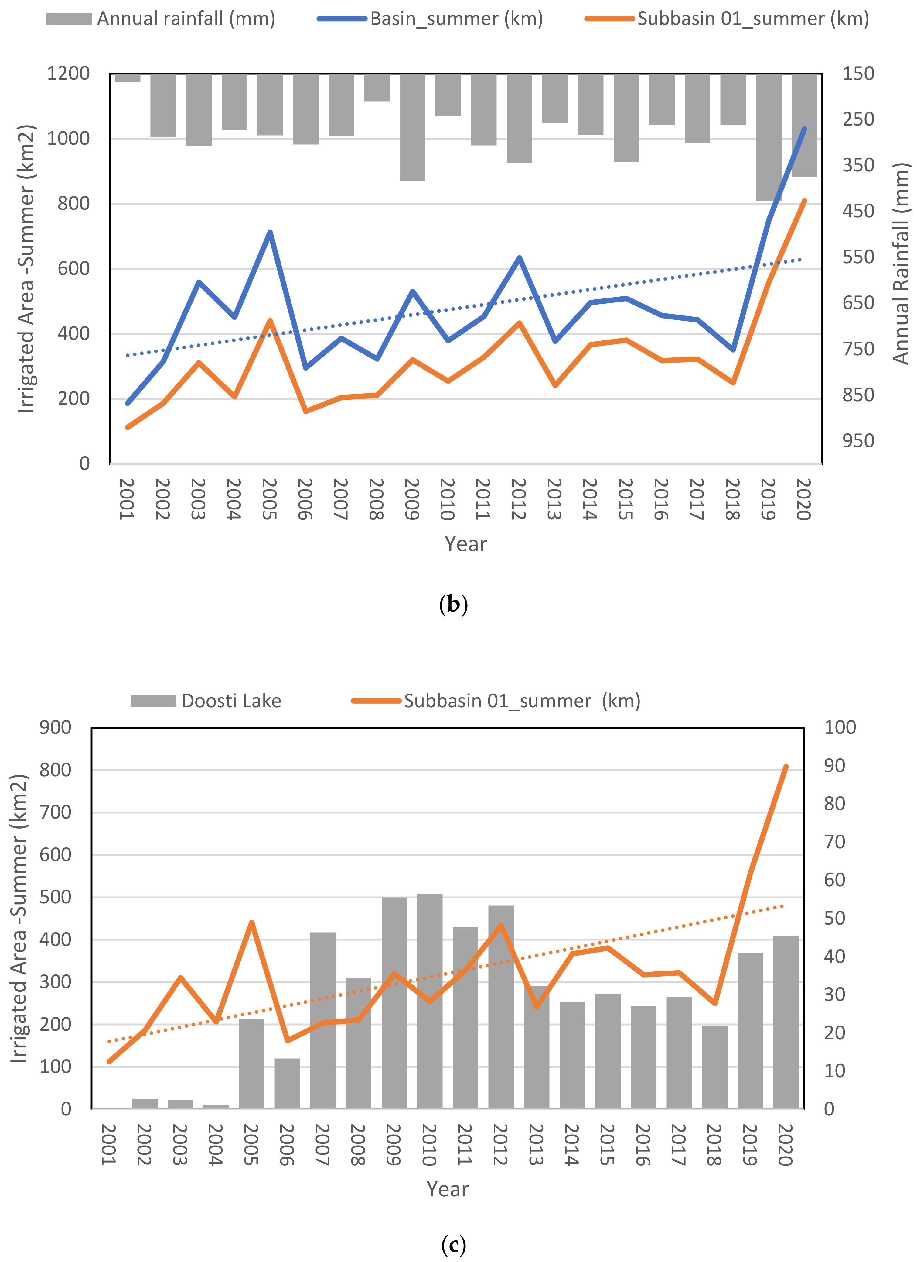
3.6. Spatio-Temporal Distribution for Summer Irrigated Cultivated Areas in the Doosti Dam Basin (2001–2021)

The map presented in Figure 13 shows the irrigated cultivated areas for the summer growing season. Figure 13a demonstrates that irrigated land predominates in the water management region along the Doosti Dam’s river. The dominance of the irrigated region supports the fact that irrigation receives most of the freshwater resources available. The irrigated cultivated areas in both the winter and summer growing seasons were extracted by deriving the maximum NDVI maps in the winter (APR–JUN) and summer (JUL–SEP) growing seasons and applying threshold values to the NDVI maps and elevation from Doosti Dam’s river basin baseline. It also shows that the downstream and river line in the centre identify irrigated areas.

Figure 13b illustrates the strong correlation between irrigated areas in summer and precipitation. The cultivated areas increased from 451 km² to 1029 km² as a result of increase in rainfall from 272 mm to 375 mm during 2004 to 2020. This increase does not necessarily indicate a change in the amount of land irrigated; it just indicates that certain agricultural areas that were not irrigated before 2017 were irrigated in 2018. Agriculture’s status as a vital industry in the basin, permitting it to continue working throughout the COVID-19 pandemic lockdown period, is the key contributing factor in the increases in the irrigated area in 2020. Since many individuals lost their other means of income during lockdown, agriculture emerged as a substitute.

It is worth mentioning that the cultivated areas ranging from 2001 to 2020 containing three months of data for summer and winter are from January to January, respectively. From Figure 13b, it can be seen that in the periods from 2001 to 2005, the cultivated areas tripled from 200 km² to 600 km² and between 2006 and 2018, the cultivated areas fluctuated. Between 2006 and 2018, high rainfall in 2009 (343 mm) and 2012 (384 mm) exhibited an increase in the cultivated areas for the basin and subbasin from 320 km² to 530 km² in 2009 and, 430 km² to 630 km² in 2012, respectively. Moreover, irrigated areas witnessed a sharp increase for the basin and subbasin which varied from 350 km² (2018) to 1029 km² (2020) and from 250 km² (2018) to 800 km² (2020), respectively.

Figure 13c shows a significant ascending trend in the irrigated areas in the summer season which is an indicator of an increase or densification of vegetation cover in this region. Interestingly, both the irrigated areas and Doosti Dam’s Lake showed an identical trend for the highest increase for the year 2006 (320 km²) and (56 km²), and the year 2020 (800 km²) and (45 km²), respectively. This also confirmed that whole basin experienced an increase in irrigated areas alongside the Doosti Lake.

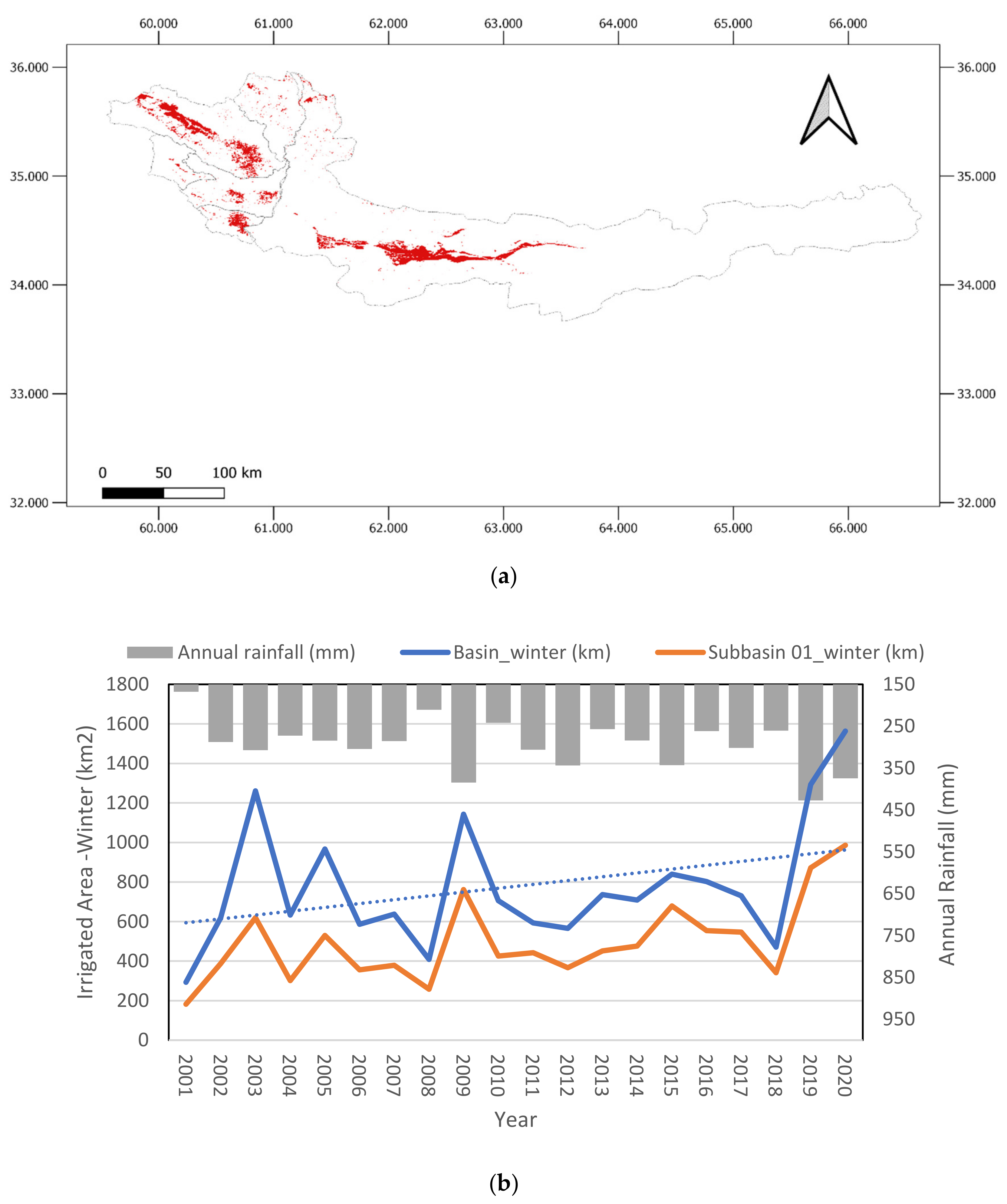
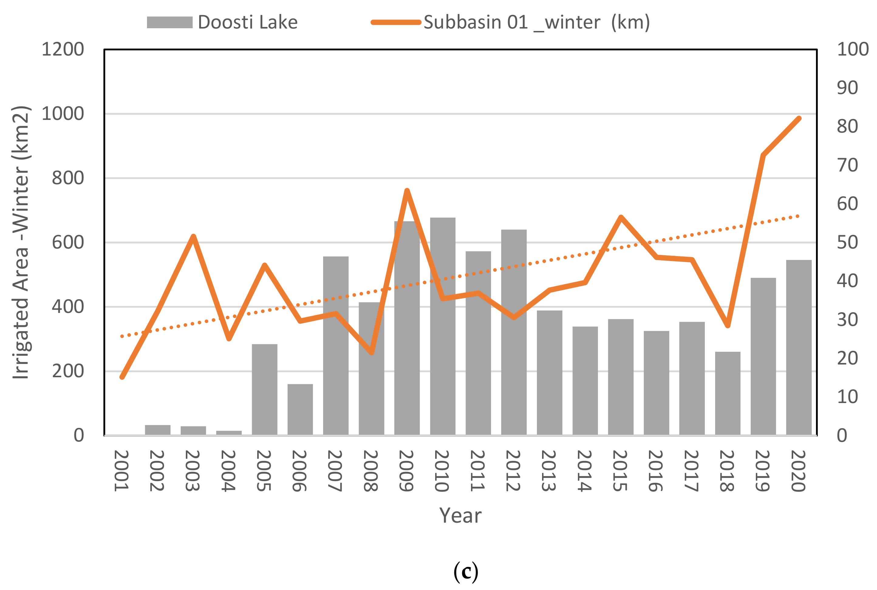
3.7. Spatio-Temporal Distribution Winter Irrigated Cultivated Areas in the Doosti Dam Basin’s (2001–2020)

The map presented in Figure 14 shows the irrigated cultivated areas for the winter growing season. Figure 14a illustrates that irrigated land predominated in the water management region. During the winter season, the cultivated areas increased from 632 km² to 1563 km² as a result of increased rainfall from 273 mm to 400 mm over the period 2004 to 2020 (Figure 14b). Figure 14c represents a sharp ascending trend in the irrigated areas in the winter season, which is an indicator of an increase in cultivated areas along the Doosti Dam Lake. The irrigated areas and Doosti Dam’s Lake showed similar trends with the highest increase in the year 2020 (985 km²) and (45 km²) over the 20 years, respectively.

Although the irrigated areas in the winter growing season were significantly higher compared to the summer season, the trend of changes in the cultivated areas from 2011 to 2018 was not significant (Figure 13b and 14b).

4. Discussion

Using three-gauge measurements and multi-hydroclimatic gridded datasets at various elevation ranges (from 278 m to 4163 m), this study analyses trends and spatiotemporal variability in multi-hydroclimatic variables over the past two decades. A significant increasing trend in precipitation is apparent over the eastern regions of Iran leading to a positive annual trend over the pixels [30]. Unlike the findings of previous studies [37,65], temperature demonstrated a slight decrease, which might be as a result of the different research periods and various precipitation dataset types (point and pixel-based) employed for trend analysis. Indeed, while a satellite product calculates precipitation variables across a region, a rain gauge measures variables at a particular location [30]. The investigation of the trends of evapotranspiration indicated the positive increasing trend over the regions of Iran, confirming the results of a previous study in Iran [66].

Snow cover generally declined slightly over the period 2004–2021, higher elevation areas experienced an increase in SCA alongside a declining temperature trend [67,68]. Land-use changes and the construction of dams, reservoirs and irrigation canals have been identified as the primary anthropogenic activities causing variations in runoff [69]. Irrigated areas in both the winter (APR-JUN) and summer (JUL-SEP) growing seasons increased through the nonparametric tests across the basin. Human activities increased the irrigated areas and so are considered to be the most significant possible driver of the diversion of runoff in the basin [69]. The results also confirmed that the strong correlation between precipitation and irrigated areas and both irrigated areas and the Doosti lake showed an identical trend.

The GEE platform has two advantages: (1) due to data limitations in the inaccessible, sparsely gauged basin, it facilitated data collection in some regions which have few weather stations and (2) it enabled us to process and analyse numerous hydroclimatic variables, including land use, snow cover, lake reservoir, evapotranspiration, integrating the publicly available big geospatial data.

Considering the spatiotemporal variability of numerous hydroclimatic variables in data-sparse regions, this research provides insights for the policy-maker seeking mitigation strategies. On the other hand, the lack of access to long-term data of consistently high quality, missing data and data with inadequate spatial and temporal coverage could have a detrimental impact, leading to poor decision making. The absence of in situ measurements for other hydroclimatic variables, in addition to temperature and precipitation, is another limitation of this study.

As we only covered the trends with the MK and Sen’s slope, investigating season–trend fit models such as antileakage least-squares spectral analysis [70,71,72] or least absolute shrinkage and selection operator (LASSO) [73] is recommended. The Mann–Kendall test’s essential requirement is that the data should be independent and mostly applied to an annual-scale time series [30,37,61]. Therefore, before applying the Mann–Kendall test, any positive or negative autocorrelation of the data should be removed [74]. Moreover, in this research, Mann–Kendall was applied to annual-scale time series, so seasonality is not present in annual-scale time series. However, prior to annual trend analysis, the autocorrelation test was applied to ensure that there was no seasonality present and to eliminate any existence of an autocorrelation impact on the data [75]. Furthermore, probable changes in the future are generally studied by general circulation models (GCMs) [76,77,78] and scenarios [79,80]. However, climate projections are uncertain for the detection of extremes [81]. The probable changes in environmental flow release can be assessed by applying the downscaled outputs of multi-GCMs forced into hydrological models [82] under a non-stationary assumption [83], which can be further studied in the future. Hence, study under non-stationary assumptions to reduce the damage caused by climate change and human activities is suggested.

5. Conclusions

Given the high spatial and temporal variations in hydroclimatic variables in transboundary regions, it is necessary for water resource decision-makers to understand the hydroclimatic behaviours through the analysis of the variables’ heterogenicity. This study investigated the spatiotemporal aspects of numerous hydroclimatic variables based on GEE at the transboundary level. The nonparametric statistical tests (MK and Sen’s slope) were applied coupled with an advanced web-based cloud computing platform (GEE) to delineate the monotonic trend of data. This study provides a comprehensive understanding of the long-term trend of hydroclimatic variables. The spatial and temporal changes of hydrometeorological temperature (MODIS-Terra), evapotranspiration (MODIS-Terra), snow cover distribution (MODIS-Terra), MODIS Terra NDVI in relation to precipitation (CHIRPS), topography (DEM SRTM) and the LANDSAT NDWI index in the Doosti Dam’s basin are presented for the period 2004 to 2021. The key findings of this study are as below:

(1)

The study showed how well multisensory satellite data can be used to predict hydrometeorological spatiotemporal trends, especially in transboundary high elevation areas when accessing station-observed data is a major challenge. It demonstrated that, for most variables, these trends largely relied on elevation. This statistically upward trend was seen in rainfall, evapotranspiration, and lower temperature during the years 2004 to 2021, but did not have a remarkable effect on snow cover duration.

(2)

This study was focused on understanding how the irrigated cultivated lands responded to different hydroclimatic variables. Because it is a transboundary region, has diverse topography and climate change conditions, the monitoring of the irrigated lands was difficult. Elevation had a significant influence on the climate and the Doosti Dam, situated at a lower elevation, was employed to comprehend the long-term spatiotemporal variability of the irrigated areas and related climatic and hydrological causes. NDVI derived from MODIS indicated the strong correlation between the NDVI and precipitation in the winter.

(3)

Additionally, the findings demonstrate that GEE is an effective method for compiling and establishing the spatiotemporal fluctuations in various variables and that remotely sensed data products consistently represent ground observations in remote transboundary areas. It is anticipated that the socio-ecological system in this transboundary area would decline owing to unsustainable water management which will negatively affect the conditions of the residents. It is important to consider the environmental right of the lakes to improve the conditions in the transboundary river basin. GEE’s potential has not yet been fully realised, despite the fact that it has gradually evolved into a platform for remote sensing research. With the help of GEE, this study offers a rapid and feasible method for determining spatiotemporal climatic trends. The methodology can be easily applied to other areas with comparable issues when combined with the tools made available by GEE. The results of this study can aid in the management of water resources and the preservation of the ecological environment in the Doosti Dam’s basin and other transboundary regions.

(4)

In an area characterised by a complicated set of interactions between precipitation, evapotranspiration, temperature, NDVI, snow cover, lake area and discharge, the overall findings of this study could guide water resource management strategies. Future research should take these elements into account in order to provide a full forecast of the spatiotemporal climatic dynamics of transboundary areas, especially in light of the current period of rapid climate change (both natural and anthropogenic).

References

- Mianabadi, H.; Alioghli, S.; Morid, S. Quantitative evaluation of ‘No-harm’rule in international transboundary water law in the Helmand River Basin. J. Hydrol. 2021, 599, 126368. [Google Scholar] [CrossRef]
- Al-Faraj, F.A.; Scholz, M. Assessment of temporal hydrologic anomalies coupled with drought impact for a transboundary river flow regime: The Diyala watershed case study. J. Hydrol. 2014, 517, 64–73. [Google Scholar] [CrossRef]
- Wu, J.; Liu, Z.; Yao, H.; Chen, X.; Chen, X.; Zheng, Y.; He, Y. Impacts of reservoir operations on multi-scale correlations between hydrological drought and meteorological drought. J. Hydrol. 2018, 563, 726–736. [Google Scholar] [CrossRef]
- Gao, H.; Birkett, C.; Lettenmaier, D.P. Global monitoring of large reservoir storage from satellite remote sensing. Water Resour. Res. 2012, 48, 1–12. [Google Scholar] [CrossRef]
- Moreno, M.; Bertolín, C.; Ortiz, P.; Ortiz, R. Satellite product to map drought and extreme precipitation trend in Andalusia, Spain: A novel method to assess heritage landscapes at risk. Int. J. Appl. Earth Obs. Geoinf. 2022, 110, 102810. [Google Scholar] [CrossRef]
- Pakdel Khasmakhi, H.; Vazifedoust, M.; Marofi, S.; Tizro, A.T. Simulation of river discharge in ungauged catchments by forcing GLDAS products to a hydrological model (a case study: Polroud basin, Iran). Water Supply 2020, 20, 277–286. [Google Scholar] [CrossRef]
- Sadeghi Loyeh, N.; Massah Bavani, A. Daily maximum runoff frequency analysis under non-stationary conditions due to climate change in the future period: Case study Ghareh Sou Basin. J. Water Clim. Chang. 2021, 12, 1910–1929. [Google Scholar] [CrossRef]
- Erazo, B.; Bourrel, L.; Frappart, F.; Chimborazo, O.; Labat, D.; Dominguez-Granda, L.; Matamoros, D.; Mejia, R. Validation of satellite estimates (Tropical Rainfall Measuring Mission, TRMM) for rainfall variability over the Pacific slope and Coast of Ecuador. Water 2018, 10, 213. [Google Scholar] [CrossRef]
- Ma, L.; Liu, Y.; Zhang, X.; Ye, Y.; Yin, G.; Johnson, B.A. Deep learning in remote sensing applications: A meta-analysis and review. ISPRS J. Photogramm. Remote Sens. 2019, 152, 166–177. [Google Scholar] [CrossRef]
- Ellsäßer, F.; Röll, A.; Stiegler, C.; Hölscher, D. Introducing QWaterModel, a QGIS plugin for predicting evapotranspiration from land surface temperatures. Environ. Model. Softw. 2020, 130, 104739. [Google Scholar] [CrossRef]
- Zaki, A.; Buchori, I.; Sejati, A.W.; Liu, Y. An object-based image analysis in QGIS for image classification and assessment of coastal spatial planning. Egypt. J. Remote Sens. Space Sci. 2022, 25, 349–359. [Google Scholar] [CrossRef]
- Wang, C.; Jia, M.; Chen, N.; Wang, W. Long-term surface water dynamics analysis based on Landsat imagery and the Google Earth Engine platform: A case study in the middle Yangtze River Basin. Remote Sens. 2018, 10, 1635. [Google Scholar] [CrossRef]
- Dastour, H.; Ghaderpour, E.; Hassan, Q.K. A combined approach for monitoring monthly surface water/ice dynamics of Lesser Slave Lake via Earth observation data. IEEE J. Sel. Top. Appl. Earth Obs. Remote Sens. 2022, 15, 6402–6417. [Google Scholar] [CrossRef]
- Gorelick, N.; Hancher, M.; Dixon, M.; Ilyushchenko, S.; Thau, D.; Moore, R. Google Earth Engine: Planetary-scale geospatial analysis for everyone. Remote Sens. Environ. 2017, 202, 18–27. [Google Scholar] [CrossRef]
- Tamiminia, H.; Salehi, B.; Mahdianpari, M.; Quackenbush, L.; Adeli, S.; Brisco, B. Google Earth Engine for geo-big data applications: A meta-analysis and systematic review. ISPRS J. Photogramm. Remote Sens. 2020, 164, 152–170. [Google Scholar] [CrossRef]
- Google Developers: Get Started with Earth Engine. Available online: https://developers.google.com/earth-engine/getstarted (accessed on 21 September 2022).
- Mozafari, M.; Raeisi, E.; Zare, M. Water leakage paths in the Doosti Dam, Turkmenistan and Iran. Environ. Earth Sci. 2012, 65, 103–117. [Google Scholar] [CrossRef]
- Majidi, M.; Alizadeh, A.; Farid, A.; Vazifedoust, M. Estimating evaporation from lakes and reservoirs under limited data condition in a semi-arid region. Water Resour. Manag. 2015, 29, 3711–3733. [Google Scholar] [CrossRef]
- Rezaei Sekkeravani, D.; Chenari, S.; Faraji, M.; Dashti, s.F. Study the Iranian hydropolitical challenges in the shared drainage basins with Neighboring Countries. IOSR J. Humanit. Soc. Sci. IOSR-JHSS 2018, 23, 67–78. [Google Scholar] [CrossRef]
- Akbari, M.; Mirchi, A.; Roozbahani, A.; Gafurov, A.; Kløve, B.; Haghighi, A.T. Desiccation of the transboundary Hamun Lakes between Iran and Afghanistan in response to hydro-climatic droughts and anthropogenic activities. J. Great Lakes Res. 2022, 48, 876–889. [Google Scholar] [CrossRef]
- Salomon, J.; Hodges, J.C.; Friedl, M.; Schaaf, C.; Strahler, A.; Gao, F.; Schneider, A.; Zhang, X.; El Saleous, N.; Wolfe, R.E. Global land-water mask derived from MODIS Nadir BRDF-adjusted reflectances (NBAR) and the MODIS land cover algorithm. In Proceedings of the IGARSS 2004. 2004 IEEE International Geoscience and Remote Sensing Symposium, Anchorage, AK, USA, 20–24 September 2004. [Google Scholar]
- Li, L.; Vrieling, A.; Skidmore, A.; Wang, T.; Turak, E. Monitoring the dynamics of surface water fraction from MODIS time series in a Mediterranean environment. Int. J. Appl. Earth Obs. Geoinf. 2018, 66, 135–145. [Google Scholar] [CrossRef]
- Carroll, M.; Wooten, M.; DiMiceli, C.; Sohlberg, R.; Kelly, M. Quantifying surface water dynamics at 30 m spatial resolution in the North American high northern latitudes 1991–2011. Remote Sens. 2016, 8, 622. [Google Scholar] [CrossRef]
- Pekel, J.-F.; Cottam, A.; Gorelick, N.; Belward, A.S. High-resolution mapping of global surface water and its long-term changes. Nature 2016, 540, 418–422. [Google Scholar] [CrossRef] [PubMed]
- Tulbure, M.G.; Broich, M.; Stehman, S.V.; Kommareddy, A. Surface water extent dynamics from three decades of seasonally continuous Landsat time series at subcontinental scale in a semi-arid region. Remote Sens. Environ. 2016, 178, 142–157. [Google Scholar] [CrossRef]
- Shen, G.; Fu, W.; Guo, H.; Liao, J. Water Body Mapping Using Long Time Series Sentinel-1 SAR Data in Poyang Lake. Water 2022, 14, 1902. [Google Scholar] [CrossRef]
- Surface Water Changes. (1985–2016). Available online: http://aqua-monitor.deltares.nl (accessed on 21 September 2022).
- Donchyts, G.; Baart, F.; Winsemius, H.; Gorelick, N.; Kwadijk, J.; Van De Giesen, N. Earth’s surface water change over the past 30 years. Nat. Clim. Chang. 2016, 6, 810–813. [Google Scholar] [CrossRef]
- Gholizadeh Sarabi, S.; Rahnama, M.R. From self-sufficient provision of water and energy to regenerative urban development and sustainability: Exploring the potentials in Mashhad City, Iran. J. Environ. Plan. Manag. 2021, 64, 2459–2480. [Google Scholar] [CrossRef]
- Mosaffa, H.; Sadeghi, M.; Hayatbini, N.; Afzali Gorooh, V.; Akbari Asanjan, A.; Nguyen, P.; Sorooshian, S. Spatiotemporal variations of precipitation over Iran using the high-resolution and nearly four decades satellite-based PERSIANN-CDR dataset. Remote Sens. 2020, 12, 1584. [Google Scholar] [CrossRef]
- Raziei, T.; Daryabari, J.; Bordi, I.; Modarres, R.; Pereira, L.S. Spatial patterns and temporal trends of daily precipitation indices in Iran. Clim. Chang. 2014, 124, 239–253. [Google Scholar] [CrossRef]
- Luo, R.; Yuan, Q.; Yue, L.; Shi, X. Monitoring recent lake variations under climate change around the Altai mountains using multimission satellite data. IEEE J. Sel. Top. Appl. Earth Obs. Remote Sens. 2020, 14, 1374–1388. [Google Scholar] [CrossRef]
- Veh, G.; Korup, O.; Roessner, S.; Walz, A. Detecting Himalayan glacial lake outburst floods from Landsat time series. Remote Sens. Environ. 2018, 207, 84–97. [Google Scholar] [CrossRef]
- Ma, Y.; Xu, N.; Sun, J.; Wang, X.H.; Yang, F.; Li, S. Estimating water levels and volumes of lakes dated back to the 1980s using Landsat imagery and photon-counting lidar datasets. Remote Sens. Environ. 2019, 232, 111287. [Google Scholar] [CrossRef]
- Lu, S.; Ouyang, N.; Wu, B.; Wei, Y.; Tesemma, Z. Lake water volume calculation with time series remote-sensing images. Int. J. Remote Sens. 2013, 34, 7962–7973. [Google Scholar] [CrossRef]
- Moghim, S. Impact of climate variation on hydrometeorology in Iran. Glob. Planet. Chang. 2018, 170, 93–105. [Google Scholar] [CrossRef]
- Malaekeh, S.; Safaie, A.; Shiva, L.; Tabari, H. Spatio-temporal variation of hydro-climatic variables and extreme indices over Iran based on reanalysis data. Stoch. Environ. Res. Risk Assess. 2022, 1–28. [Google Scholar] [CrossRef]
- Arnell, N.W.; Gosling, S.N. The impacts of climate change on river flow regimes at the global scale. J. Hydrol. 2013, 486, 351–364. [Google Scholar] [CrossRef]
- Blum, J.R.; Eichhorn, A.; Smith, S.; Sterle-Contala, M.; Cooperstock, J.R. Real-time emergency response: Improved management of real-time information during crisis situations. J. Multimodal User Interfaces 2014, 8, 161–173. [Google Scholar] [CrossRef]
- Irwin, K.; Beaulne, D.; Braun, A.; Fotopoulos, G. Fusion of SAR, optical imagery and airborne LiDAR for surface water detection. Remote Sens. 2017, 9, 890. [Google Scholar] [CrossRef]
- Li, Z.-L.; Tang, B.-H.; Wu, H.; Ren, H.; Yan, G.; Wan, Z.; Trigo, I.F.; Sobrino, J.A. Satellite-derived land surface temperature: Current status and perspectives. Remote Sens. Environ. 2013, 131, 14–37. [Google Scholar] [CrossRef]
- Li, S.; Yu, Y.; Sun, D.; Tarpley, D.; Zhan, X.; Chiu, L. Evaluation of 10 year AQUA/MODIS land surface temperature with SURFRAD observations. Int. J. Remote Sens. 2014, 35, 830–856. [Google Scholar] [CrossRef]
- Wan, Z. Collection-5 MODIS Land Surface Temperature Products Users’ Guide. ICESS, University of California, Santa Barbara. 2007. Available online: https://www.cen.uni-hamburg.de/en/icdc/data/land/docs-land/modis-lst-products-user-guide-c5.pdf (accessed on 21 September 2022).
- MOD11A1. Available online: https://developers.google.com/earth-engine/datasets/catalog/MODIS_061_MOD11A1 (accessed on 21 September 2022).
- Dietz, A.J.; Kuenzer, C.; Gessner, U.; Dech, S. Remote sensing of snow–a review of available methods. Int. J. Remote Sens. 2012, 33, 4094–4134. [Google Scholar] [CrossRef]
- MOD10A1. Available online: https://developers.google.com/earth-engine/datasets/catalog/MODIS_006_MOD10A1 (accessed on 21 September 2022).
- MOD09GQ. Available online: https://developers.google.com/earth-engine/datasets/catalog/MODIS_061_MOD09GQ (accessed on 21 September 2022).
- Running, S.; Mu, Q.; Zhao, M. MOD16A2 MODIS/Terra Net Evapotranspiration 8-day L4 global 500m SIN Grid V006 [Data Set]. NASA EOSDIS Land Processes DAAC; 2017. Available online: https://ladsweb.modaps.eosdis.nasa.gov/missions-and-measurements/products/MOD16A2 (accessed on 21 September 2022).
- Tian, H.; Li, W.; Wu, M.; Huang, N.; Li, G.; Li, X.; Niu, Z. Dynamic monitoring of the largest freshwater lake in China using a new water index derived from high spatiotemporal resolution Sentinel-1A data. Remote Sens. 2017, 9, 521. [Google Scholar] [CrossRef]
- Plug, L.J.; Walls, C.; Scott, B. Tundra lake changes from 1978 to 2001 on the Tuktoyaktuk Peninsula, Western Canadian Arctic. Geophys. Res. Lett. 2008, 35. [Google Scholar] [CrossRef]
- Tao, S.; Fang, J.; Zhao, X.; Zhao, S.; Shen, H.; Hu, H.; Tang, Z.; Wang, Z.; Guo, Q. Rapid loss of lakes on the Mongolian Plateau. Proc. Natl. Acad. Sci. USA 2015, 112, 2281–2286. [Google Scholar] [CrossRef] [PubMed]
- Du, Z.; Bin, L.; Ling, F.; Li, W.; Tian, W.; Wang, H.; Gui, Y.; Sun, B.; Zhang, X. Estimating surface water area changes using time-series Landsat data in the Qingjiang River Basin, China. J. Appl. Remote Sens. 2012, 6, 063609. [Google Scholar] [CrossRef]
- Xu, H. Modification of normalised difference water index (NDWI) to enhance open water features in remotely sensed imagery. Int. J. Remote Sensing. 2006, 27, 3025–3033. [Google Scholar] [CrossRef]
- Pham-Duc, B.; Prigent, C.; Aires, F. Surface water monitoring within Cambodia and the Vietnamese Mekong Delta over a year, with Sentinel-1 SAR observations. Water 2017, 9, 366. [Google Scholar] [CrossRef]
- Li, W.; Du, Z.; Ling, F.; Zhou, D.; Wang, H.; Gui, Y.; Sun, B.; Zhang, X. A comparison of land surface water mapping using the normalized difference water index from TM, ETM+ and ALI. Remote Sens. 2013, 5, 5530–5549. [Google Scholar] [CrossRef]
- Gorelick, N.; Clinton, N. Multitemporal Supervised Classification Using Google Earth Engine. In Proceedings of the AGU Fall Meeting, Washington, DC, USA, 10–14 December 2018. [Google Scholar]
- Banerjee, A.; Chen, R.; Meadows, M.E.; Singh, R.; Mal, S.; Sengupta, D. An analysis of long-term rainfall trends and variability in the uttarakhand himalaya using Google Earth Engine. Remote Sens. 2020, 12, 709. [Google Scholar] [CrossRef]
- Mann, H.B. Nonparametric tests against trend. Econom. J. Econom. Soc. 1945, 13, 245–259. [Google Scholar] [CrossRef]
- Kendall, M. Rank Correlation Methods, 4th ed.; Charles Griffin: London, UK, 1975. [Google Scholar]
- Zolghadr-Asli, B.; Bozorg-Haddad, O.; Sarzaeim, P.; Chu, X. Investigating the variability of GCMs’ simulations using time series analysis. J. Water Clim. Change 2019, 10, 449–463. [Google Scholar] [CrossRef]
- Tabari, H.; Marofi, S.; Aeini, A.; Talaee, P.H.; Mohammadi, K. Trend analysis of reference evapotranspiration in the western half of Iran. Agric. For. Meteorol. 2011, 151, 128–136. [Google Scholar] [CrossRef]
- Gholami, H.; Moradi, Y.; Lotfirad, M.; Gandomi, M.A.; Bazgir, N.; Shokrian Hajibehzad, M. Detection of abrupt shift and non-parametric analyses of trends in runoff time series in the Dez river basin. Water Supply 2022, 22, 1216–1230. [Google Scholar] [CrossRef]
- Sen, P.K. Estimates of the regression coefficient based on Kendall’s tau. J. Am. Stat. Assoc. 1968, 63, 1379–1389. [Google Scholar] [CrossRef]
- Banerjee, A.; Chen, R.; Meadows, M.E.; Sengupta, D.; Pathak, S.; Xia, Z.; Mal, S. Tracking 21st century climate dynamics of the Third Pole: An analysis of topo-climate impacts on snow cover in the central Himalaya using Google Earth Engine. Int. J. Appl. Earth Obs. Geoinformation. 2021, 103, 102490. [Google Scholar] [CrossRef]
- Tabari, H.; Somee, B.S.; Zadeh, M.R. Testing for long-term trends in climatic variables in Iran. Atmos. Res. 2011, 100, 132–140. [Google Scholar] [CrossRef]
- Alizadeh-Choobari, O.; Najafi, M. Extreme weather events in Iran under a changing climate. Clim. Dyn. 2018, 50, 249–260. [Google Scholar] [CrossRef]
- Bilal, H.; Chamhuri, S.; Mokhtar, M.B.; Kanniah, K.D. Recent snow cover variation in the upper Indus Basin of Gilgit Baltistan, Hindukush Karakoram Himalaya. J. Mt. Sci. 2019, 16, 296–308. [Google Scholar] [CrossRef]
- Azmat, M.; Liaqat, U.W.; Qamar, M.U.; Awan, U.K. Impacts of changing climate and snow cover on the flow regime of Jhelum River, Western Himalayas. Reg. Environ. Change 2017, 17, 813–825. [Google Scholar] [CrossRef]
- Yang, Y.; Tian, F. Abrupt change of runoff and its major driving factors in Haihe River Catchment, China. J. Hydrol. 2009, 374, 373–383. [Google Scholar] [CrossRef]
- Hui, Y.; Pagiatakis, S. Least squares spectral analysis and its application to superconducting gravimeter data analysis. Geo-Spat. Inf. Sci. 2004, 7, 279–283. [Google Scholar] [CrossRef]
- Mathias, A.; Grond, F.; Guardans, R.; Seese, D.; Canela, M.; Diebner, H.H. Algorithms for spectral analysis of irregularly sampled time series. J. Stat. Softw. 2004, 11, 1–27. [Google Scholar] [CrossRef]
- Ghaderpour, E. Multichannel antileakage least-squares spectral analysis for seismic data regularization beyond aliasing. Acta Geophys. 2019, 67, 1349–1363. [Google Scholar] [CrossRef]
- Ghaderpour, E.; Vujadinovic, T.; Hassan, Q.K. Application of the least-squares wavelet software in hydrology: Athabasca River basin. J. Hydrol. Reg. Stud. 2021, 36, 100847. [Google Scholar] [CrossRef]
- Sa’adi, Z.; Shahid, S.; Ismail, T.; Chung, E.-S.; Wang, X.-J. Trends analysis of rainfall and rainfall extremes in Sarawak, Malaysia using Modified Mann–Kendall test. Meteorol. Atmos. Phys. 2019, 131, 263–277. [Google Scholar] [CrossRef]
- Lacombe, G.; Mccartney, M.; Forkuor, G. Drying climate in Ghana over the period 1960–2005: Evidence from the resampling-based Mann-Kendall test at local and regional levels. Hydrol. Sci. J. 2012, 57, 1594–1609. [Google Scholar] [CrossRef]
- Tofiq, F.; Güven, A. Potential changes in inflow design flood under future climate projections for Darbandikhan Dam. J. Hydrol. 2015, 528, 45–51. [Google Scholar] [CrossRef]
- Alfieri, L.; Bisselink, B.; Dottori, F.; Naumann, G.; de Roo, A.; Salamon, P.; Wyser, K.; Feyen, L. Global projections of river flood risk in a warmer world. Earth’s Future 2017, 5, 171–182. [Google Scholar] [CrossRef]
- Zolghadr-Asli, B.; Bozorg-Haddad, O.; Enayati, M.; Goharian, E. Developing a robust multi-attribute decision-making framework to evaluate performance of water system design and planning under climate change. Water Resour. Manag. 2021, 35, 279–298. [Google Scholar] [CrossRef]
- Yin, J.; Guo, S.; Yang, Y.; Chen, J.; Gu, L.; Wang, J.; He, S.; Wu, B.; Xiong, J. Projection of droughts and their socioeconomic exposures based on terrestrial water storage anomaly over China. Sci. China Earth Sci. 2022, 65, 1772–1787. [Google Scholar] [CrossRef]
- Zolghadr-Asli, B.; Bozorg-Haddad, O.; Chu, X. Effects of the uncertainties of climate change on the performance of hydropower systems. J. Water Clim. Chang. 2019, 10, 591–609. [Google Scholar] [CrossRef]
- Salas, J.; Obeysekera, J.; Vogel, R. Techniques for assessing water infrastructure for nonstationary extreme events: A review. Hydrol. Sci. J. 2018, 63, 325–352. [Google Scholar] [CrossRef]
- Yin, J.; Guo, S.; Gu, L.; Zeng, Z.; Liu, D.; Chen, J.; Shen, Y.; Xu, C.-Y. Blending multi-satellite, atmospheric reanalysis and gauge precipitation products to facilitate hydrological modelling. J. Hydrol. 2021, 593, 125878. [Google Scholar] [CrossRef]
- Cheng, L.; AghaKouchak, A. Nonstationary precipitation intensity-duration-frequency curves for infrastructure design in a changing climate. Sci. Rep. 2014, 4, 1. [Google Scholar] [CrossRef] [PubMed]