The Optical Model Absorption Term in the Frame of Fractional Derivatives

Abstract

The complex optical model has been widely used to describe the elastic scattering of the nucleon–nucleus. The imaginary term of the optical potential takes into account the non-elastic scattering processes. This term was taken to be a Woods–Saxon form factor or its derivative to simulate the volume absorption or the absorption localized at the surface of the target, respectively. In this study, a fractional derivative of the Woods–Saxon potential with $0<\alpha <1$ was used, where $\alpha =0$ and $\alpha =1$ give the volume and the surface absorption form factor, respectively.

1. Introduction

In the center-of-mass frame, the Schrodinger equation simplifies the nucleon–nucleus scattering problem to a particle scattered from a potential. This potential is considered to be a complex one, with the real part describing elastic scattering processes and the imaginary one taking into account the loss of flux from the incident beam owing to inelastic collisions [1]. The shape of the potential reflects the type of nuclear interaction that a nucleon experiences in the nucleus. On the other hand, the imaginary part of the optical potential depicts the strength and position of the processes that exchange energy between the incoming nucleon and the target nucleus. Furthermore, the absorption potential was reported to be a mixture of volume and surface terms [2]. It was reported earlier that the best fit to the experimental data could be obtained by using either surface or volume absorption to obtain the differential cross section of elastic scattering of protons of ¹²C and ¹⁶O [3,4,5]. On the other hand, in a global model of nucleon optical potential, it was found that the surface absorption is dominant at low incident energies below 10 MeV; beyond that, the volume absorption cannot be ignored. As the incident energy increases, the volume absorption becomes more and more important, until it becomes the dominant term [6].

Fractional calculus is an extension of classical calculus that deals with integration and differentiation operations of non-integer (fractional) orders. The notation of fractional operators emerged almost concurrently with the creation of classical ones; the term “semi-derivative” first appeared in a 1695 correspondence between l’Hospital and Leibniz. Many distinguished mathematicians have been interested in this subject since then [7,8]. As a result, fractional calculus theory has advanced quickly, primarily as a basis for several applied disciplines including fractional geometry, fractional dynamics, and others [9,10]. These days, the applications of fractional calculus are broad, so much so that it is acceptable to say that the majority of processes in the real world are fractional-order systems. It is important to note that fractional-order models are more accurate than integer-order models; that is, the fractional-order model has more degrees of freedom than the equivalent classical one, which is the main factor contributing to the success of fractional calculus applications.

2. The Optical Potential

The conventional optical potential successfully describes the elastic scattering of a nucleon off a nucleus for a wide range of energies and target nuclei. The central part of the optical potential is a complex potential that consists of a real part and an imaginary part. The real part represents the average potential from elastic scattering processes. The imaginary part of the optical potential accounts for the loss of flux from the elastic channel due to various inelastic processes, such as absorption, excitation, and transfer reactions [1]. The optical potential in its general form reads as

$$\begin{array}{c}\hfill V\left(r\right)=V\left(r\right)+iW\left(r\right)+V_c\left(r\right)+V_{so}\left(r\right),\end{array}$$

(1)

where $V\left(r\right)$ is the real part of the potential, $W\left(r\right)$ is the imaginary part of the potential, $V_c\left(r\right)$ is the Coulomb potential, and $V_{so}\left(r\right)$ is the spin–orbit potential. The real part of the central potential usually takes the form of the nucleus density, which has the shape of a Woods–Saxon form factor

$$\begin{array}{c}\hfill V\left(r\right)=-V_{0}f(r,R_0,a_0),\end{array}$$

(2)

where $V_0$ is the potential depth and $f(r,R_0,a_0)$ takes the form

$$\begin{array}{c}\hfill f(r,R_0,a_0)={\displaystyle \frac{1}{1+exp[(r-R_0)/a_0]}},\end{array}$$

(3)

where $R_0$ is the mean radius and $a_0$ is the diffuseness parameter. The mean radius is given as $R_0=r_0{A}^{1/3}$, in which $A^{1/3}$ is the atomic mass of the target nucleus, where $r_0$ and $a_0$ are to be determined by fitting the calculated differential cross section with experimental data.

The Coulomb potential is taken as a potential of a uniformly charged sphere with reduced radius $R_C=r_C{A}^{1/3}\mathrm{fm}$, where $r_c$ is known as the Coulomb radius, which is $r_C=1.3\mathrm{fm}$ in this analysis. The Coulomb potential is zero in the neutron case, while in the proton case, it is given by

$$\begin{array}{c}\hfill V_C\left(r\right)=\left\{\begin{array}{cc}\frac{Z{e}^2}{2R_C^3}(3R_C^2-r^2)\hfill & \mathrm{if}r<R_C\hfill \\ \frac{Z{e}^2}{r}\hfill & \mathrm{if}r>R_C\hfill \end{array}\right..\end{array}$$

(4)

The spin–orbit potential $V_{so}\left(r\right)$ takes the form of a Thomas type:

$$\begin{array}{ccccc}\hfill & \hfill V_{so}\left(r\right)=(V_{so}+i{W}_{so}){\left(\frac{\hslash }{2m_{\pi }c}\right)}^2\frac{1}{r}\frac{df(r,r_{so},a_{so})}{dr}\sigma ·I,\hfill & \hfill & & \hfill \end{array}$$

(5)

where ${\left(\frac{\hslash }{2m_{\pi }c}\right)}^2=2{\mathrm{fm}}^2$, in which $m_{\pi }$ is the pion mass and $V_{so}$ and $W_{so}$ are the real and imaginary depths of the spin–orbit potential.

The imaginary part of the conventional optical potential is, typically, taken as a mixture of the Woods–Saxon form and its derivative, which reads as

$$\begin{array}{cccccc}\hfill & \hfill W\left(r\right)=-i{W}_{v}f(r,r_v,a_v)+4i{a}_w{W}_s{\displaystyle \frac{df(r,r_w,a_w)}{dr}},\hfill & \hfill & & \hfill & \end{array}$$

(6)

and the function $f(r,r_w,a_w)$ is the Woods–Saxon form

$$\begin{array}{c}\hfill f(r,r_i,a_i)=\frac{1}{1+exp[(r-r_w{A}^{1/3})/a_w]},\end{array}$$

(7)

where $W_v$ and $W_s$ are the volume and the surface depths. The parameters $W_v$, $W_s$, $r_w$, and $a_w$ are to be adjusted by the fitting procedure.

3. Fractional Absorption Term

For the arbitrary function $f\left(r\right)$, the Liouville-type fractional derivative is defined as

$$\begin{array}{c}\hfill \frac{d^{\alpha }}{d{r}^{\alpha }}f\left(r\right)=f^{\left(\alpha \right)}=\frac{d}{dr}{I}^{1-\alpha }\left(r\right)f\left(r\right).\end{array}$$

(8)

For the Woods–Saxon form $f\left(r\right)=\frac{1}{1+exp[(r-r_w{A}^{1/3})/a_w]}$, Equation (8) reads as [11]

$$\begin{array}{c}\hfill f^{\left(\alpha \right)}=a_w^{-\alpha }{F}_{-\alpha -1}((r_w{A}^{1/3}-r)/a_w),\end{array}$$

(9)

where $F_{\beta }\left(x\right)$ is the Fermi–Dirac integral of the fractional order $\beta$, which is in this case $-2<\beta <-1$ for $0<\alpha <1$. The Fermi–Dirac integral is given by

$$\begin{array}{c}\hfill F_{\beta }=\frac{1}{\Gamma (1+\beta )}{\int }_0^{\infty }dh{h}^{\beta }{(1+e^{(h-r)})}^{-1},\end{array}$$

(10)

and the derivative of it is

$$\frac{d}{dr}{F}_{\beta }\left(r\right)=F_{\beta -1}\left(r\right)$$

(11)

so we may write

$$\begin{array}{c}\hfill F_{-\alpha -1}\left(r\right)=\frac{1}{\Gamma (1-\alpha )}\frac{d}{dr}{\int }_0^{\infty }dh{h}^{-\alpha }{(1+e^{(h-r)})}^{-1}.\end{array}$$

(12)

In the frame of the fractional derivative, the absorption term of the optical potential can be written as [11]

$$\begin{array}{c}\hfill W_{\alpha }\left(r\right)=W_{\alpha }{a}_w^{-\alpha }{F}_{-\alpha -1}((R_w-r)/a_w),\\ \hfill R_w=r_w{A}^{(1/3)}.\end{array}$$

(13)

The Fermi–Dirac integral in Equation (10) must be evaluated numerically in order to be used in the fitting algorithm to determine the parameters of the optical potential, as follows:

(i) For $x<0$, where $x=(R_w-r)/a_w$ and using the expansion

$$\begin{array}{c}\hfill \frac{e^{h-x}}{1+e^{h-x}}=\sum _{n=1}^{\infty }{(-1)}^{n+1}{e}^{n(h-x)},\end{array}$$

(14)

one can obtain

$$F_{\beta }\left(x\right)=\sum _{n=1}^{\infty }\frac{{(-1)}^{n+1}}{n^{\beta +1}}{e}^{nx},r<0$$

(15)

(ii) For $x>0$, the integral in Equation (10) is rewritten in terms of the sum of two integrals

$$\begin{array}{c}\hfill F_{\beta }\left(x\right)=\frac{1}{\Gamma (1-\beta )}({\int }_0^{x}dh{h}^{-\beta }{(1+e^{(h-x)})}^{-1}+{\int }_x^{\infty }dh{h}^{-\beta }{(1+e^{(h-x)})}^{-1}),\end{array}$$

(16)

so using the substitutions $h=x(1-y)$ and $h=x(1+y)$ in the first and second integrals, respectively, we obtain [12]

$$\begin{array}{c}\hfill F_{\beta }\left(x\right)=\frac{x^{\beta +1}}{\Gamma (2+\beta )}(1+(\beta +1)[A_{\beta }\left(x\right)-B_{\beta }\left(x\right)]),\end{array}$$

(17)

where

$$\begin{array}{cc}\hfill & \hfill A_{\beta }\left(x\right)={\int }_0^{\infty }\frac{{(1+y)}^{\beta }}{1+e^{xy}}dy,\hfill \\ \hfill & \hfill B_{\beta }\left(x\right)={\int }_0^1\frac{{(1-y)}^{\beta }}{1+e^{xy}}dy,\hfill \end{array}$$

(18)

The integral $A_{\beta }\left(x\right)$ converges for $x>0$, while the integral $B_{\beta }\left(x\right)$ converges for all x. $A_{\beta }\left(x\right)$ is now written as

$$\begin{array}{cc}\hfill A_{\beta }\left(x\right)& ={\int }_0^{\infty }\frac{{(1+y)}^{\beta }}{1+e^{xy}}dy,\hfill \\ \hfill & =\sum _{k=1}^{\infty }{(-1)}^{k}U(1,\beta +2,x),\hfill \end{array}$$

(19)

where $U(1,\beta +2,x)$ denotes the standard irregular solution of the confluent hypergeometric Equation [13], which can be accurately evaluated using the continued fraction representation

$$U(1,\beta +2,x)=\frac{1|}{|x}+\frac{-\beta |}{|1}+\frac{1|}{|x}+\frac{1-\beta |}{|1}+\frac{2|}{|x}+\frac{2-\beta |}{|1}+\frac{3|}{|x}+\cdots .$$

(20)

The integral $B_{\beta }\left(x\right)$ can be evaluated using [12]

$$B_{\beta }\left(x\right)=\left[\frac{1}{1+\beta }\right]\sum _{k=1}^{\infty }{e}^{-kx}M(1+\beta ,2+\beta ,kx),$$

(21)

where $M(1+\beta ,2+\beta ,kx)$ denotes the usual confluent hypergeometric function [13], which can be effectively evaluated using the continued fraction representation

$$M(1,c,x)=\frac{1|}{|1}-\frac{x|}{|c}+\frac{z|}{|c+1}-\frac{cx|}{|c+2}+\frac{2x|}{|c+3}-\frac{(c+1)x|}{|c+4}+\cdots .$$

(22)

The series in Equations (19) and (21) can be evaluated with very high accuracy using the Levin method [14]. The Fermi–Dirac integral in Equation (17) is accurate for values of $\beta >-1$; in order to evaluate it for $-2<\beta <-1$, as in the case of $F_{-\alpha -1}\left(r\right)$ where $0<\alpha <1$, the following relation is used:

$$F_{-\alpha -1}\left(r\right)=\frac{d}{dr}{F}_{-\alpha }\left(r\right)$$

(23)

4. Results and Discussion

The Fermi–Dirac integrals are related to the polylogarithm function as

$$F_{-\alpha -1}\left(r\right)=L{i}_{-\alpha }(-e^r).$$

(24)

A computer code in Visual Basic was written to calculate $F_{\beta }\left(r\right)$, and the output of the program was compared with that was calculated using Mathematica built-in polylogarithm function for different values of $\alpha$, as shown in Figure 1, to ensure the accuracy of calculations.

Figure 1. (Color online) Calculation of the fractional derivative using Mathematica built-in polylogarithm function (red) and using Visual Basic code (black) at different values of $\alpha$: (a) pure surface, $\alpha =1$, (b) $\alpha =0.75$, (c) $\alpha =0.5$, (d) pure volume, $\alpha =0$.

First of all, the angular distribution of neutron scattering off ²⁰⁸Pb was fitted using the conventional optical potential at various incident energies by minimizing the quantity ${\chi }^2$, which is given by

$${\chi }_N^2=\frac{1}{N}\sum _{i=1}^N{\left[\frac{{\sigma }_{exp}\left({\theta }_i\right)-{\sigma }_{th}\left({\theta }_i\right)}{\Delta {\sigma }_{exp}\left({\theta }_i\right)}\right]}^2,$$

(25)

where N is the number of experimental data points, ${\sigma }_{exp}\left({\theta }_i\right)$ and ${\sigma }_{th}\left({\theta }_i\right)$ are the experimental and calculated differential cross sections, and $\Delta {\sigma }_{exp}\left({\theta }_i\right)$ is the experimental error, which was estimated to be $(10\%)$. The geometric parameters were fixed during fitting, while the potential depths of the real and imaginary parts of the potential were allowed to vary. In addition, the spin part was fixed for all energies. The fixed parameters are tabulated in Table 1.

Table 1. The conventional optical potential fixed parameters used in the fitting analysis of neutron–²⁰⁸Pb elastic scattering.

${\mathit{r}}_0$ (fm)	${\mathit{a}}_0$ (fm)	${\mathit{r}}_{\mathit{w}}$ (fm)	${\mathit{a}}_{\mathit{w}}$ (fm)	${\mathit{r}}_{\mathit{v}}$ (fm)	${\mathit{a}}_{\mathit{v}}$ (fm)	${\mathit{V}}_{\mathit{so}}$ (fm)	${\mathit{r}}_{\mathit{so}}$ (fm)	${\mathit{a}}_{\mathit{so}}$ (fm)
1.207	0.688	1.262	0.629	1.125	0.601	5.5	1.116	0.557

Table 2 shows the depth parameters of the conventional optical potential at each incident energy. In inspecting Table 2, it is clear that the surface term of the imaginary part of the optical potential is dominant at low energy, and as the projectile energy increases, the surface term tends to be small and the volume term dominates. In other words, as the energy of the incident neutron increases, the surface term changes to the volume term as expected [1,6,15].

Table 2. The conventional optical potential depths result from fitting analysis of neutron–²⁰⁸Pb elastic scattering in the conventional optical potential.

E (MeV)	${\mathit{V}}_0$ (MeV)	${\mathit{W}}_{\mathit{s}}$ (MeV)	${\mathit{W}}_{\mathit{v}}$ (MeV)	${\mathit{\chi }}^2$
10	46.1	5.1	0.3	0.7
13.9	45.3	5.9	0.5	1.2
16.9	45.1	5.2	1.1	5.4
24	43.1	5.2	2.0	3.3
30	40.8	4.8	4.0	2.0
40	38.5	5.1	4.8	2.4
70	31.7	4.3	5.1	1.1
90	23.2	3.2	9.1	5.3

Furthermore, the real and spin orbit terms obtained by fitting the experimental data with conventional optical potentials were used in the fractional optical potentials to obtain the depth, geometric parameters, and order of the fractional derivative of the Woods–Saxon potential $\alpha$ in (13). These parameters appear in Table 3. It is clear from the table that $\alpha$ is about (1) at low energies and tends to decrease with increasing incident energy. This is a significant piece of evidence of the smooth transition from the surface term to the volume term in the optical potential with the increasing energy of the incident projectile.

Table 3. The parameters of the fractional absorption term in the optical potential, $r_w=1.233$ fm, $a_w=0.723$ fm.

E (MeV)	${\mathit{W}}_{\mathit{\alpha }}$ (MeV)	$\mathit{\alpha }$	${\mathit{\chi }}^2$
10	4.6	0.981	1.5
13.9	4.7	0.888	1.2
16.9	4.4	0.85	4.8
24	4.2	0.749	4.5
30	4.3	0.644	2.9
40	4.7	0.613	4.6
70	4.2	0.616	2.6
90	3.5	0.283	6.7

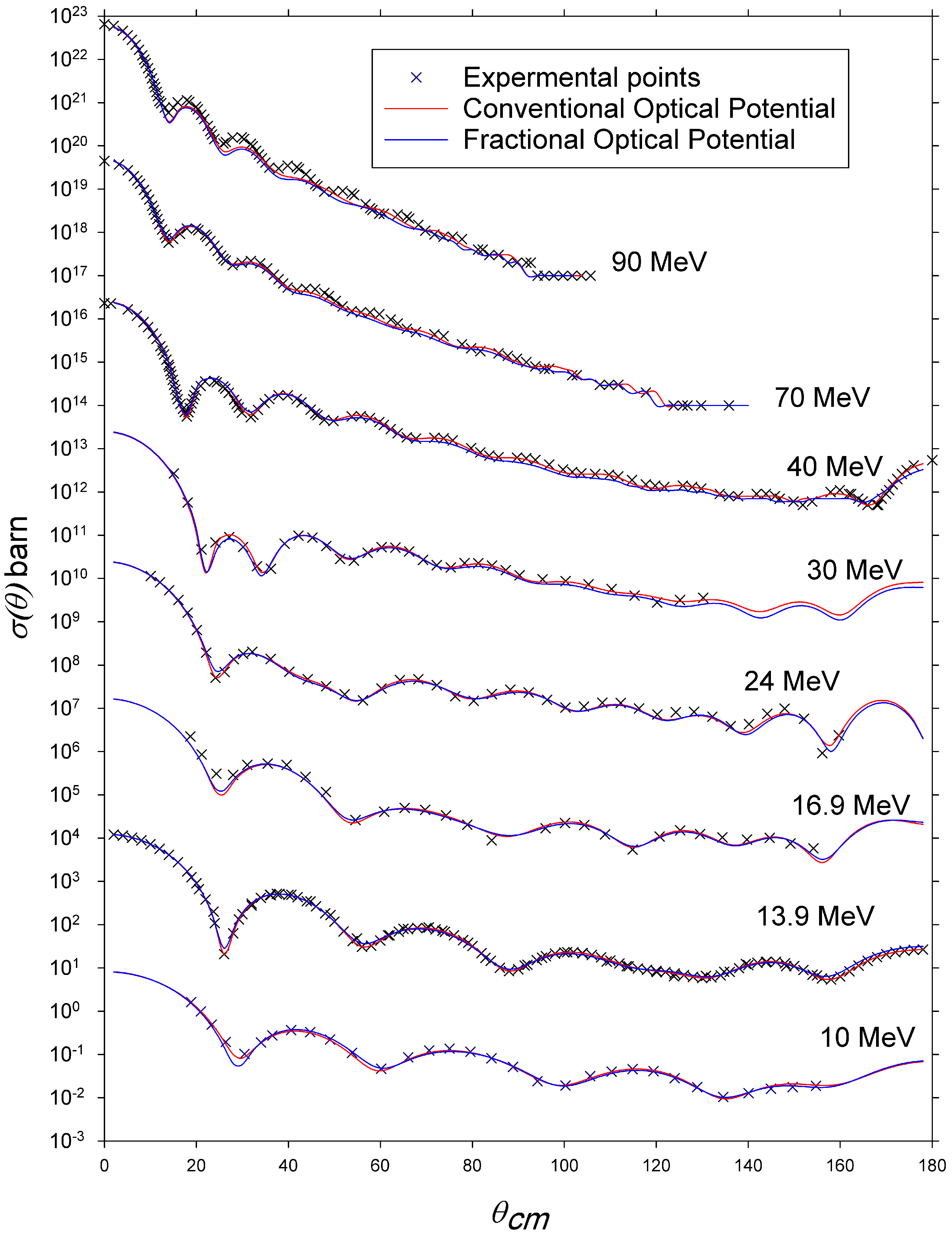
The results of fitting to the experimental data for both conventional optical potentials are shown in Figure 2. It is clear from the figure that there are no noticeable differences between the two potentials, and this is reinforced by the values of ${\chi }^2$ in Table 2 and Table 3.

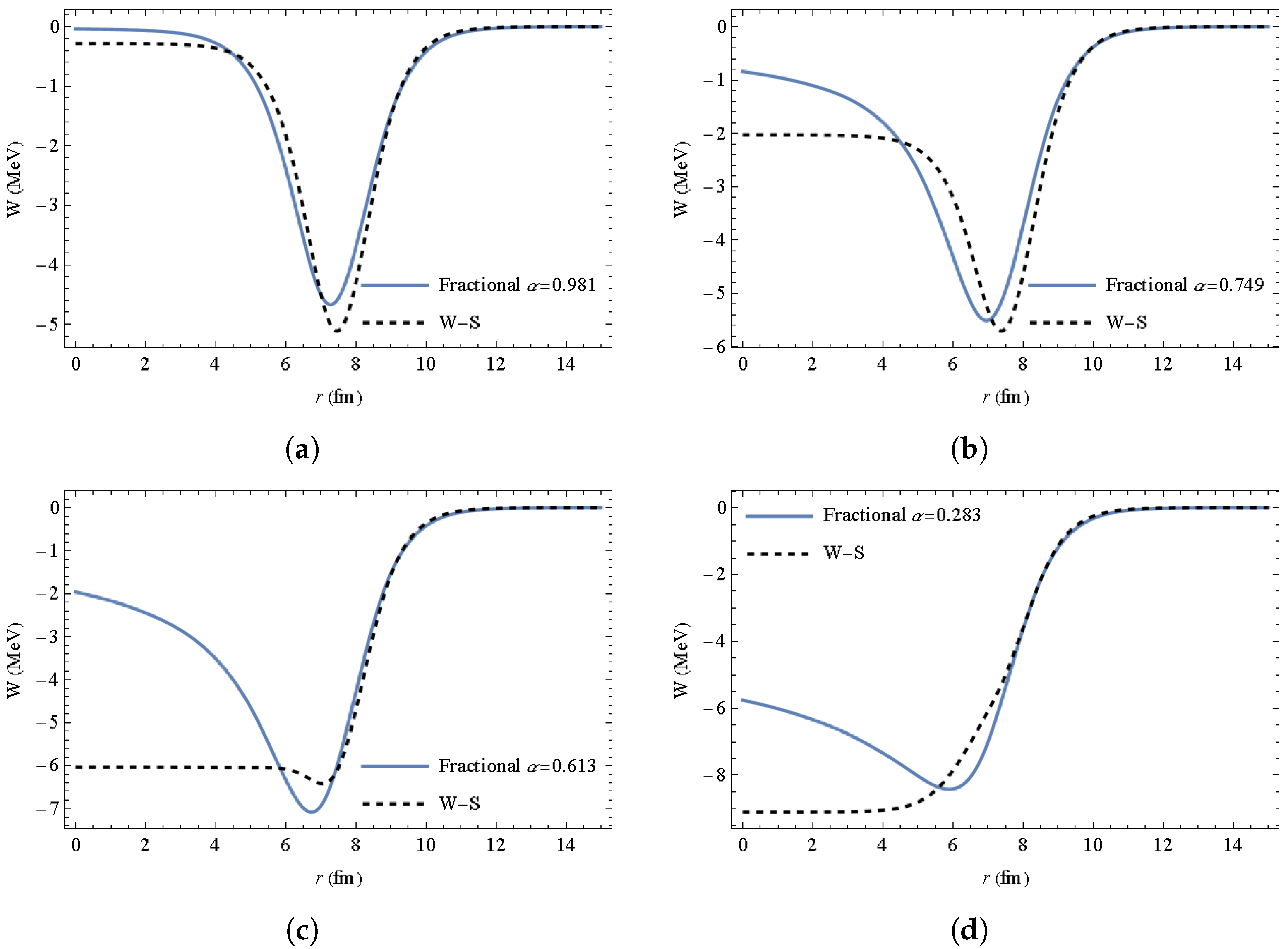
On the other hand, a plot of the absorption term in the optical potential calculated by the Woods–Saxon and its derivative and that calculated by the fractional derivative of the Woods–Saxon at different incident energies are shown in Figure 3. From the figure, one can conclude the following. The two potentials seem to be the same for large r (say, $r>8.5$ fm), which is at the the surface of the target nuclei. As we go deep into the nuclei, the difference is observed between the two potentials; this difference becomes more significant as the incident energy is increased and the volume term of the Woods–Saxon potential becomes dominant. Although the difference is clear between the two models in the inner region of the nucleus, this did not significantly affect the calculation of the differential cross section $\sigma \left(\theta \right)$, which is clearly evident from the values of ${\chi }^2$. This is clear evidence that most of the absorption takes place near the surface and away from the inner region of the nucleus.

However, it is well-known that due to the ambiguity associated with the real and imaginary parts of the optical potential, it is difficult to strictly define the optical potential parameters. A more convenient way to study the behavior of the optical potential is with volume integrals, which are relatively independent of the geometric parameters of the optical potential and give insight on the behavior of the optical potentials, such as the functions of mass, energy, and nuclear asymmetry [16].

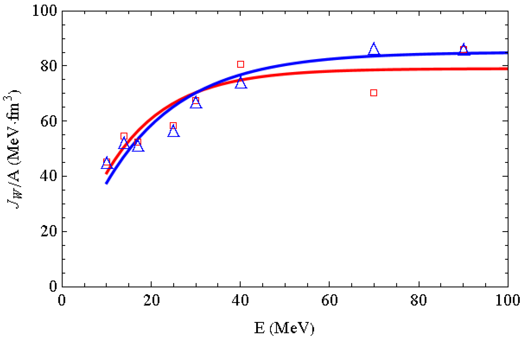
The volume integrals per nucleon of the absorption part of the optical potential are given by

$$J_W/A=\frac{4\pi }{A}{\int }_0^{\infty }{r}^{2}W\left(r\right)dr.$$

(26)

A comparison between the energy dependence of $J_W/A$ obtained by using Woods–Saxon and its derivative as the absorption term and that obtained using the fractional derivative of the Woods–Saxon is shown in Figure 4. Although the two absorption terms are different in the inner region of the nucleus, the volume integrals are almost the same. Again, this indicates that this difference in the inner region of the nucleus has no significant effect on absorption.

Figure 2. (Color online) Elastic neutron scattering from ²⁰⁸Pb. Incident neutron laboratory energies are indicated at the respective angular distributions. The distributions at the bottom represent true cross-section values, while the others are multiplied by factors of ${10}^3,{10}^6$, …Data from [17,18].

Figure 3. (Color online) Absorption term in the optical potential using Woods–Saxon form factor and its derivative (black dashed line) and using the fractional derivative of Woods–Saxon form (blue solid line): (a) 10 MeV, $\alpha =0.981$, (b) 24 MeV, $\alpha =0.749$, (c) 40 MeV, $\alpha =0.613$, (d) 90 MeV, $\alpha =283$.

Figure 4. (Color online) Comparison between the energy dependence of $J_W/A$ obtained by using Woods–Saxon and its derivative (red squares) as the absorption term and that obtained by using the fractional derivative of Woods–Saxon (blue triangles). The solid lines are drawn to guide the eye.

5. Conclusions

In this study, the fractional derivative of the Woods–Saxon form factor as an absorption term in the optical model was examined and compared to the traditional one, which is a Woods–Saxon form and its derivative. As the fractional derivative order $\alpha$ of the Woods–Saxon form factor changes from (1) to (0), its shape transforms from a purely surface to a purely volume one. For values of $0<\alpha <1$, it represents a mixture of surface and volume absorption, which was achieved by adding the volume and absorption terms to the conventional optical potential.