Article

Excitation Functions of Related Temperatures of η and η0 Emission Sources from Squared Momentum Transfer Spectra in High-Energy Collisions

1
Shanxi Institute of Energy, College of Basic Courses, Jinzhong 030600, China
2
State Key Laboratory of Quantum Optics and Quantum Optics Devices, Institute of Theoretical Physics, Shanxi University, Taiyuan 030006, China
3
Collaborative Innovation Center of Extreme Optics, Shanxi University, Taiyuan 030006, China
4
Physical-Technical Institute of Uzbekistan Academy of Sciences, Chingiz Aytmatov str. 2b, Tashkent 100084, Uzbekistan
5
Department of Natural Sciences, National University of Science and Technology MISIS (NUST MISIS), Almalyk Branch, Almalyk 110105, Uzbekistan
*
Authors to whom correspondence should be addressed.
Universe 2023, 9(7), 342; https://doi.org/10.3390/universe9070342
Submission received: 21 June 2023 / Revised: 6 July 2023 / Accepted: 21 July 2023 / Published: 23 July 2023
(This article belongs to the Special Issue Collectivity in High-Energy Proton-Proton and Heavy-Ion Collisions)

Abstract

:
The squared momentum transfer spectra of η and η 0 , produced in high-energy photon–proton ( γ p ) η ( η 0 ) + p processes in electron–proton ( e p ) collisions performed at CEBAF, NINA, CEA, SLAC, DESY, and WLS are analyzed. The Monte Carlo calculations are used in the analysis of the squared momentum transfer spectra, where the transfer undergoes from the incident γ to emitted η ( η 0 ) or equivalently from the target proton to emitted proton. In the calculations, the Erlang distribution and Tsallis–Levy function are used to describe the transverse momentum ( p T ) spectra of emitted particles. Our results show that the average transverse momentum ( p T ), the initial-state temperature ( T i ), and the final-state temperature ( T 0 ) roughly decrease from the lower center-of-mass energy (W) to the higher one in the concerned energy range of a few GeV, which is different from the excitation function from heavy-ion collisions in the similar energy range.

1. Introduction

Abundant experimental data produced at the Large Hadron Collider (LHC) and Relativistic Heavy Ion Collider (RHIC) are helpful for scientists to study the production of Quark–Gluon Plasma (QGP) and the evolution of the collision system. In the process of high-energy heavy-ion collisions, the time evolution of the collision system roughly consists of five stages, which are flight of incoming nuclei, beginning of collisions, strongly-coupled QGP (sQGP), mixed phase, and hadron gas, respectively [1]. In each stage, the evolution picture and property of the collision system, and the distribution law and property of the produced particles, are possibly different from others, because some particles are produced in the earlier processes and others are produced in the last stage.
In the initial stages, two nuclei with the shape of pancake due to the Lorentz contraction move toward each other and collide violently. Because of the transformation from the kinetic energy of the particles to the huge amount of the thermal energy of the system, after a short period of time (∼1 fm/c), QGP is produced which is the extremely hot and dense matter [2,3,4,5]. In the stages of mixed phase and hadron gas, due to the inflation and cooling down of the system, the hadron matter evolves until only color-neutral states are created. In high-energy collisions, the excitation and equilibrium degrees of the system are considered as the important characteristics that can help us to study the mechanism of the nuclear reaction and the characteristics of the system evolution [6,7,8,9,10,11,12,13,14,15].
In the whole process of high-energy collisions, one can use different temperatures to describe the excitation degree of the system or emission source at different stages [16,17,18,19,20,21,22,23]. At the first place, one can choose the initial-state temperature ( T i ) to describe the excitation degree of the system at the beginning of collisions. At the second place, one can use the critical temperature ( T c ) and the chemical freeze-out temperature ( T c h ) to describe the excitation degree of the system in which the hadron matter appears and chemical freeze-out happens separately. At the last place, one can use the kinetic freeze-out or final-state temperature ( T k i n or T 0 ) and the effective temperature ( T e f f ) to describe the excitation degree of the system at the kinetic freeze-out. Here, T e f f includes in addition the flow effect and can be compared with T k i n or T 0 .
As a useful tool for describing the excitation degree of the system, T i represents the temperature of the system or emission source at the initial-stage of collisions [24,25]. This initial-stage refers to a very short stage after the thermalization at the beginning of collisions. To obtain T i , we have several methods. The first method is to solve the state equation of QGP with the fluid model [19]. The second one is to solve the equation for isentropic expansion in relativistic fluid mechanics [16]. The last one is to use the transverse momentum ( p T ) spectra directly, or use various distributions or functions to fit the p T spectra. The last method has special advantages of accuracy and efficiency. This is because there is no need to study the concrete evolution process from QGP or sQGP to hadron phase, but analyze the p T spectra themselves. Usually, we can use the Erlang distribution [26,27,28], Hagedorn function [29], and Tsallis–Levy function [30] for fitting the p T spectra to obtain T i , but in this paper, only the Erlang distribution is selected due to it being the origin of multiple sources in the multi-source thermal model [26,27,28].
The final-state temperature T 0 , known as the kinetic freeze-out temperature, represents the temperature of the system or emission source at the kinetic freeze-out stage. At this stage, the interactions between various particles are negligible, and there are no further elastic collisions in the system. T 0 can be extracted by using the certain distribution or function in fitting the p T spectra, and used to describe the excitation degree of the system. T e f f is similar to T 0 , but there is no influence of flow effect in T 0 . In our previous work [24,25], we have used the Tsallis–Levy function [30] in fitting the p T spectra to estimate T as T e f f . In some small systems such as γ p and γ * p collisions, we have T 0 T , because the flow effect are negligible. In the γ p collisions discussed in this work, we use the Tsallis–Levy function [30] in fitting the p T spectra to extract T ( T e f f ) as T 0 and study the characteristics of the system at the last stage. As for the other temperature types, we do not discuss them in our work anymore.
One can use some parameters to describe the equilibrium degree of the system. By fitting the p T spectra with the Tsallis distribution [31,32], the entropy index q is extracted. Generally, if q is closer to 1, the system is closer to equilibrium, or the equilibrium degree of the system is higher. In the absence of the Tsallis distribution [31,32], one can use the Hagedorn function [29] or Tsallis–Levy function [30] alternatively. In the fitting process, q can be abstracted by introducing n, which is used to describe the equilibrium degree of the system indirectly due to n = 1 / ( q 1 ) . In this work, let n be fixed, then we may obtain T i and T 0 more conveniently to describe the excitation degree of the system. It should be noted that when considering the equilibrium issue, small systems are also possible because we consider a large number of events within the framework of giant canonical ensemble.
To obtain the above-mentioned temperatures and p T , we need to use the p T spectra. In the absence of the p T spectra, we can use the squared momentum transfer ( | t | ) spectra alternatively. The squared momentum transfer is one of the Mandelstam variables which consists of the four-momentum of the concerned particles [33]. In the fitting process, the squared momentum transfer spectra cannot be fitted by those distributions and functions directly. Instead, we can obtain many concrete p T satisfying certain distribution, then we can obtain many concrete values of the squared momentum transfer with the Monte Carlo calculation. Finally, we can obtain the distribution of the squared momentum transfer.
In this paper, the squared momentum transfer spectra of η and η 0 , produced in high-energy γ p collisions performed at the Continuous Electron Beam Accelerator Facility (CEBAF) [34], the Daresbury Laboratory electron synchrotron NINA [35], the Cambridge Electron Accelerator (CEA) [36], the Stanford Linear Accelerator Center (SLAC) [37], the Deutsches Elektronen-Synchrotron (DESY) [38], and the Wilson Laboratory Synchrotron (WLS) [39] are fitted by the results obtained with the Monte Carlo method. These experimental data are measured at different center-of-mass energies (W) and incident photon energies ( E γ ).
The remainder of this article is structured as follows. The formalism and method are described in Section 2. Results and discussion are given in Section 3. In Section 4, we give our summary and conclusions.

2. Picture and Formalism

2.1. The Erlang Distribution

The Erlang distribution, which describes the p T spectra and multiplicity distribution, can be obtained from the multi-source thermal model [26,27,28], where the multiplicity is defined as the number of particles produced in an event. The model assumes that multiple sources are formed and contribute to p T of the considered particles in the collision process. These sources are considered as nucleons or partons if we study the formation of nucleon clusters (nuclear fragments) or particles. Generally speaking, it is enough to use one- or two-component Erlang distribution in fitting the p T spectra.
The Erlang distribution is the convolution of multiple exponential distributions [26,27,28]. Every exponential distribution represents the transverse momentum ( p t ) distribution obeyed by a parton, and can be regarded as
f ( p t j ) = 1 p t exp p t j p t .
Here, j, p t j , and p t refer to the index of participant partons, the transverse momentum which depends on j, and the average contribution of participant partons to p T of the considered particles, respectively.
It is assumed that n s partons contribute to p T of a given particle. We have the Erlang p T distribution to be
f 1 ( p T ) = 1 N d N d p T = p T n s 1 ( n s 1 ) ! p t n s exp p T p t .
In Equation (2), the p T of a given particle consists of p t 1 , p t 2 , …, p t n s of n s partons. Here, n s is not large and it is around 2–5. This is because n s is not determined by the collision system, but by the number of partons contributing to a given p T . As for N, it is the number of particles, and it depends on the collision system. It is natural that 0 f 1 ( p T ) d p T = 1 because f 1 ( p T ) is a probability density function.

2.2. The Tsallis–Levy Function

The Tsallis–Levy function is one of the applications of the Tsallis statistics [31] in high-energy collisions. We have p T distribution in form of the Tsallis–Levy function [30] to be
f 2 ( p T ) = 1 N d N d p T = C p T 1 + p T 2 + m 0 2 m 0 n T ( n + 1 ) .
Here, T and n are free parameters, p T 2 + m 0 2 = m T is the transverse mass, m 0 is the rest mass of the considered particle, and C is the normalization constant, which is related to T, n, and m 0 to make 0 f 2 ( p T ) d p T = 1 . Due to particle mass m 0 appearing in p T 2 + m 0 2 m 0 in Equation (3), f 2 ( p T ) is related to m 0 . Our tentative calculation shows that m 0 mainly affects the normalization and weakly the tendency of the function.
In the fitting process of the p T spectra with the Tsallis–Levy function [30], we can obtain T, which is used to describe the excitation degree of system at the kinetic freeze-out stage. The influence of flow effect is included in T compared with T 0 . In general, T > T 0 , but in the γ p collision discussed in this work, due to the flow effect being small and considered negligible, we are of the opinion that T T 0 roughly. To obtain the excitation function of T more conveniently, we set n as a fixed value in the fitting with the Tsallis–Levy function [30].

2.3. Average Transverse Momentum and Initial-State Temperature

In the process of fitting p T spectra with the Erlang distribution [26,27,28], p T and T i are estimated and used to describe the excitation degree of the system. In fact, p T can be obtained by
p T = 0 p T f 1 ( p T ) d p T = n s p t .
To obtain T i , we need to use a color string percolation method [40,41,42], which gives
T i = p T 2 2 F ( ξ ) ,
where
p T 2 = 0 p T 2 f 1 ( p T ) d p T = n s ( n s + 1 ) p t 2
and F ( ξ ) is the color suppression factor. Although f 2 ( p T ) can be also used in the calculation of p T and p T 2 , it is more convenient to use f 1 ( p T ) from which specific results for p T and p T 2 can be obtained from the integration.
It is necessary to discuss the application of color string percolation method. In the process of using this method, we can determine the number of strings used. For instance, only one string is used in present work, that is to say F ( ξ ) = 1 [43]. If we consider other strings, there will be the minimum F ( ξ ) 0.6 , which results in the maximum increase of 29.1% in T i [43]. Although it is possible to have any other strings in this work, they do not have a great influence on T i . This is because one string accounts for a large proportion, but two and multiple strings account for a small one.

2.4. The Squared Momentum Transfer

In the center-of-mass reference frame, in two-body reaction 2 + 1 4 + 3 or two-body-like reaction, three Mandelstam variables [33], s, t, and u are defined. They are composed of four-momenta of participated particles, and their forms are
s = ( P 1 + P 2 ) 2 = ( P 3 + P 4 ) 2 ,
t = ( P 1 P 3 ) 2 = ( P 2 + P 4 ) 2 ,
and
u = ( P 1 P 4 ) 2 = ( P 2 + P 3 ) 2 ,
respectively. Here, P 1 , P 2 , P 3 , and P 4 are four-momenta of particles 1, 2, 3, and 4, separately. Particle 1 is the target proton, which is supposed to be incident along the O z direction, and particle 2 is the incident γ , which is supposed to be incident along the opposite direction. After the collisions, particle 3 is the emitted proton, which is emitted with angle θ relative to the O z direction, and particle 4 is the emitted meson, which is emitted along the opposite direction.
Due to different forms of Mandelstam variables, the physical meanings of s, t, and u are different. s is supposed to be the center-of-mass energy, both u and t refer to the squared momentum transfer between particles. In this work, we choose variable t to research, and its form is
| t | = | ( E 1 E 3 ) 2 ( p 1 p 3 ) 2 | = m 1 2 + m 3 2 2 E 1 p 3 T sin θ 2 + m 3 2 + 2 E 1 2 m 1 2 p 3 T tan θ ,
where E 1 and E 3 , p 1 and p 3 , as well as m 1 and m 3 are the energy, momentum, and rest mass of particles 1 and 3, respectively. Besides, p 3 T is the transverse momentum of particle 3, which obeys Equation (2) or (3).
In this paper, we select the squared momentum transfer spectra at different center-of-mass energy W and incident photon energy E γ to analyze. The center-of-mass energy is W = s = ( P 1 + P 2 ) 2 in our analysis [24,25]. Let Q 2 and x B be the squared photon virtuality and Bjorken scaling variable, and we have W 2 Q 2 / x B [44,45,46,47,48,49,50,51].

2.5. The Process of Monte Carlo Calculations

Although we can use Equation (10) to obtain the single squared momentum transfer, its distribution is difficult to obtain. To obtain the squared momentum transfer distribution, we can execute the following steps. First, we produce many concrete p 3 T satisfied with Equation (2) or (3) and θ . Second, we can obtain many concrete squared momentum transfer by calculating with Equation (10) repeatedly. Lastly, the squared momentum transfer distribution is obtained with the statistical method.
To produce many concrete p 3 T and θ , we may use the Monte Carlo method. Let R 1 , 2 and r 1 , 2 , 3 , , n s be random numbers distributed evenly in [ 0 , 1 ] . Then, we obtain many concrete p 3 T by solving this equation:
0 p T f p T d p T < R 1 < 0 p T + δ p T f p T d p T ,
where δ p T is a small shift relative to p T , and f ( p T ) represents Equation (2) or (3). As for Equation (2), there is a simpler expression of p T . We can solve the equation
0 p t j f p t j d p t j = r j ( j = 1 , 2 , 3 , , n s ) ,
which results in
p t j = p t ln r j ( j = 1 , 2 , 3 , , n s ) .
In this way, the simpler expression is written as
p T = j = 1 n s p t j = p t j = 1 n s ln r j = p t ln j = 1 n s r j .
The distribution of θ satisfies with
f θ θ = 1 2 sin θ
which is the half-sine function. In the source’s rest frame, it is obtained under the assumption of isotropic emission. Solving the equation
0 θ f θ θ d θ = R 2 ,
we have
θ = 2 arcsin R 2
which is used in our calculations.
The squared momentum transfer distribution obtained using the above steps is used to fit the experimental data measured at different W and E γ . In the fitting process, parameters p t , n s , T are extracted with the method of least squares, and n is fixed to be large enough for convenience. Then, we can obtain p T from Equation (4) and T i from Equation (5). The errors of parameters are obtained by the general method of statistical simulation.

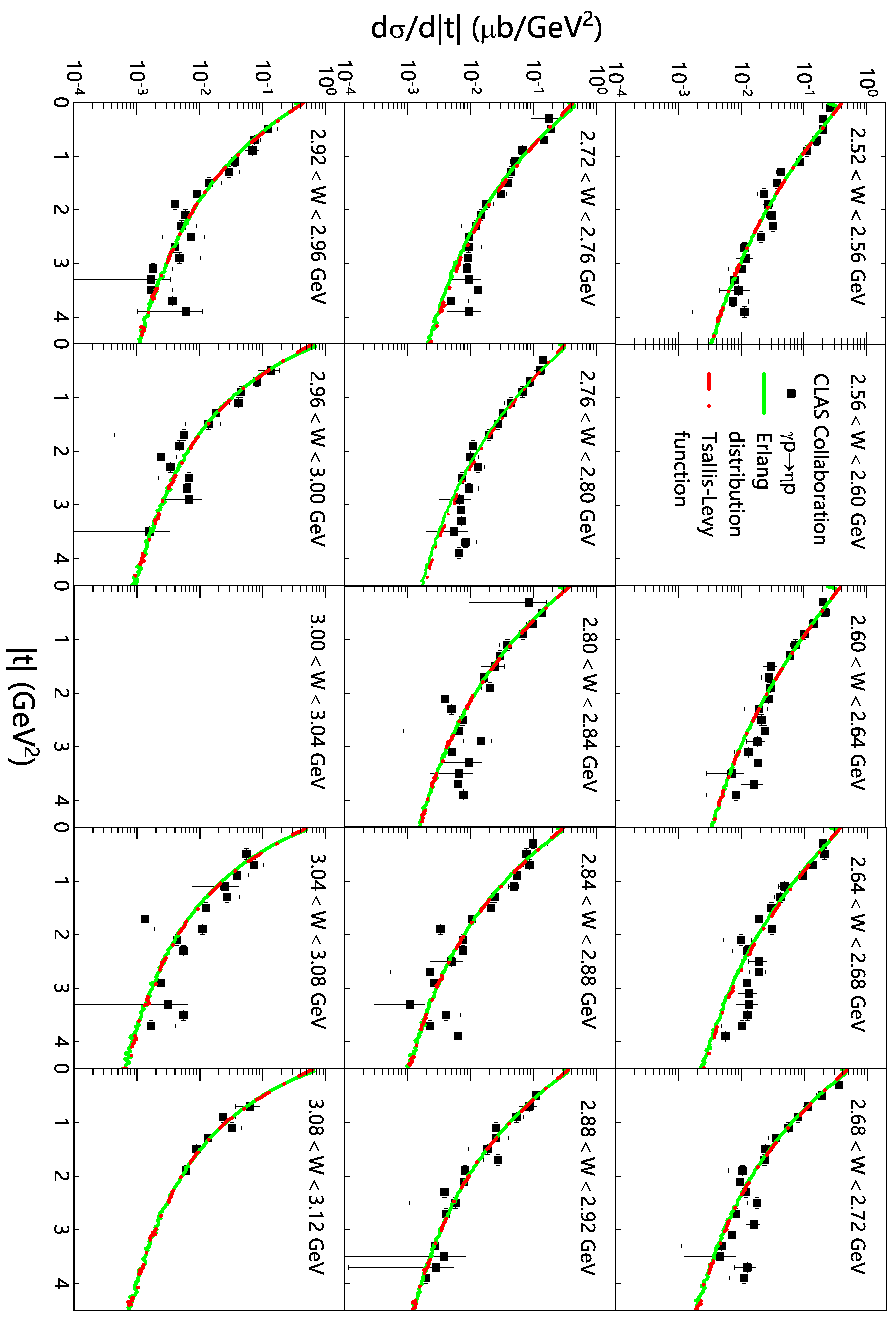
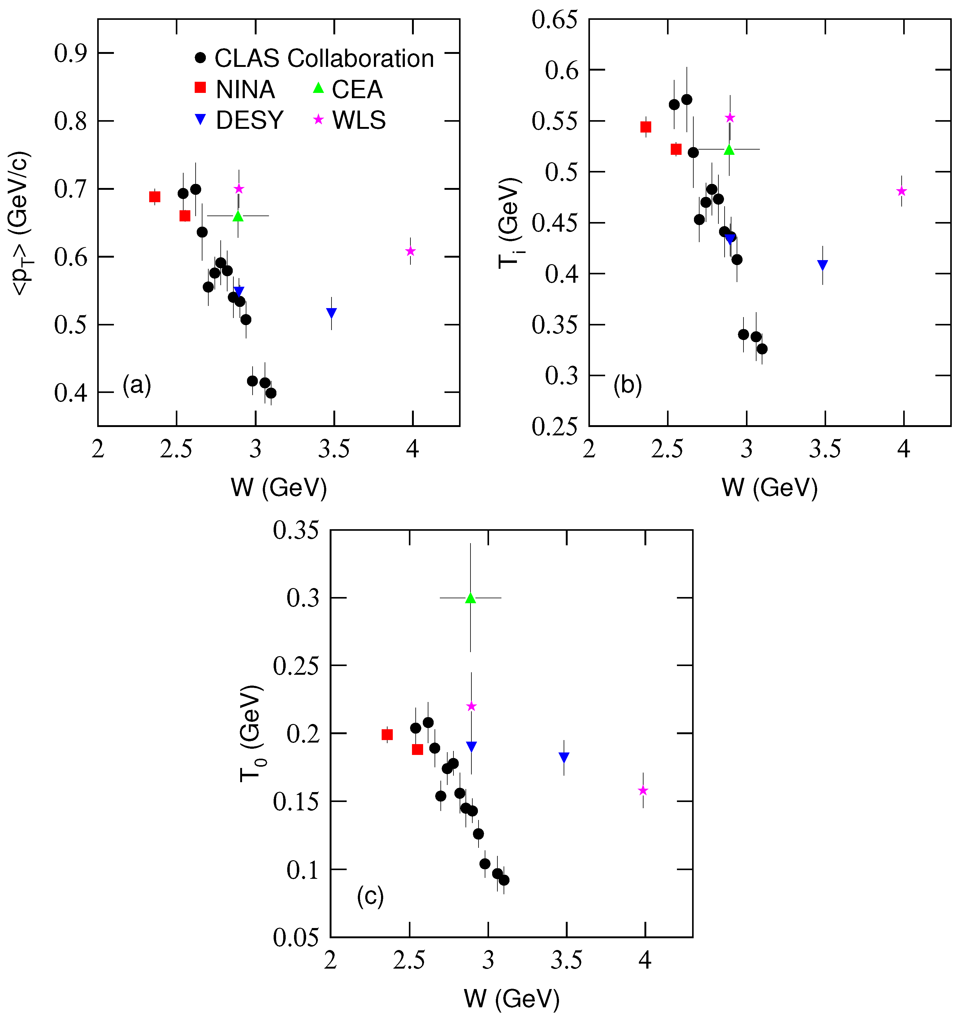
3. Results and Discussion

Figure 1 shows the differential cross-section, d σ / d | t | , in the squared momentum transfer | t | of γ p η p produced in different center-of-mass energy ranges 2.52 < W < 2.56 , 2.60 < W < 2.64 , 2.64 < W < 2.68 , 2.68 < W < 2.72 , 2.72 < W < 2.76 , 2.76 < W < 2.80 , 2.80 < W < 2.84 , 2.84 < W < 2.88 , 2.88 < W < 2.92 , 2.92 < W < 2.96 , 2.96 < W < 3.00 , 3.04 < W < 3.08 , and 3.08 < W < 3.12 GeV, corresponding to the incident photon energy range E γ 2.91 , 4.72 GeV. The black squares represent the experimental data performed at the CEBAF and measured by the CEBAF Large Acceptance Spectrometer (CLAS) Collaboration [34], where the data in 2.56 < W < 2.60 and 3.00 < W < 3.04 GeV are not available from the experiment. The green solid curves and red-dash-dotted curves are the statistical results of | t | , in which p T satisfies the Erlang distribution and Tsallis–Levy function, respectively. One can see that the fitting results are in agreement with the experimental data.
In the fitting process, the average transverse momentum p t contributed by participant partons, the number n s of participant partons, and the effective temperature T of the emission source are extracted. With the values of p t and n s , the average transverse momentum p T of final-state particles and the initial-state temperature T i of the emission source are obtained naturally. To obtain T 0 more conveniently, we take n = 40 ( q = 1.025 ) in the Tsallis–Levy function [30]. Here, T 0 T in the function for the small system γ p or e p process in which the effect of collective flow is neglected. In addition, E 1 = 0.938 GeV in Equation (10). In Table 1, we list the values of free parameters p t and n s , derived parameter T i , and χ 2 /ndof for the fit of Erlang distribution, as well as the values of free parameter T and χ 2 /ndof for the fit of Tsallis–Levy function.
Similar to Figure 1, Figure 2 presents the differential cross-section, d σ / d | t | , in | t | of (a, d, e) γ p η p and (b, c) γ p η 0 p produced at (a) NINA [35], (b) CEA [36], (c) SLAC [37], (d) DESY [38], and (e) WLS [39] at (a) W = 2.36, 2.551 GeV, in (b) 2.694 GeV < W < 3.084 GeV, at (c) E γ = 6 GeV, (d) W = 2.895, 3.484 GeV, and (e) W = 2.895, 3.986 GeV. The symbols in Figure 2 represent the experimental data. The black solid and dashed curves are the statistical results of | t | in which p T satisfies the Erlang distribution and Tsallis–Levy function, respectively. The values of the parameters and χ 2 /ndof are listed in Table 1. One can see that the statistical results are in approximate agreement with the experimental data.
The dependences of (a) p T , (b) T i , and (c) T 0 on center-of-mass energy (W) are given in Figure 3. The different symbols represent the parameter values extracted from Figure 1 and Figure 2. For the results from the CLAS Collaboration, one can see that p T , T i , and T 0 decrease generally with an increase in W. For the results from the other cases, the trends are not clear. In the fitting process of experimental data produced at CEA and DESY, we consider that the ranges of | t | are wider than others. To fit better, there is a big difference between the statistical results of | t | in which p T satisfies the Erlang distribution and Tsallis–Levy function, and it results in a higher T 0 extracted from the statistical results of | t | , in which p T satisfies the Tsallis–Levy function.
From Figure 3, it should be noted that the results for CEA and WLS overlap for p T and T i , but differ significantly for T 0 , at W 3 GeV. The reason is that both p T and T i are from the Erlang distribution and T 0 is from the Tsallis–Levy function. In most cases, the two fits are similar to each other. In a few cases (Figure 2b,d), the two fits (the solid and dashed curves) are inharmonious. If we try to obtain a similar result for the two fits in a given range of | t | (e.g., | t | > 0.2 GeV 2 ), a few data (the first or second one) will deviate greatly from the fit. That is, we may adjust the parameters in Figure 3c to be harmonious. However, a worse fit will be obtained. Due to the two inharmonious fits in Figure 2b, if the two fits of the Erlang distribution in Figure 2b,e are harmonious (Figure 3a,b), the two fits of the Tsallis–Levy function in the two panels are inharmonious (Figure 3c). In addition, because two parameters are used in the Erlang distribution and one parameter is used in the Tsallis–Levy function, the former is more flexible than the latter in the fit.
Generally speaking, p T , T i , and T 0 increase with the increase of W in heavy-ion collisions at a few GeV energy [10,17,18,19,20,21,23,43], which is the energy range discussed in this work. Compared with heavy-ion collisions, in γ p η p reaction the situation is different due to the absence of a secondary collision process and a cold nuclear effect in the small system. In addition, the small system does not have enough time to react at higher energies. This implies that the small system has a lower excitation degree at higher energies. Although this work confirms our previous work [24], the energy range discussed by us is narrow, and the data cited here are measured at different devices with low statistics and large errors in most cases. To obtain more solid and explicit conclusions regarding the evolution of the parameters with changing the energy, significantly higher statistics of the experimental data are required in the future.
Before the summary and conclusions, we would like to point out that although the multiplicity is only two in the two-body reaction discussed in the present work, we have used the parametrization from the Erlang distribution and Tsallis–Levy function due to lots of events being collected in experiments. This case can be compared with the grand canonical ensemble in statistical physics. Although the particles in different events do not have interactions and the multiplicity in each event is very low, these particles have the same or similar production conditions due to the same or similar events with given collision energies. Therefore, we think that the particles in many events obey some statistical laws. In addition, as a reflection of the average kinetic energy of the thermal or disorganized motion, the concept of temperature is applicable in the field of high energy collisions, even two-body reaction.

4. Summary and Conclusions

The squared momentum transfer spectra of η and η 0 produced in the two-body process γ p η ( η 0 ) + p have been analyzed by the statistical results of | t | , in which p T satisfies the Erlang distribution and Tsallis–Levy function, respectively. The squared momentum transfer undergoes from the incident γ to emitted η or η 0 , or also equivalently from the target proton to the emitted proton. The statistical results are in agreement with the experimental data measured at different experiments. In the fitting process, free parameters p t , n s , and T are extracted. Then, we obtain the dependencies of p T , T i , and T 0 on center-of-mass energy W.
At a few GeV, it is believed that p T , T i , and T 0 increase generally with an increase in W in heavy-ion collisions. However, in γ p η p reaction, the situation is different due to the absence of a secondary collision process and cold nuclear effect in the small system. Meanwhile, the small system has not enough time to react at higher energy. This implies that the small system has a lower excitation degree at higher energy. The excitation functions of the concerned parameters in the large and small systems have different tendencies. More data are required in the future to compare the excitation functions in the two kinds of systems.

Author Contributions

The authors contributed to the paper in this way: conceptualization, F.-H.L. and K.K.O.; methodology, F.-H.L. and K.K.O.; software, Q.W.; validation, F.-H.L. and K.K.O.; formal analysis, Q.W.; investigation, Q.W.; resources, Q.W.; data curation, Q.W.; writing—original draft preparation, Q.W.; writing—review and editing, F.-H.L. and K.K.O.; visualization, Q.W.; supervision, F.-H.L. and K.K.O.; project administration, Q.W. and F.-H.L.; funding acquisition, Q.W., F.-H.L. and K.K.O. All authors have read and agreed to the published version of the manuscript.

Funding

The work of Q.W. was supported by the Shanxi Provincial Natural Science Foundation under Grant No. 2023 and the Doctoral Scientific Research Foundations of Shanxi Province and Shanxi Institute of Energy. The work of F.-H.L. was supported by the National Natural Science Foundation of China under Grant No. 12147215, the Shanxi Provincial Natural Science Foundation under Grant No. 202103021224036, and the Fund for Shanxi “1331 Project” Key Subjects Construction. The work of K.K.O. was supported by the Ministry of Innovative Development of the Republic of Uzbekistan within the fundamental project No. F3-20200929146 on analysis of open data on heavy-ion collisions at RHIC and LHC.

Data Availability Statement

The data used to support the findings of this study are included within the article and are cited at relevant places within the text as references.

Conflicts of Interest

The authors declare that there are no conflicts of interest regarding the publication of this paper. The funders had no role in the design of the study; in the collection, analysis, or interpretation of the data; in the writing of the manuscript; or in the decision to publish the results.

References

  1. Caines, H. What’s interesting about strangeness production? An overview of recent results. J. Phys. G 2005, 31, S101–S117. [Google Scholar] [CrossRef] [Green Version]
  2. Shuryak, E.V. Quantum chromodynamics and the theory of superdense matter. Phys. Rep. 1980, 61, 71–158. [Google Scholar] [CrossRef]
  3. Digal, S.; Petreczky, P.; Satz, H. Quarkonium feed-down and sequential suppression. Phys. Rev. D 2001, 64, 094015. [Google Scholar] [CrossRef] [Green Version]
  4. Karsch, F.; Kharzeev, D.; Satz, H. Sequential charmonium dissociation. Phys. Lett. B 2006, 637, 75–80. [Google Scholar] [CrossRef] [Green Version]
  5. Braun-Munzinger, P.; Stachel, J. The quest for the quark-gluon plasma. Nature 2007, 448, 302–309. [Google Scholar] [CrossRef]
  6. Wang, H.; Chen, J.-H.; Ma, Y.-G.; Zhang, S. Charm hadron azimuthal angular correlations in Au+Au collisions at s N N = 200 GeV from parton scatterings. Nucl. Sci. Tech. 2019, 30, 185. [Google Scholar] [CrossRef]
  7. Yan, T.-Z.; Li, S.; Wang, Y.-N.; Xie, F.; Yan, T.-F. Yield ratios and directed flows of light particles from proton-rich nuclei-induced collisions. Nucl. Sci. Tech. 2019, 30, 15. [Google Scholar] [CrossRef]
  8. Fisli, M.; Mebarki, N. Top quark pair-production in noncommutative standard model. Adv. High Energy Phys. 2020, 2020, 7279627. [Google Scholar] [CrossRef]
  9. He, X.-W.; Wu, F.-M.; Wei, H.-R.; Hong, B.-H. Energy-dependent chemical potentials of light hadrons and quarks based on transverse momentum spectra and yield ratios of negative to positive particles. Adv. High Energy Phys. 2020, 2020, 1265090. [Google Scholar] [CrossRef]
  10. Waqas, M.; Li, B.-C. Kinetic freeze-out temperature and transverse flow velocity in Au-Au collisions at RHIC-BES energies. Adv. High Energy Phys. 2020, 2020, 1787183. [Google Scholar] [CrossRef] [Green Version]
  11. Tang, Z.-B.; Zha, W.-M.; Zhang, Y.-F. An experimental review of open heavy flavor and quarkonium production at RHIC. Nucl. Sci. Tech. 2020, 31, 81. [Google Scholar] [CrossRef]
  12. Shen, C.; Yan, L. Recent development of hydrodynamic modeling in heavy-ion collisions. Nucl. Sci. Tech. 2020, 31, 122. [Google Scholar] [CrossRef]
  13. Yu, H.; Fang, D.-Q.; Ma, Y.-G. Investigation of the symmetry energy of nuclear matter using isospin-dependent quantum molecular dynamics. Nucl. Sci. Tech. 2020, 31, 61. [Google Scholar] [CrossRef]
  14. Bhaduri, S.; Bhaduri, A.; Ghosh, D. Study of di-muon production process in pp collision in CMS data from symmetry scaling perspective. Adv. High Energy Phys. 2020, 2020, 4510897. [Google Scholar] [CrossRef] [Green Version]
  15. Tawfik, A.N. Out-of-equilibrium transverse momentum spectra of pions at LHC energies. Adv. High Energy Phys. 2019, 2019, 4604608. [Google Scholar] [CrossRef]
  16. Nayak, J.K.; Alam, J.; Sarkar, S.; Sinha, B. Measuring initial temperature through a photon to dilepton ratio in heavy-ion collisions. J. Phys. G 2008, 35, 104161. [Google Scholar] [CrossRef]
  17. Adare, A. et al. [PHENIX Collaboration] Enhanced production of direct photons in Au+Au collisions at s N N = 200 GeV and implications for the initial temperature. Phys. Rev. Lett. 2010, 104, 132301. [Google Scholar] [CrossRef] [Green Version]
  18. Csanád, M.; Májer, I. Initial temperature and EoS of quark matter via direct photons. Phys. Part. Nuclei Lett. 2011, 8, 1013–1015. [Google Scholar] [CrossRef]
  19. Csanád, M.; Májer, I. Equation of state and initial temperature of quark gluon plasma at RHIC. Cent. Eur. J. Phys. 2012, 10, 850–857. [Google Scholar] [CrossRef] [Green Version]
  20. Soltz, R.A.; Garishvili, I.; Cheng, M.; Abelev, B.; Glenn, A.; Newby, J.; Levy, L.A.L.; Pratt, S. Constraining the initial temperature and shear viscosity in a hybrid hydrodynamic model of s N N = 200 GeV Au+Au collisions using pion spectra, elliptic flow, and femtoscopic radii. Phys. Rev. C 2013, 87, 044901. [Google Scholar] [CrossRef] [Green Version]
  21. Waqas, M.; Liu, F.-H. Initial, effective, and kinetic freeze-out temperatures from transverse momentum spectra in high-energy proton(deuteron)-nucleus and nucleus-nucleus collisions. Eur. Phys. J. Plus 2020, 135, 147. [Google Scholar] [CrossRef]
  22. Cleymans, J.; Paradza, M.W. Tsallis statistics in high energy physics: Chemical and thermal freeze-outs. Physics 2020, 2, 654–664. [Google Scholar] [CrossRef]
  23. Li, L.-L.; Liu, F.-H. Kinetic freeze-out properties from transverse momentum spectra of pions in high energy proton-proton collisions. Physics 2020, 2, 277–308. [Google Scholar] [CrossRef]
  24. Wang, Q.; Liu, F.-H.; Olimov, K.K. Initial- and final-state temperatures of emission source from differential cross-section in squared momentum transfer in high-energy collisions. Adv. High Energy Phys. 2021, 2021, 6677885. [Google Scholar] [CrossRef]
  25. Wang, Q.; Liu, F.-H.; Olimov, K.K. Initial-state temperature of light meson emission source From squared momentum transfer spectra in high-energy collisions. Front. Phys. 2021, 9, 792039. [Google Scholar] [CrossRef]
  26. Liu, F.-H.; Li, J.-S. Isotopic production cross section of fragments in 56Fe+p and 136Xe (124Xe)+Pb reactions over an energy range from 300A to 1500A MeV. Phys. Rev. C 2008, 78, 044602. [Google Scholar] [CrossRef]
  27. Liu, F.-H. Unified description of multiplicity distributions of final-state particles produced in collisions at high energies. Nucl. Phys. A 2008, 810, 159–172. [Google Scholar] [CrossRef]
  28. Liu, F.-H.; Gao, Y.-Q.; Tian, T.; Li, B.-C. Unified description of transverse momentum spectrums contributed by soft and hard processes in high-energy nuclear collisions. Eur. Phys. J. A 2014, 50, 94. [Google Scholar] [CrossRef]
  29. Hagedorn, R. Multiplicities, pT distributions and the expected hadron → quark-gluon phase transition. Riv. Nuovo Cim. 1983, 6, 1–50. [Google Scholar] [CrossRef]
  30. Abelev, B. et al. [ALICE Collaboration] Production of Σ(1385)± and Ξ(1530)0 in proton-proton collisions at s = 7 TeV. Eur. Phys. J. C 2015, 75, 1–19. [Google Scholar]
  31. Tsallis, C. Possible generalization of Boltzmann-Gibbs statistics. J. Stat. Phys. 1988, 52, 479–487. [Google Scholar] [CrossRef]
  32. Abelev, B.I. et al. [STAR Collaboration] Strange particle production in p+p collisions at s = 200 GeV. Phys. Rev. C 2007, 75, 064901. [Google Scholar] [CrossRef] [Green Version]
  33. Zhang, N.-S. Particle Physics (Volume I); Science Press: Beijing, China, 1986. [Google Scholar]
  34. Hu, T. et al. [CLAS Collaboration] Photoproduction of η mesons off the proton for 1.2<Eγ<4.7 GeV using CLAS at Jefferson Laboratory. Phys. Rev. C 2020, 102, 065203. [Google Scholar]
  35. Bussey, P.J.; Raine, C.; Rutherglen, J.G.; Booth, P.S.L.; Carroll, L.J.; Daniel, P.R.; Edwards, A.W.; Hardwick, C.J.; Holt, J.R.; Jackson, J.N. et al. The polarized beam asymmetry in photoproduction of eta mesons from protons at 2.5 GeV and 3.0 GeV. Phys. Lett. B 1976, 61, 479–482. [Google Scholar] [CrossRef]
  36. Bellenger, D.; Deutsch, S.; Luckey, D.; Osborne, L.S.; Schwitters, R. Photoproduction of η0 mesons at 4 GeV. Phys. Rev. Lett. 1968, 21, 1205–1208. [Google Scholar] [CrossRef]
  37. Anderson, R.; Gustavson, D.; Johnson, J.; Ritson, D.; Jones, W.G.; Kreinick, D.; Murphy, F.; Weinstein, R. Measurements of π0 and η0 photoproduction at incident gamma-ray energies of 6.0-17.8 GeV. Phys. Rev. Lett. 1968, 21, 384–386. [Google Scholar] [CrossRef]
  38. Braunschweig, W.; Erlewein, W.; Frese, H.; Lübelsmeyer, K.; Meyer-Wachsmuth, H.; Schmitz, D.; Schultz von Dratzig, A.; Wessels, G. Single photoproduction of η-mesons of hydrogen in the forward direction at 4 and 6 GeV. Phys. Lett. B 1970, 33, 236–240. [Google Scholar] [CrossRef]
  39. Dewire, J.; Gittelman, B.; Loe, R.; Loh, E.C.; Ritchie, D.J.; Lewis, R.A. Photoproduction of eta mesons from hydrogen. Phys. Lett. B 1971, 37, 326–328. [Google Scholar] [CrossRef]
  40. Gutay, L.J.; Hirsch, A.S.; Scharenberg, R.P.; Srivastava, B.K.; Pajares, C. De-confinement in small systems: Clustering of color sources in high multiplicity p¯p collisions at s = 1.8 TeV. Int. J. Mod. Phys. E 2015, 24, 1550101. [Google Scholar] [CrossRef] [Green Version]
  41. Scharenberg, R.P.; Srivastava, B.K.; Pajares, C. Exploring the initial stage of high multiplicity proton-proton collisions by determining the initial temperature of the quark-gluon plasma. Phys. Rev. D 2019, 100, 114040. [Google Scholar] [CrossRef] [Green Version]
  42. Sahoo, P.; De, S.; Tiwari, S.K.; Sahoo, R. Energy and centrality dependent study of deconfinement phase transition in a color string percolation approach at RHIC energies. Eur. Phys. J. A 2018, 54, 136. [Google Scholar] [CrossRef] [Green Version]
  43. Wang, Q.; Liu, F.-H. Excitation function of initial temperature of heavy flavor quarkonium emission source in high energy collisions. Adv. High Energy Phys. 2020, 2020, 5031494. [Google Scholar] [CrossRef]
  44. Aaron, F.D. et al. [H1 Collaboration] Diffractive electroproduction of ρ and ϕ mesons at HERA. J. High Energy Phys. 2010, 2010, 032. [Google Scholar] [CrossRef] [Green Version]
  45. Aktas, A. et al. [H1 Collaboration] Elastic J/ψ production at HERA. Eur. Phys. J. C 2006, 46, 585–603. [Google Scholar] [CrossRef]
  46. Chekanov, S. et al. [ZEUS Collaboration] Exclusive ρ0 production in deep inelastic scattering at HERA. PMC Phys. A 2007, 1, 6. [Google Scholar] [CrossRef] [Green Version]
  47. Derrick, M. et al. [ZEUS Collaboration] Measurement of elastic ω photoproduction at HERA ZEUS Collaboration. Z. Phys. C 1997, 73, 73–84. [Google Scholar]
  48. Chekanov, S. et al. [ZEUS Collaboration] Exclusive electroproduction of ϕ mesons at HERA. Nucl. Phys. B 2005, 718, 3–31. [Google Scholar] [CrossRef] [Green Version]
  49. Chekanov, S. et al. [ZEUS Collaboration] Exclusive electroproduction of J/ψ mesons at HERA. Nucl. Phys. B 2004, 695, 3–37. [Google Scholar] [CrossRef] [Green Version]
  50. Barberis, D. et al. [WA102 Collaboration] A coupled channel analysis of the centrally produced K+K and π+π final states in pp interactions at 450 GeV/c. Phys. Lett. B 1999, 462, 462–470. [Google Scholar] [CrossRef] [Green Version]
  51. Barberis, D. et al. [WA102 Collaboration] A measurement of the branching fractions of the f1(1285) and f1(1420) produced in central pp interactions at 450 GeV/c. Phys. Lett. B 1998, 440, 225–232. [Google Scholar] [CrossRef] [Green Version]
Figure 1. The differential cross-section d σ / d | t | in | t | of γ p η p process produced in e p collisions at energy ranges shown in the panels. The symbols represent the experimental data measured by the CLAS Collaboration [34], where the data in 2.56 < W < 2.60 and 3.00 < W < 3.04 GeV are not available from the experiment. The green solid curves and red-dash-dotted curves are the statistical results of | t | in which p T satisfies the Erlang distribution and Tsallis–Levy function, respectively.
Universe 09 00342 g001
Figure 2. The differential cross-section d σ / d | t | in | t | of (a,d,e) γ p η p and (b,c) γ p η 0 p process produced at (a) NINA [35], (b) CEA [36], (c) SLAC [37], (d) DESY [38], and (e) WLS [39] at different W and E γ shown in the panels. The symbols represent the experimental data [35,36,37,38,39]. The black solid curves and black dashed curves are the statistical results of | t | in which p T satisfies the Erlang distribution and Tsallis–Levy function, respectively.
Universe 09 00342 g002
Figure 3. The dependences of (a) p T , (b) T i , and (c) T 0 on W in e p collisions produced at different devices.
Universe 09 00342 g003
Table 1. Values of p t , n s , T i , T, and the first and last χ 2 /ndof corresponding to the statistical results of | t | in which p T satisfies the Erlang distribution and Tsallis–Levy function, respectively, where E γ is used for Figure 2c and W is used for other cases in Figure 1 and Figure 2.
FigureW, E γ (GeV) p t (GeV/c) n s T i (GeV) χ 2 /ndofT (GeV) χ 2 /ndof
Figure 1 ( 2.52 , 2.56 ) 0.231 ± 0.010 3 0.566 ± 0.024 32.76 / 17 0.204 ± 0.015 33.62 / 18
( 2.60 , 2.64 ) 0.233 ± 0.013 3 0.571 ± 0.032 22.93 / 16 0.208 ± 0.015 23.63 / 17
( 2.64 , 2.68 ) 0.212 ± 0.014 3 0.519 ± 0.035 27.79 / 16 0.189 ± 0.014 26.76 / 17
( 2.68 , 2.72 ) 0.185 ± 0.009 3 0.453 ± 0.022 20.99 / 16 0.154 ± 0.011 21.47 / 17
( 2.72 , 2.76 ) 0.192 ± 0.008 3 0.470 ± 0.019 14.69 / 16 0.174 ± 0.012 14.21 / 17
( 2.76 , 2.80 ) 0.197 ± 0.011 3 0.483 ± 0.026 9.59 / 16 0.178 ± 0.009 8.83 / 17
( 2.80 , 2.84 ) 0.193 ± 0.010 3 0.473 ± 0.024 14.40 / 16 0.156 ± 0.015 14.42 / 17
( 2.84 , 2.88 ) 0.180 ± 0.010 3 0.441 ± 0.025 20.97 / 15 0.145 ± 0.014 20.68 / 16
( 2.88 , 2.92 ) 0.178 ± 0.008 3 0.436 ± 0.020 2.63 / 13 0.143 ± 0.009 2.67 / 14
( 2.92 , 2.96 ) 0.169 ± 0.009 3 0.414 ± 0.022 6.19 / 15 0.126 ± 0.010 5.54 / 16
( 2.96 , 3.00 ) 0.139 ± 0.007 3 0.340 ± 0.017 8.64 / 11 0.104 ± 0.010 8.52 / 12
( 3.04 , 3.08 ) 0.138 ± 0.010 3 0.338 ± 0.024 7.28 / 11 0.097 ± 0.013 7.14 / 12
( 3.08 , 3.12 ) 0.133 ± 0.006 3 0.326 ± 0.015 1.78 / 3 0.092 ± 0.010 1.75 / 4
Figure 2a 2.360 0.172 ± 0.003 4 0.544 ± 0.010 0.96 / 3 0.199 ± 0.006 1.78 / 4
2.551 0.165 ± 0.002 4 0.522 ± 0.007 0.70 / 3 0.188 ± 0.002 1.39 / 4
Figure 2b ( 2.694 , 3.084 ) 0.165 ± 0.008 4 0.522 ± 0.026 5.87 / 3 0.300 ± 0.040 9.46 / 4
Figure 2c6 0.118 ± 0.005 4 0.373 ± 0.016 1.47 / 2 0.097 ± 0.007 1.47 / 3
Figure 2d 2.895 0.137 ± 0.005 4 0.433 ± 0.016 9.78 / 9 0.190 ± 0.020 21.75 / 10
3.484 0.129 ± 0.006 4 0.408 ± 0.019 8.42 / 9 0.182 ± 0.013 6.37 / 10
Figure 2e 2.895 0.175 ± 0.007 4 0.553 ± 0.022 12.21 / 2 0.220 ± 0.025 13.92 / 3
3.986 0.152 ± 0.005 4 0.481 ± 0.015 2.61 / 2 0.158 ± 0.013 2.99 / 3
Disclaimer/Publisher’s Note: The statements, opinions and data contained in all publications are solely those of the individual author(s) and contributor(s) and not of MDPI and/or the editor(s). MDPI and/or the editor(s) disclaim responsibility for any injury to people or property resulting from any ideas, methods, instructions or products referred to in the content.

