Radio Channel Scattering in a 28 GHz Small Cell at a Bus Stop: Characterization and Modelling


Abstract
1. Introduction
- 1–10 Gbps connections to end-points in the field;
- 1 ms end-to-end round-trip delay (latency);
- 1000 times increase of bandwidth per unit area;
- 10–100 times increase in the number of connected devices;
- (Perception of) 99.999% availability;
- (Perception of) 100% coverage;
- 90% reduction in network energy usage;
- Up to ten years of battery life for low power, machine-type devices.
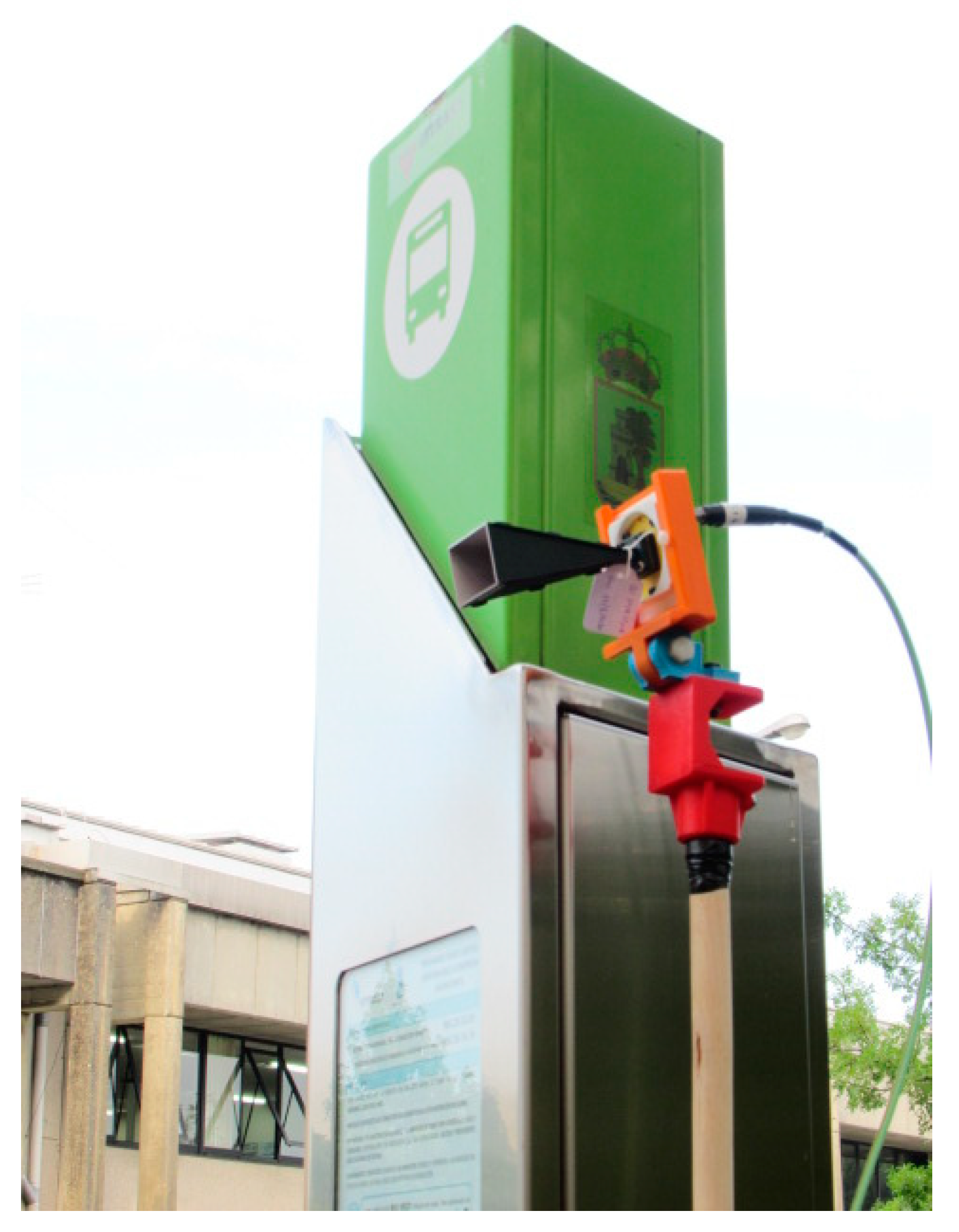
2. Experimental Set-Up
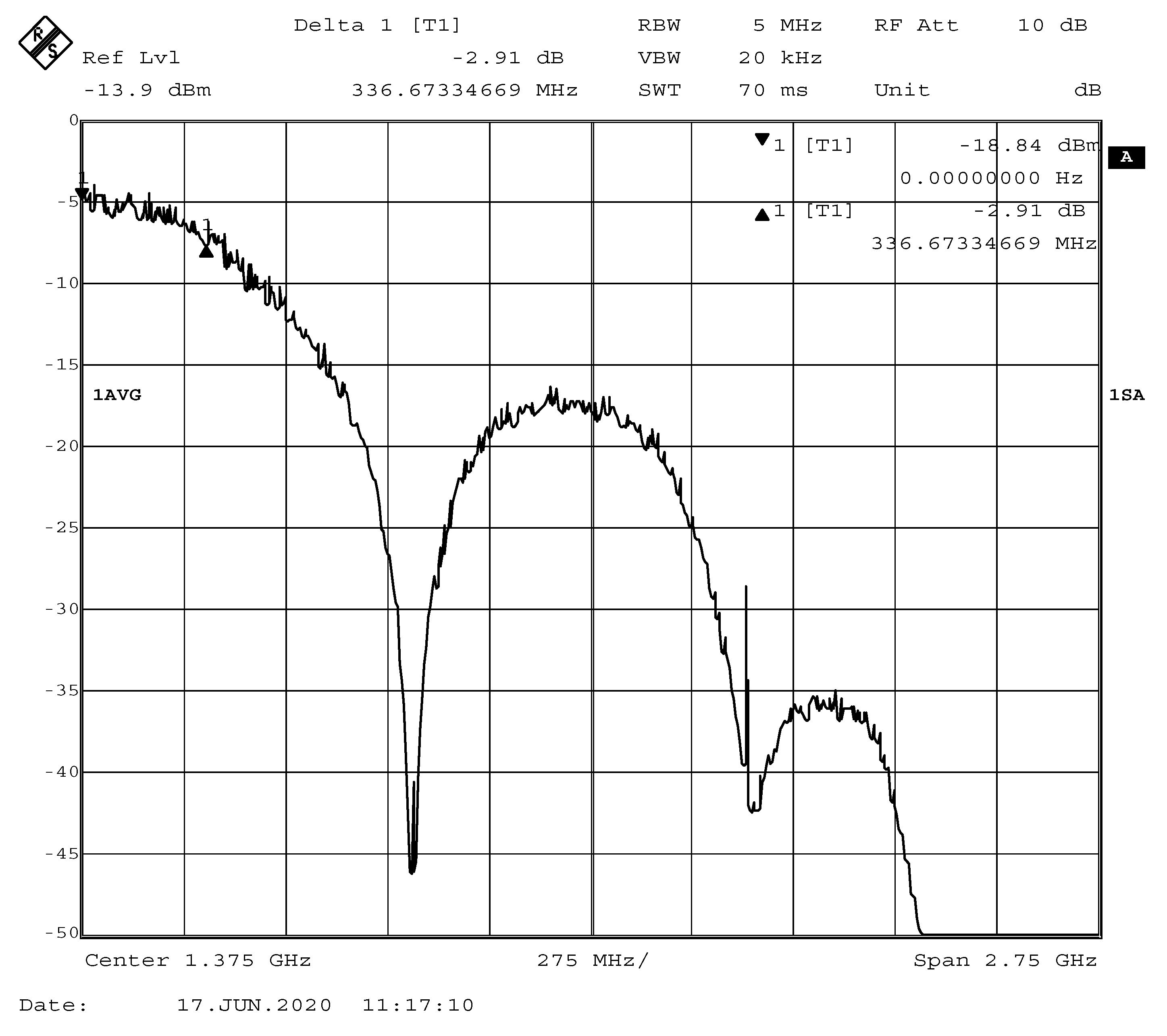
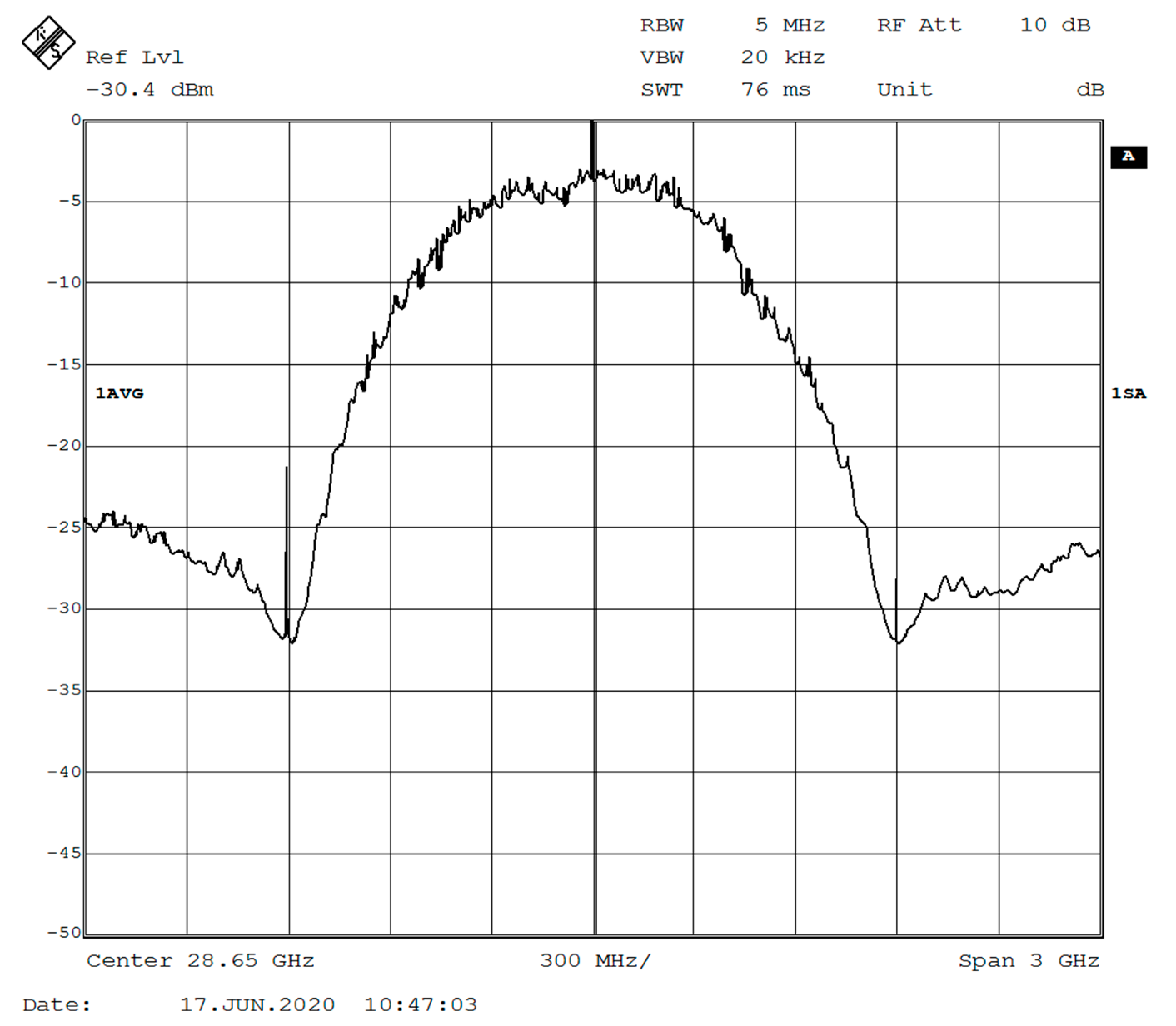
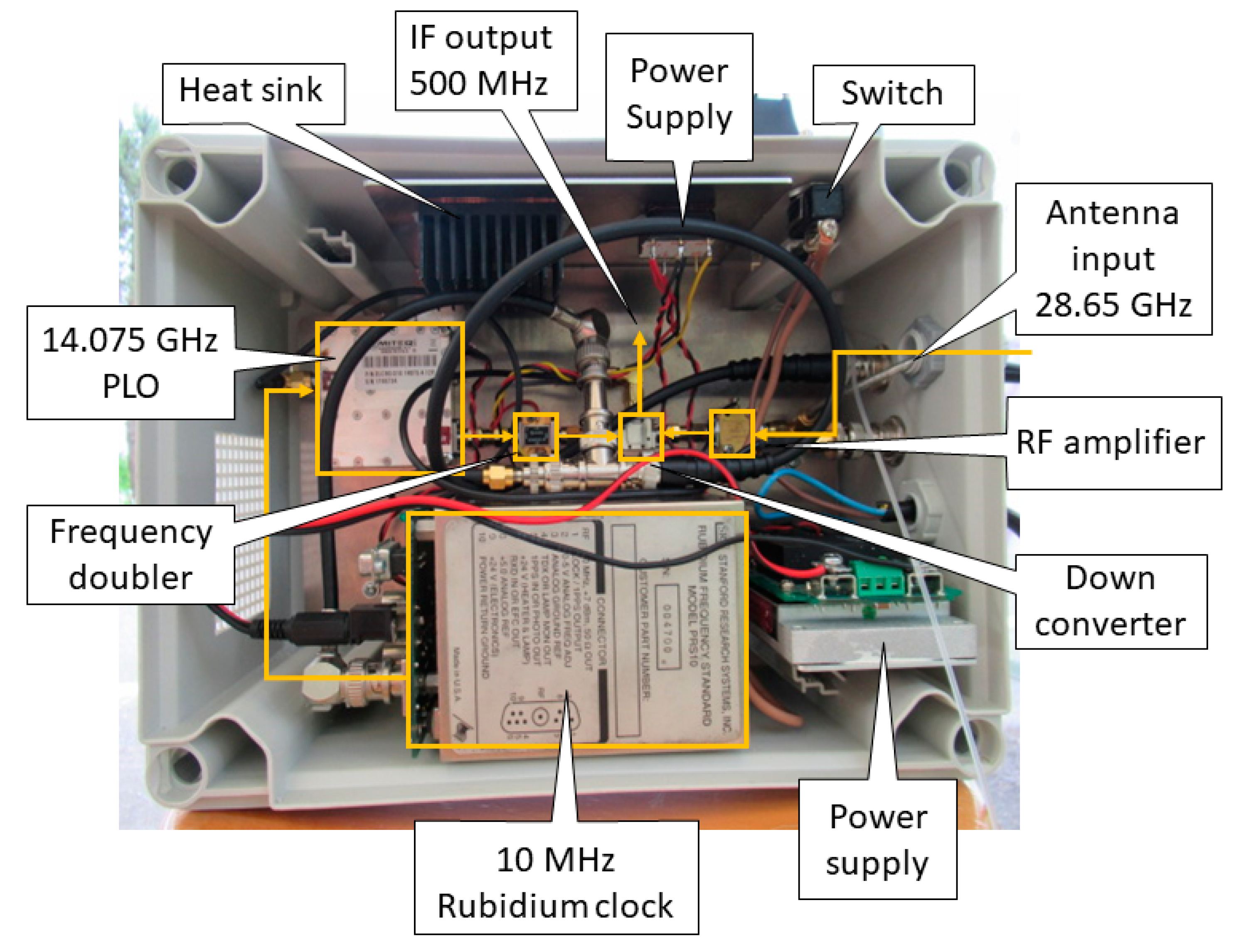
2.1. Channel Sounder
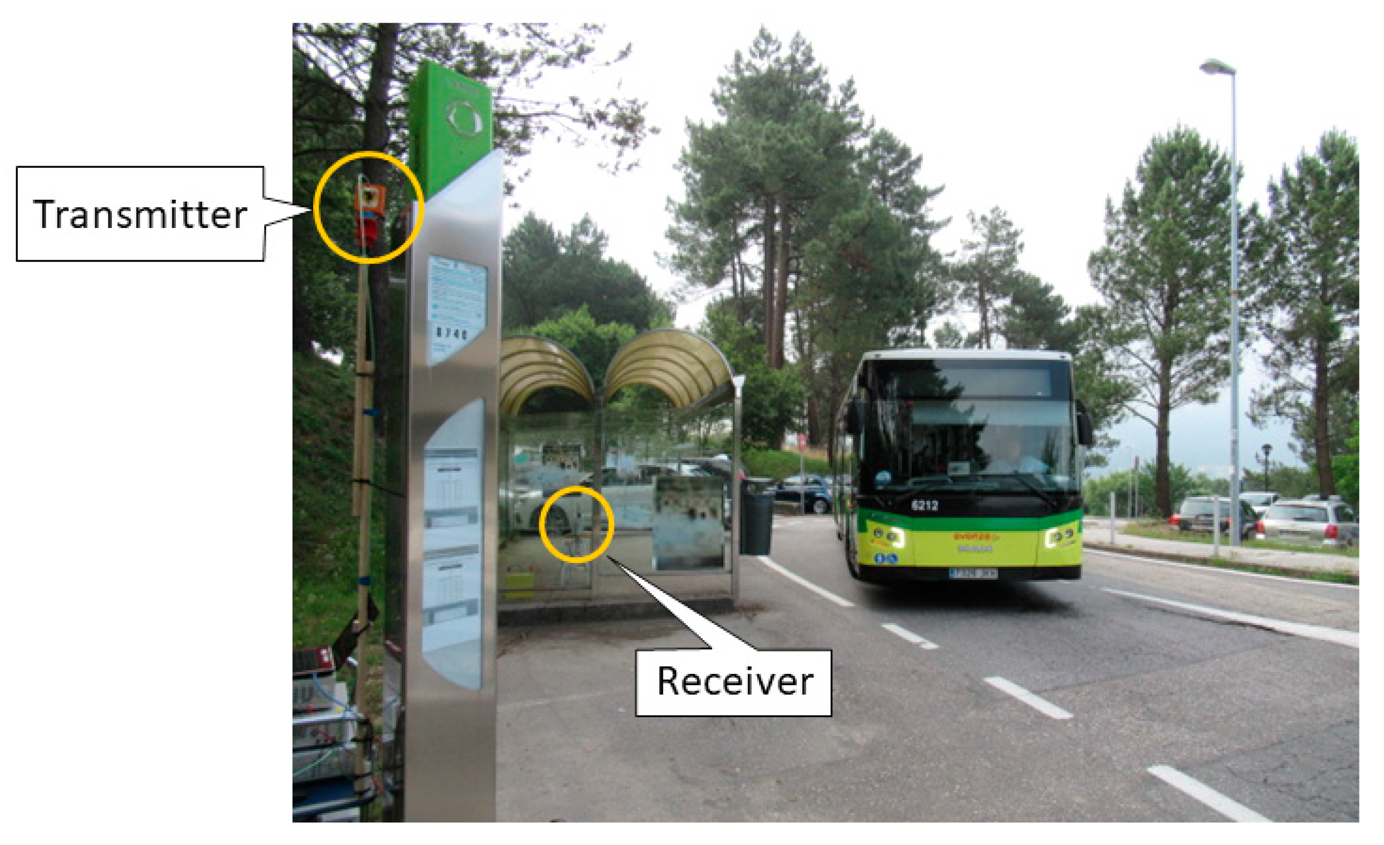
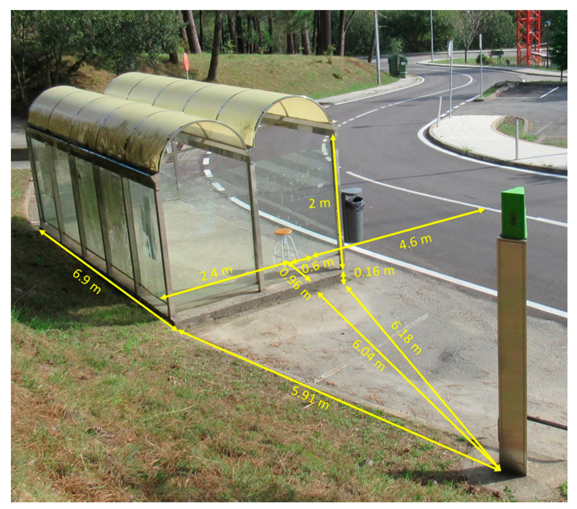
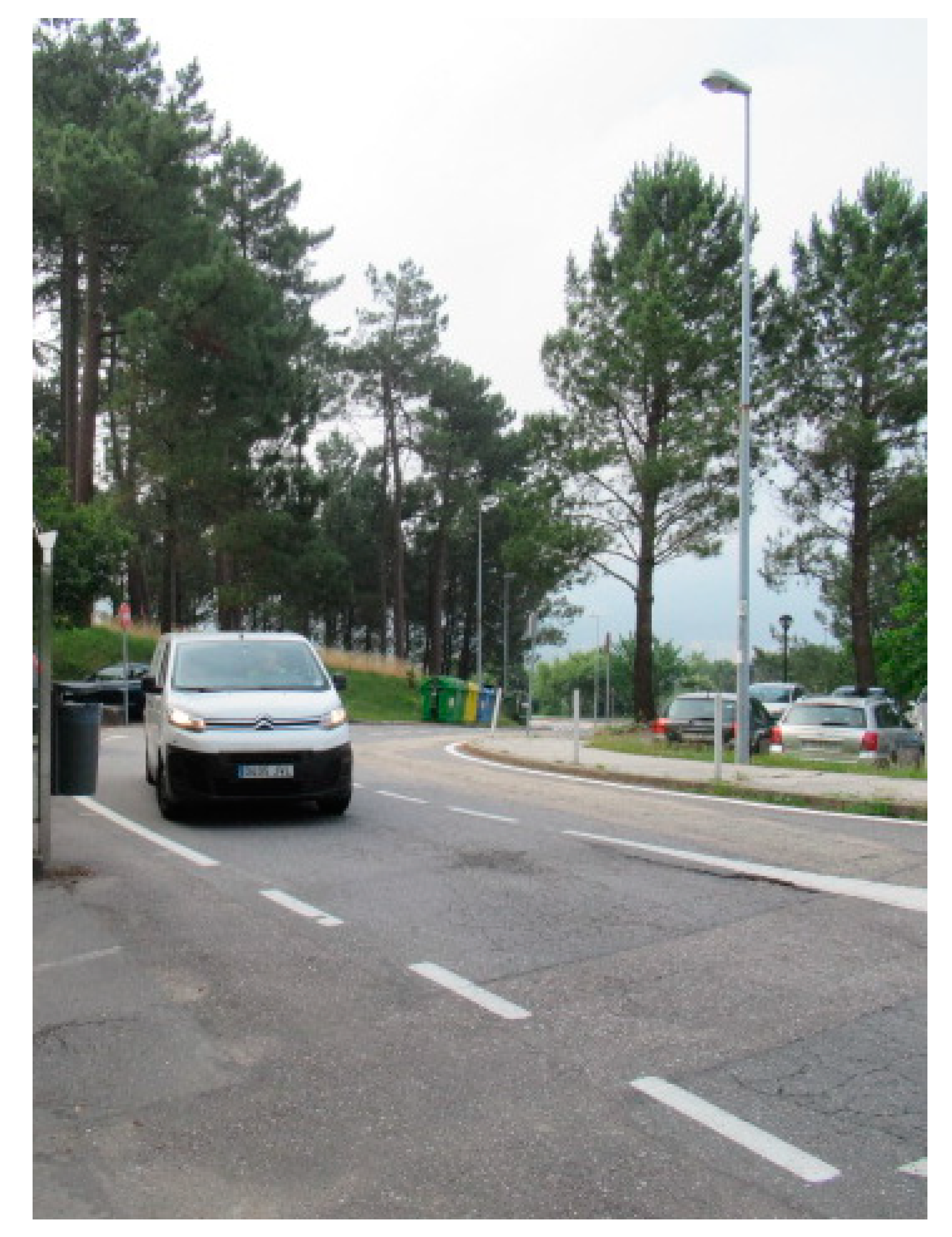
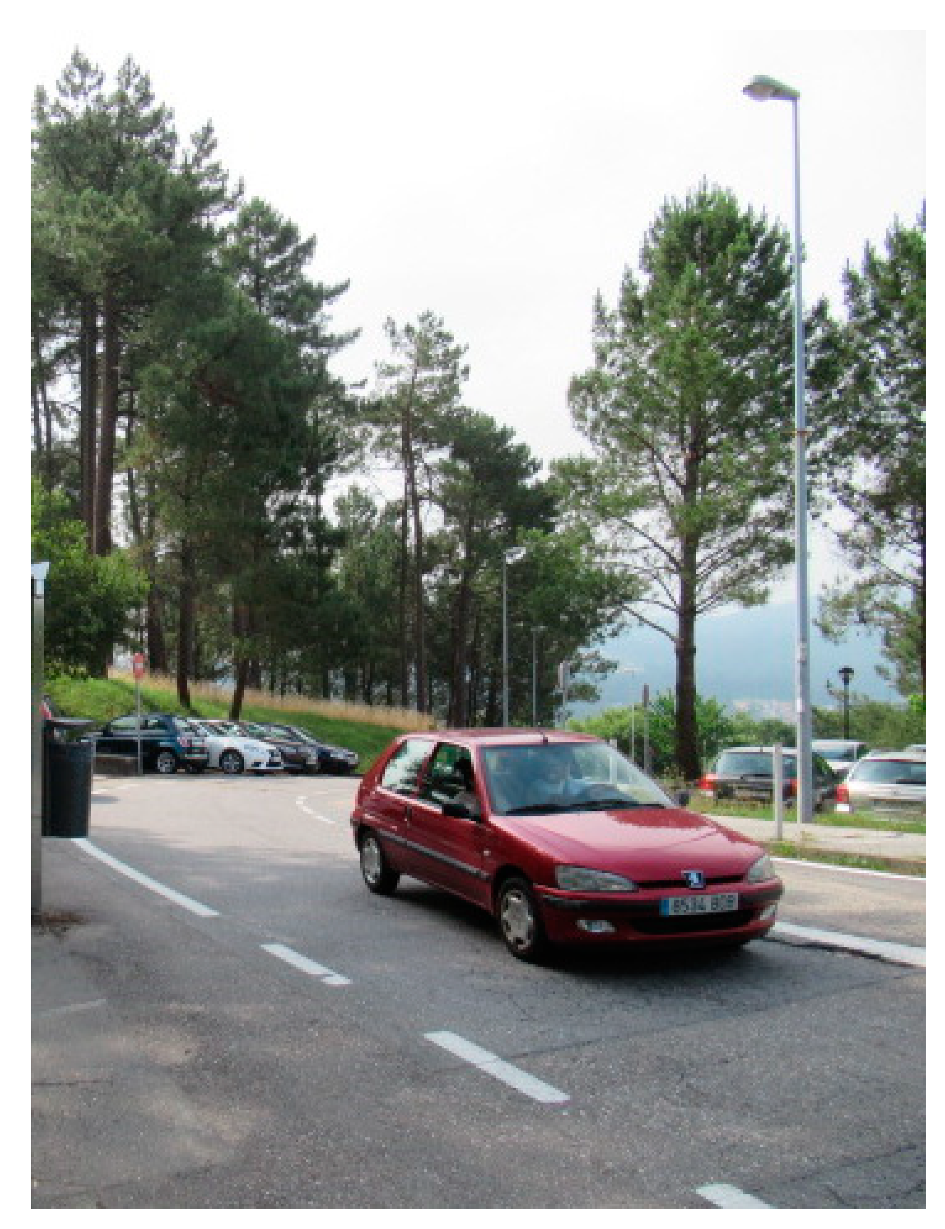
2.2. Measurement Scenario
2.3. Data Processing
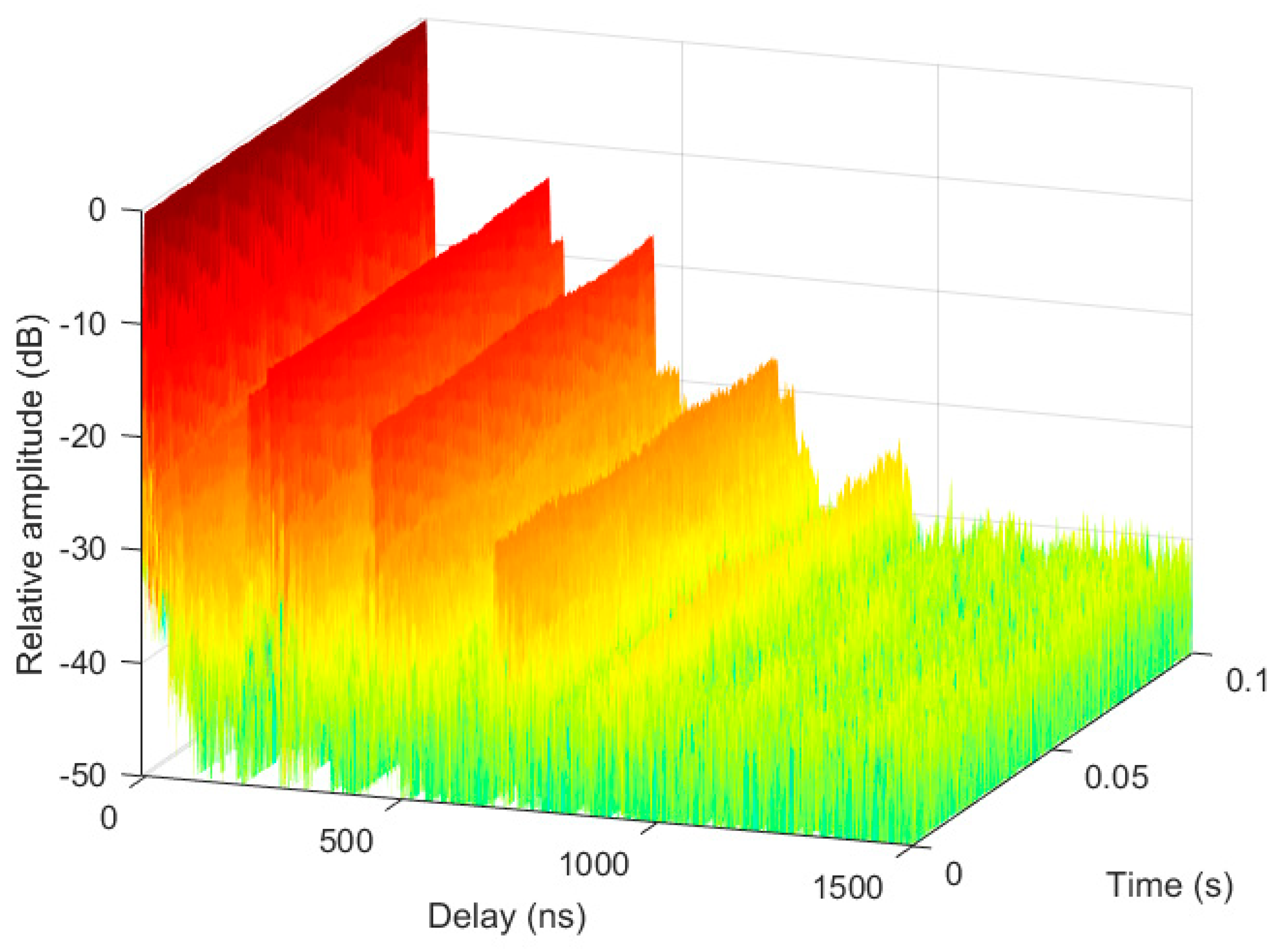
3. Results
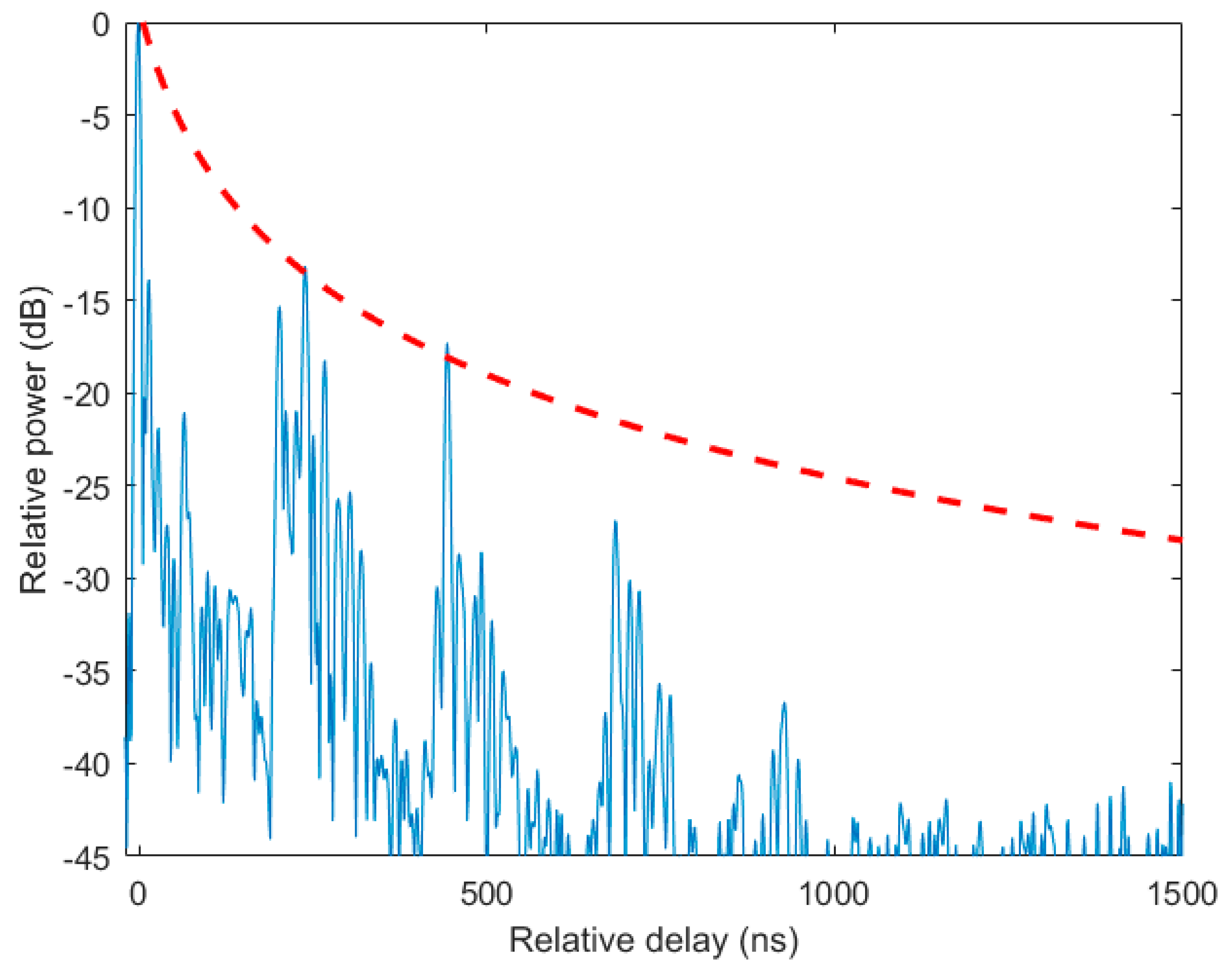
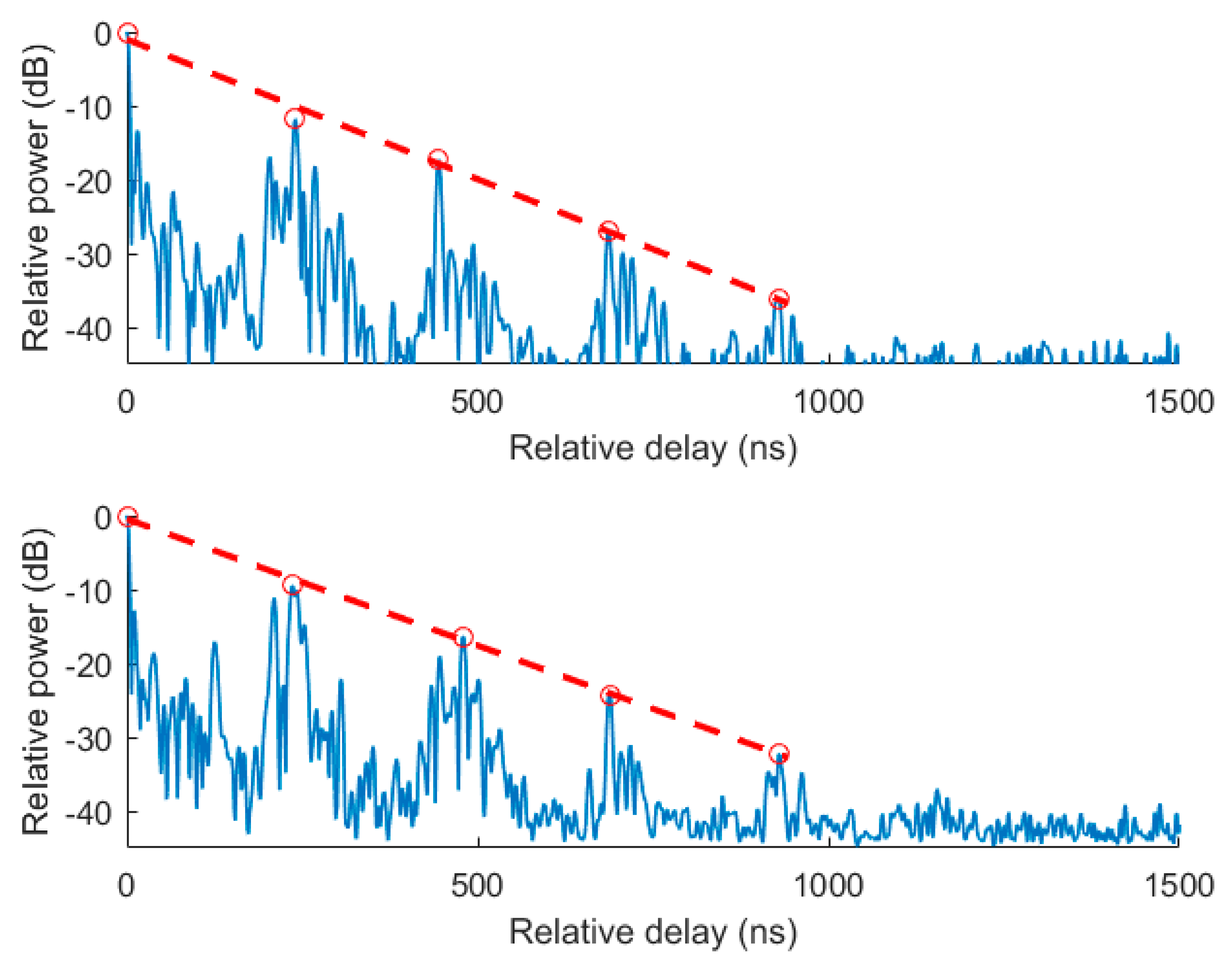
3.1. Delay Spread
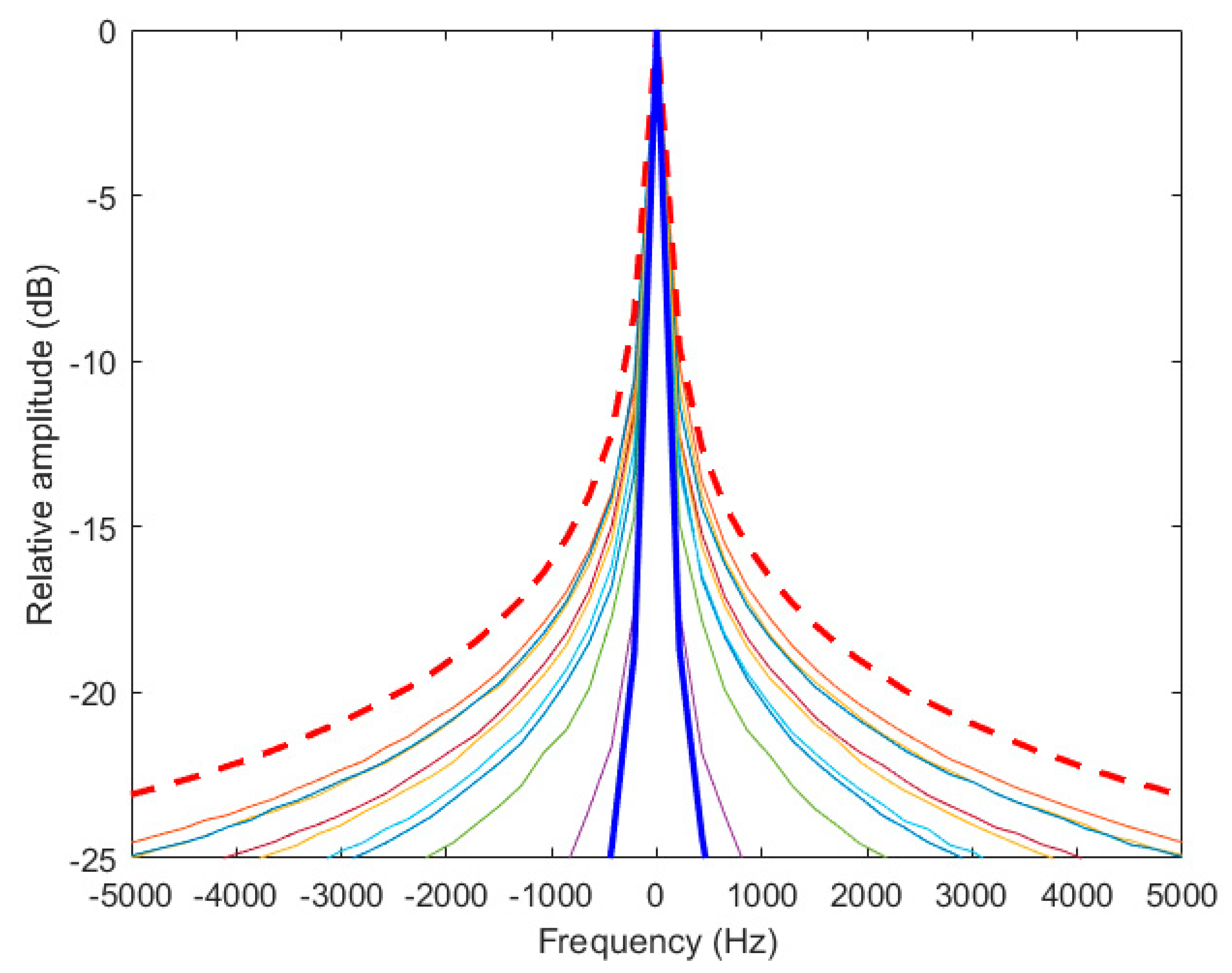
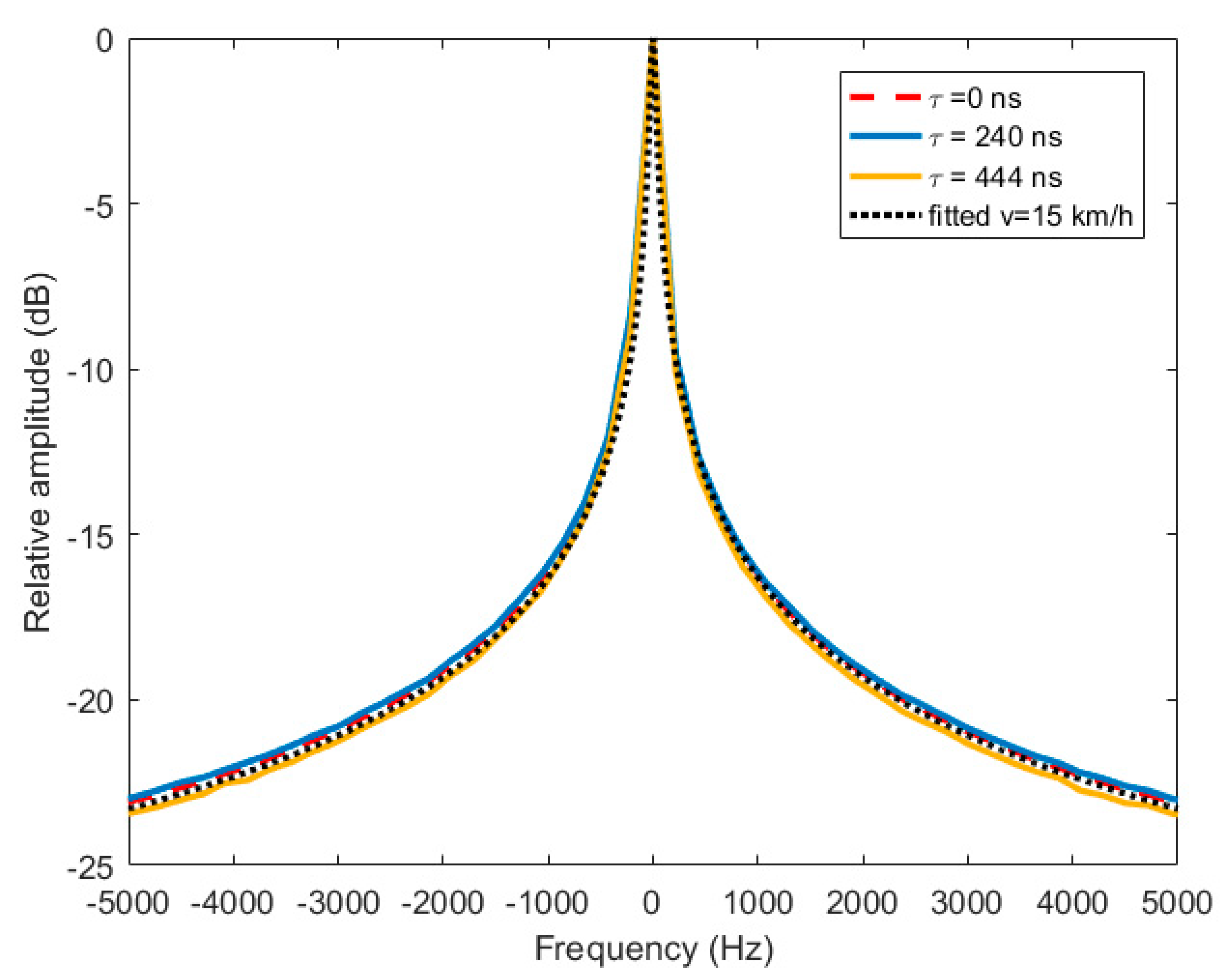
3.2. Doppler Spectrum
4. Conclusions
Author Contributions
Funding
Conflicts of Interest
References
- GSMA Intelligence. Understanding 5G: Perspectives on Future Technological Advancements in Mobile; GSMA Intelligence: London, UK, 2014. [Google Scholar]
- Andrews, J.G.; Buzzi, S.; Choi, W.; Hanly, S.V.; Lozano, A.; Soong, A.C.; Zhang, J.C. What will 5G be? IEEE J. Sel. Areas Commun. 2014, 32, 1065–1082. [Google Scholar] [CrossRef]
- Sánchez, M.G.; Portela, M.; Lemos, E. Millimeter wave radio channel characterization for 5G vehicle-to-vehicle communications. Measurement 2017, 95, 223–229. [Google Scholar] [CrossRef]
- International Wireless Industry Consortium. Evolutionary & Disruptive Visions towards Ultra High Capacity Networks White Paper; International Wireless Industry Consortium: Doylestown, PA, USA, 2014. [Google Scholar]
- Valliappan, N.; Lozano, A.; Heath, R.W. Antenna Subset Modulation for Secure Millimeter-Wave Wireless Communication. IEEE Trans. Commun. 2013, 61, 3231–3245. [Google Scholar] [CrossRef]
- IEEE Std 802.11ad-2012: Part 11: Wireless LAN Medium Access Control (MAC) and Physical Layer (PHY) Specifications: Amendment 3: Enhancements for Very High Throughput in the 60 GHz Band; IEEE Computer Society: Washington, DC, USA, 2012.
- El Ayach, O.; Heath, R.W.; Abu-Surra, S.; Rajagopal, S.; Pi, Z. The capacity optimality of beam steering in large millimeter wave. In Proceedings of the IEEE 13th International Workshop on Signal Processing Advances in Wireless Communications (SPAWC), Cesme, Turkey, 17–20 June 2012; pp. 100–104. [Google Scholar]
- Kumari, P.; Gonzalez-Prelcic, N.; Heath, R.W. Investigating the IEEE 802.11ad Standard for Millimeter Wave Automotive Radar. In Proceedings of the IEEE 82nd Vehicular Technology Conference (VTC Fall), Boston, MA, USA, 6–9 September 2015. [Google Scholar]
- Murad, N.A.; Raja Suleiman, R.F. Design of a ridged waveguide slot antenna for millimeterwave applications. In Proceedings of the IEEE International RF and Microwave Conference (RFM), Seremban, Negeri Sembilan, 12–14 December 2011; pp. 205–208. [Google Scholar]
- Steele, R. Mobile Radio Communications; Wiley-Blackwell: Hoboken, NJ, USA, 1992. [Google Scholar]
- Saad, W.; Bennis, M.; Chez, M. A vision of 5G wireless systems: Applications, trends, technologies, and open research problems. IEEE Netw. 2020, 34, 134–142. [Google Scholar] [CrossRef]
- Busari, S.A.; Mumtaz, S.; Al-Rubaye, A.; Rodríguez, J. 5G millimeter-wave mobile broadband: Performance and challenges. IEEE Commun. Mag. 2018, 56, 137–143. [Google Scholar] [CrossRef]
- Small Cells Forum. Available online: www.smallcellforum.org (accessed on 22 September 2020).
- Cox, D. Delay Doppler characteristics of multipath propagation at 910 MHz in a suburban mobile radio environment. IEEE Trans. Antennas Propag. 1972, 20, 625–635. [Google Scholar] [CrossRef]
- Baum, D.S.; Gore, D.; Nabar, R.; Panchanathan, S.; Hari, K.V.S.; Erceg, V.; Paulraj, A.J. Measurement and characterization of broadband MIMO fixed wireless channels at 2.5 GHz. In Proceedings of the 2000 IEEE International Conference on Personal Wireless Communications, Hyderabad, India, 17–20 December 2000; pp. 203–206. [Google Scholar]
- Torres, R.P.; Cobo, B.; Mavares, D.; Medina, D.; Loredo, S.; Engels, M. Measurement and statistical analysis of the temporal variations of a fixed wireless link at 3.5 GHz. Wirel. Pers. Commun. 2006, 37, 41–59. [Google Scholar] [CrossRef]
- Domazetovic, A.; Greenstein, L.J.; Mandayam, N.B.; Seskar, I. Estimating the Doppler spectrum of a short-range fixed wireless channel. IEEE Commun. Lett. 2003, 7, 227–229. [Google Scholar] [CrossRef]
- Naz, N.; Falconer, D.D. Temporal variations characterization for fixed wireless at 29.5 GHz. In Proceedings of the 2000 IEEE 51st Vehicular Technology Conference Proceedings, Tokyo, Japan, 15–18 May 2000; pp. 2178–2182. [Google Scholar]
- Sánchez, M.G.; Lemos, E.; Alejos, A.V. Empirical modeling of radiowave angular power distributions in different propagation environments at 60 GHz for 5G. Electronics 2018, 7, 365. [Google Scholar] [CrossRef]
- METIS. METIS Channel Models. ICT-317669 METIS Project. 2015. Available online: https://metis2020.com/documents/deliverables/METIS_D1.4_v1.0.pdf (accessed on 31 August 2020).
- Medbo, J.; Kyosti, P.; Kusume, K.; Raschkowski, L.; Haneda, K.; Jamsa, T.; Nurmela, V.; Roivainen, A.; Meinila, J. Radio propagation modeling for 5G mobile and wireless communications. IEEE Commun. Mag. 2016, 54, 144–151. [Google Scholar] [CrossRef]
- Liu, L.; Oestges, C.; Poutanen, J.; Haneda, K.; Vainikainen, P.; Quitin, F.; Tufvesson, F.; de Doncker, P. The COST 2100 MIMO channel model. IEEE Wirel. Commun. Mag. 2012, 19, 92–99. [Google Scholar] [CrossRef]
- Meinila, J.; Kyosti, P.; Hentila, L.; Jamsa, T.; Suikkanen, E.; Kunnari, E.; Narandzic, M. D5.3: WINNER+ Final Channel Models. Wirel. World Initiat. New Radio 2010, 119–172. Available online: https://docplayer.net/34577643-D5-3-winner-final-channel-models.html (accessed on 22 September 2020).
- ETSI TR 138 900 V14.3.1 Study on Channel Model for Frequency Spectrum above 6 GHz (3GPP TR 38.900 Version 14.3.1 Release 14). Available online: https://cdn.standards.iteh.ai/samples/53521/f79aa5eea08c43c1b6cc18f62baa26af/ETSI-TR-138-900-V14-3-1-2017-08-.pdf (accessed on 22 September 2020).
- Saleh, A.A.M.; Valenzuela, R. A statistical model for indoor multipath propagation. IEEE J. Sel. Areas Commun. 1987, 5, 128–137. [Google Scholar] [CrossRef]
- Channel Models for IEEE 802.11ay, doc IEEE 802.11-15/1150r9. May 2016. Retrieved on 1st September 2020. Available online: https://www.ieee802.org/11/Reports/tgay_update.htm (accessed on 22 September 2020).
- Weiler, R.J.; Peter, M.; Keusgen, W.; Maltsev, A.; Karls, I.; Pudeyev, A.; Bolotin, I.; Siaud, I.; Ulmer-Moll, A.M. Quasi-deterministic millimeter-wave channel models in MiWEBA. EURASIP J. Wirel. Commun. Netw. 2016, 2016, 84–99. [Google Scholar] [CrossRef]
- Shiu, D.-S.; Foschini, G.J.; Gans, M.J.; Kahn, J.M. Fading correlation and its effect on the capacity of multielement antenna systems. IEEE Trans. Commun. 2000, 48, 502–513. [Google Scholar] [CrossRef]
- Borhani, A.; Pätzold, M. A unified disk scattering model and its angle-of-departure and time-of-arrival statistics. IEEE Trans. Veh. Technol. 2013, 62, 473–485. [Google Scholar] [CrossRef]
- Liberti, J.C.; Rappaport, T.S. A geometrically based model for line-of-sight multipath radio channels. In Proceedings of the Vehicular Technology Conference-VTC, Atlanta, GA, USA, 28 April–1 May 1996; pp. 844–848. [Google Scholar]
- Patzold, M.; Hogstad, B.O. A wideband MIMO channel model derived from the geometric elliptical scattering model. In Proceedings of the 3rd International Symposium on Wireless Communication Systems (ISWCS), Valencia, Spain, 5–8 September 2006; pp. 138–143. [Google Scholar]
- Borhani, A.; Pätzold, M. Correlation and spectral properties of vehicle-to-vehicle channels in the presence of moving scatterers. IEEE Trans. Veh. Technol. 2013, 62, 4228–4239. [Google Scholar] [CrossRef]
- Zhao, X.; Han, Q.; Li, B.; Dou, J.; Hong, W. Doppler spectra for F2F radio channels with moving scaterrers. IEEE Trans. Antennas Propagat. 2016, 64, 4107–4112. [Google Scholar] [CrossRef]
- Andersen, J.B.; Nielsen, J.O.; Pedersen, J.O.; Bauch, G.; Dietl, G. Doppler spectrum from moving scatterers in a random environment. IEEE Trans. Wirel. Commun. 2009, 8, 3270–3277. [Google Scholar] [CrossRef]
- Bian, J.; Sun, J.; Wang, C.X.; Feng, R.; Huang, J.; Yang, Y.; Zhang, M. A Winner+ based 3D non-stationary wideband MIMO channel model. IEEE Trans. Wirel. Commun. 2018, 17, 1755–1767. [Google Scholar] [CrossRef]
- Lorca, J.; Hunukumbure, M.; Wang, Y. On overcoming the impact of Doppler spectrum in millimeter-wave V2I communications. In Proceedings of the IEEE Globecom Workshops, Singapore, 4–8 December 2017. [Google Scholar]
- Pedersen, K.I.; Mogensen, P.E.; Fleury, B.H. A stochastic model of the temporal and azimuthal dispersion seen at the base station in outdoor propagation environments. IEEE Trans. Veh. Technol. 2000, 49, 437–447. [Google Scholar] [CrossRef]
- Sanchez, M.G.; De Haro, L.; Pino, A.G.; Calvo, M. Human operator effect on wide band radio channel characteristics. IEEE Trans. Antennas Propag. 1997, 45, 1318–1320. [Google Scholar] [CrossRef]


© 2020 by the authors. Licensee MDPI, Basel, Switzerland. This article is an open access article distributed under the terms and conditions of the Creative Commons Attribution (CC BY) license (http://creativecommons.org/licenses/by/4.0/).
Share and Cite
García Sánchez, M.; Santomé Valverde, A.; Expósito, I. Radio Channel Scattering in a 28 GHz Small Cell at a Bus Stop: Characterization and Modelling. Electronics 2020, 9, 1556. https://doi.org/10.3390/electronics9101556
García Sánchez M, Santomé Valverde A, Expósito I. Radio Channel Scattering in a 28 GHz Small Cell at a Bus Stop: Characterization and Modelling. Electronics. 2020; 9(10):1556. https://doi.org/10.3390/electronics9101556
Chicago/Turabian StyleGarcía Sánchez, Manuel, Alejandro Santomé Valverde, and Isabel Expósito. 2020. "Radio Channel Scattering in a 28 GHz Small Cell at a Bus Stop: Characterization and Modelling" Electronics 9, no. 10: 1556. https://doi.org/10.3390/electronics9101556
APA StyleGarcía Sánchez, M., Santomé Valverde, A., & Expósito, I. (2020). Radio Channel Scattering in a 28 GHz Small Cell at a Bus Stop: Characterization and Modelling. Electronics, 9(10), 1556. https://doi.org/10.3390/electronics9101556