Q-Learning of Straightforward Gait Pattern for Humanoid Robot Based on Automatic Training Platform

Abstract

In this paper, an oscillator-based gait pattern with sinusoidal functions is designed and implemented on a field-programmable gate array (FPGA) chip to generate a trajectory plan and achieve bipedal locomotion for a small-sized humanoid robot. In order to let the robot can walk straight, the turning direction is viewed as a parameter of the gait pattern and Q-learning is used to obtain a straightforward gait pattern. Moreover, an automatic training platform is designed so that the learning process is automated. In this way, the turning direction can be adjusted flexibly and efficiently under the supervision of the automatic training platform. The experimental results show that the proposed learning framework allows the humanoid robot to gradually walk straight in the automated learning process.

1. Introduction

Humanoid robots are an attractive topic in the field of robotics. A biped structure is designed for humanoid robots and is expected to facilitate human lives and even allow the robots to coexist with humans. Therefore, bipedal locomotion is an important ability of humanoid robots that is widely researched. Some gait patterns are motivated by biologically inspired control concepts to achieve bipedal locomotion. Rhythmic movements in animals are realized via an interaction between the dynamics of a musculoskeletal system and the rhythmic signals from central pattern generators (CPGs) [1,2]. In robotics, CPGs were formulated as a set of neural oscillators to produce the gait pattern of oscillations necessary for rhythmic movements [3,4]. Based on the neural oscillator, a set of coupled-phase oscillators were presented using sinusoidal functions for the gait pattern [5]. However, the neural oscillator and the coupled-phase oscillator are modulated in the joint space for each joint of the humanoid robot, resulting in too many parameters needing to be adjusted. Based on the Cartesian coordinate system, the simplified coupled linear oscillators were extended from the abovementioned methods to produce the gait pattern [6,7] with trajectory planning in the workspace [8,9]. The simplified coupled linear oscillators can be divided into a balance oscillator and two movement oscillators which have a direct correlation between the oscillator parameters and the gait pattern. The center of mass (CoM) trajectory can be designed through the balance oscillator and its oscillator parameters. Similarly, the left and right ankle trajectories can be designed through the movement oscillator and its oscillator parameters. Hence, these oscillator parameters all affect the gait pattern for the humanoid robot. This gait pattern for the humanoid robot can achieve high flexibility through adjustment of the parameters of the oscillator-based gait pattern. Inverse kinematics [10] was performed to transform trajectory planning into the desired joint position, and the gait pattern of the humanoid robot can be implemented to achieve bipedal locomotion.

The ability to improve the desired behavior of the robot is a significant technical challenge. The dynamic motion problems could be solved for unmanned aerial vehicles (UAVs) [11], quadruped robots [12], and even high-dimensional humanoid robots [13] using the Q-learning algorithm [14,15,16]. Most gait patterns are designed for humanoid robots, assuming an ideal situation. However, in the long-term operation of the humanoid robot, some errors may accumulate owing to mechanism error and motor backlash. Moreover, the real environment may also result in the humanoid robot exhibiting some unexpected behaviors. In order to adapt environmental changes through the gait pattern of the humanoid robot, sensors are needed to obtain environmental information [17,18,19]. The desired behavior of the robot can be learned to appropriately modulate the observed gait pattern [20,21,22,23]. Hence, some studies were developed to adjust the joints [24,25] of the humanoid robot based on the interaction between the robot and the environment. The angle at each joint can be calculated and rotated to simulate the straightforward gait pattern. Furthermore, some studies were developed to adjust the poses [26] of the humanoid robot in order to speed up the learning process. The robot poses are formed by a set of gait patterns to avoid the complex adjustment of multiple joints and to further implement the straightforward gait pattern. Hence, the straightforward gait pattern is learned for the humanoid robot by adjusting the gait pattern with environmental information.

In most cases, for humanoid robots, the simulation results are adequate, but it is difficult to directly apply the calculated data to real humanoid robots owing to the possibility of mechanism error and motor backlash. Therefore, this paper focuses on an experiment to allow a real robot to successfully learn the desired behavior. In this paper, a learning framework is proposed for the humanoid robot to efficiently learn a straightforward walking gait in a real-life situation. In order to reduce the number of learning parameters, an oscillator-based gait pattern with sinusoidal functions is designed so that it can simultaneously speed up the learning process and make the gait pattern more flexible to achieve bipedal locomotion. In this paper, only the turning direction (the parameter of the gait pattern) needs to be learned by the Q-learning algorithm to obtain a straightforward gait pattern. Moreover, in order to reduce the level of human resources and to protect the humanoid robot, an automatic training platform, as an auxiliary function, is designed to effectively assist and supervise the intrinsically unstable humanoid robot. The automatic training platform can also be applied to collect environmental information for the humanoid robot to adjust the turning direction. The oscillator-based gait pattern and the Q-learning algorithm are deployed on a field-programmable gate array (FPGA) chip. Hence, it can be integrated with an automatic training platform in the proposed learning framework such that the adaptability of the humanoid robot can be improved and the straightforward gait pattern can also be learned.

The rest of this paper is organized as follows: in Section 2, the structure and specification of a small-sized humanoid robot and the automatic training platform used in the experiment are described. In Section 3, the system architecture and system process of the proposed learning framework based on the FPGA chip and the automatic training platform are described. In Section 4, an oscillator-based gait pattern is designed for the humanoid robot using trajectory planning. A balance oscillator and two movement oscillators are generated, allowing a direct correlation between oscillator parameters and the gait pattern. In Section 5, the Q-learning algorithm is presented with the proposed automatic training platform for the humanoid robot to learn the straightforward gait pattern. In Section 6, some experimental results are presented to validate the proposed learning framework. Finally, the conclusions are summarized in Section 7.

2. Hardware Structure and Coordinate System

In this paper, a small-sized humanoid robot and the automatic training platform developed by our laboratory (Intelligent Control Laboratory of Tamkang University) are shown in Figure 1; this experimental platform was designed to implement the proposed method and achieve the desired behavior of the robot.

2.1. Small-Sized Humanoid Robot

A small-sized humanoid robot with 23 degrees of freedom (DOFs) was designed to imitate human movements. There were two DOFs in the head, four DOFs per arm, one DOF in the waist, and six DOFs per leg. The mechanism and dimensions of the small-sized humanoid robot are described in Figure 2. Its height and weight were 56.45 cm and 4.5 kg, respectively. The main hardware included 23 servo motors, one complementary metal–oxide–semiconductor (CMOS) sensor, one FPGA board, and one integrated circuit board. The specifications of the small-sized humanoid robot are shown in

Table 1. Specifications of the small-sized humanoid robot.

Category	Description	Data
Dimension	Height Weight	56.45 cm 5.34 kg
DOFs	Head Arm Waist Leg	2 DOFs 4 DOFs × 2 1 DOF 6 DOFs × 2
Main controller (FPGA)	CPU RAM Logic gates Power requirement	Altera Cyclone III EP3C120F780C8 DDRII SDRAM 64 MB × 2 119088 1 DC power jack with 5 V power input
Actuator MX-28 (arm)	Holding torque Speed Resolution	2.5 N∙m @ 12 V 55 rpm @ no load 0.088°
Actuator MX-64 (leg)	Holding torque Speed Resolution	6.0 N∙m @ 12 V 63 rpm @ no load 0.088°
Sensor	CMOS sensor	30 fps

. The FPGA board contained an FPGA chip which was used as the main controller for the humanoid robot. The internal signals of the robot could be transferred into the FPGA chip through the integrated circuit board. Hence, the commands could be transmitted from the FPGA chip to all device components (i.e., the 23 servo motors) by using general-purpose input/output (GPIO) pins and the integrated circuit board. It can be mentioned that the FPGA chip has the advantage of parallel processing and low power consumption. Therefore, the small-sized humanoid robot designed with this FPGA board had more significant computing and real-time processing capabilities compared to the Darwin-OP robot [6] with an Arduino board.

In this paper, trajectory planning was adopted to achieve the gait pattern of the humanoid robot. Hence, inverse kinematics was applied to obtain the angle of each joint from the trajectory planning to implement bipedal locomotion. The geometric approach was used to solve the inverse kinematics. The coordinate systems of the humanoid robot described in its sagittal plane and frontal plane are shown in Figure 3 [10].

In the sagittal plane of the humanoid robot described in Figure 3a, the angles of the hip joint, knee joint, and ankle joint of the right (left) foot in the pitch-axis are denoted as ${\theta }_{RH}^{pit}$(${\theta }_{LH}^{pit}$), ${\theta }_{RK}^{pit}$(${\theta }_{LK}^{pit}$), and ${\theta }_{RA}^{pit}$(${\theta }_{LA}^{pit}$), respectively. Based on the geometric approach, ${\theta }_{RH}^{pit}$, ${\theta }_{RK}^{pit}$, ${\theta }_{RA}^{pit}$, ${\theta }_{LH}^{pit}$, ${\theta }_{LK}^{pit}$, and ${\theta }_{LA}^{pit}$ can be respectively described as follows:

$${\theta }_{RH}^{pit}={\cos }^{-1}(\frac{L_R^x{}^2+L_R^z{}^2+l_t{}^2-l_c{}^2}{2l_t\sqrt{L_R^x{}^2+L_R^z{}^2}})+{\tan }^{-1}(\frac{L_R^x}{L_R^z}),$$

(1)

$${\theta }_{RK}^{pit}=\pi -{\tan }^{-1}(\frac{l_t\cos ({\theta }_{RH}^{pit})}{l_t\sin ({\theta }_{RH}^{pit})})-{\tan }^{-1}(\frac{L_R^z-l_t\cos ({\theta }_{RH}^{pit})}{l_t\sin ({\theta }_{RH}^{pit})-L_R^x}),$$

(2)

$${\theta }_{RA}^{pit}={\tan }^{-1}(\frac{l_t\sin ({\theta }_{RH}^{pit})-L_R^x}{L_R^z-l_t\cos ({\theta }_{RH}^{pit})}),$$

(3)

$${\theta }_{LH}^{pit}={\cos }^{-1}(\frac{L_L^x{}^2+L_L^z{}^2+l_t{}^2-l_c{}^2}{2l_t\sqrt{L_L^x{}^2+L_L^z{}^2}})+{\tan }^{-1}(\frac{L_L^x}{L_L^z}),$$

(4)

$${\theta }_{LK}^{pit}=\pi -{\tan }^{-1}(\frac{l_t\cos ({\theta }_{LH}^{pit})}{l_t\sin ({\theta }_{LH}^{pit})})-{\tan }^{-1}(\frac{L_L^z-l_t\cos ({\theta }_{LH}^{pit})}{l_t\sin ({\theta }_{LH}^{pit})-L_L^x}),$$

(5)

and

$${\theta }_{LA}^{pit}={\tan }^{-1}(\frac{l_t\sin ({\theta }_{LH}^{pit})-L_L^x}{L_L^z-l_t\cos ({\theta }_{LH}^{pit})}),$$

(6)

where $l_t$ and $l_c$ are the lengths of the robot thigh and calf, respectively. $L_R^x$($L_L^x$), $L_R^y$($L_L^y$), and $L_R^z$($L_L^z$) are the step length, step width, and lift height of the right (left) foot.

In the frontal plane of the humanoid robot described in Figure 3b, the angles of the hip joint and ankle joint of the right (left) foot in the roll axis are denoted as ${\theta }_{RH}^{rol}$(${\theta }_{LH}^{rol}$) and ${\theta }_{RA}^{rol}$(${\theta }_{LA}^{rol}$), respectively. Similarly, based on the geometric approach, ${\theta }_{RH}^{rol}$, ${\theta }_{RA}^{rol}$, ${\theta }_{LH}^{rol}$, and ${\theta }_{LA}^{rol}$ can be respectively described as follows:

$${\theta }_{RH}^{rol}={\sin }^{-1}(\frac{L_R^y}{L_R^z}),$$

(7)

$${\theta }_{RA}^{rol}={\theta }_{RH}^{rol},$$

(8)

$${\theta }_{LH}^{rol}={\sin }^{-1}(\frac{L_L^y}{L_L^z}),$$

(9)

and

$${\theta }_{LA}^{rol}={\theta }_{LH}^{rol}.$$

(10)

2.2. Automatic Training Platform

An automatic training platform with three degrees of freedom was designed to allow the robot to be trained in an automated learning process. The specifications of the automatic training platform are shown in

Table 2. Specifications of the automatic training platform.

Category	Description	Data
Dimension	Length Width Height	243 cm 124 cm 85 cm
DOFs	Platform	3 DOFs
Main controller (PC)	CPU RAM	Intel i5-5200U 8 GB DDR3 SDRAM
Actuator MX-64	Holding torque Speed Resolution	6.0 N∙m @ 12 V 63 rpm @ no load 0.088°
Sensors	Infrared sensor CMOS sensor	x-axis/y-axis 30 fps

. The main hardware included three servo motors, one personal computer (PC), two infrared sensors, and one CMOS sensor. The PC was used as the main controller for the automatic training platform. The mechanism dimension of the automatic training platform is shown in Figure 4. Its length, width, and height were 243 cm, 124 cm, and 85 cm, respectively. The length and width of the training field were 238 cm and 119 cm, respectively. Two infrared sensors were used to measure x-axis and y-axis distances of the robot in the training field. As shown in Figure 5, a unit coordinate of 17 × 17 cm² was considered to construct the coordinate of the training field in the horizontal plane of the automatic training platform. The measured information ($d_x$, $d_y$) was transferred into a coordinate to represent the position of the robot in the training field. In addition, a blue round marker was put above the humanoid robot allowing the platform to follow and protect the robot. As shown in Figure 6, a traditional red–green–blue (RGB) image of the robot’s mark was captured by the CMOS sensor and it was transferred into a filtered image via the dilation and erosion based on the hue–saturation–value (HSV) approach. Hence, the CMOS sensor could be applied to detect the robot so that the platform could move to follow and protect the robot. In this way, the humanoid robot could be protected and trained under the supervision of the automatic training platform.

In this paper, robot detection was adopted to allow the platform to follow the humanoid robot. Hence, motion control was applied to keep the robot’s mark in the central position of the image at all times to implement visual tracking. Velocity ​​control was used for motion control because the automatic training platform was continuously operated to track the humanoid robot. Hence, the velocities of the x-axis, y-axis, and z-axis of the automatic training platform are denoted as ${\omega }_{ATP}^x$, ${\omega }_{ATP}^y$, and ${\omega }_{ATP}^z$. In the image, pixel errors in the x-axis and y-axis ($x_{err}$, $y_{err}$) represent the horizontal distance between the robot’s mark position and central position, and the area of the robot’s mark ($area$) represents the estimation of vertical distance between the fixed CMOS position and the robot’s mark; they could both be obtained from the filtered image. In the horizontal motion control, pixel errors were given as the input for the proportional–derivative controller to calculate the velocity. In the vertical motion control, the area of ​​the robot’s mark was given as the input for the constant velocity to decide its direction. Hence, ${\omega }_{ATP}^x$, ${\omega }_{ATP}^y$, and ${\omega }_{ATP}^z$ can be respectively described as follows:

$${\omega }_{ATP}^x=K_p{x}_{err}+K_d{\dot{x}}_{err},$$

(11)

$${\omega }_{ATP}^y=K_p{y}_{err}+K_d{\dot{y}}_{err},$$

(12)

and

$${\omega }_{ATP}^z=\{\begin{array}{cc}{\omega }_C,& ifpullupsituation(area<are{a}_{Max})\\ 0,& otherwise\\ -{\omega }_C,& ifputdownsituation(are{a}_{Min}>area)\end{array},$$

(13)

where $K_p$ and $K_d$ are the gains of the proportional and derivative controllers, respectively, ${\omega }_C$ is the constant velocity, and $are{a}_{Min}$ and $are{a}_{Max}$ are the boundaries of the minimum and maximum area of the robot’s mark.

3. System Overview

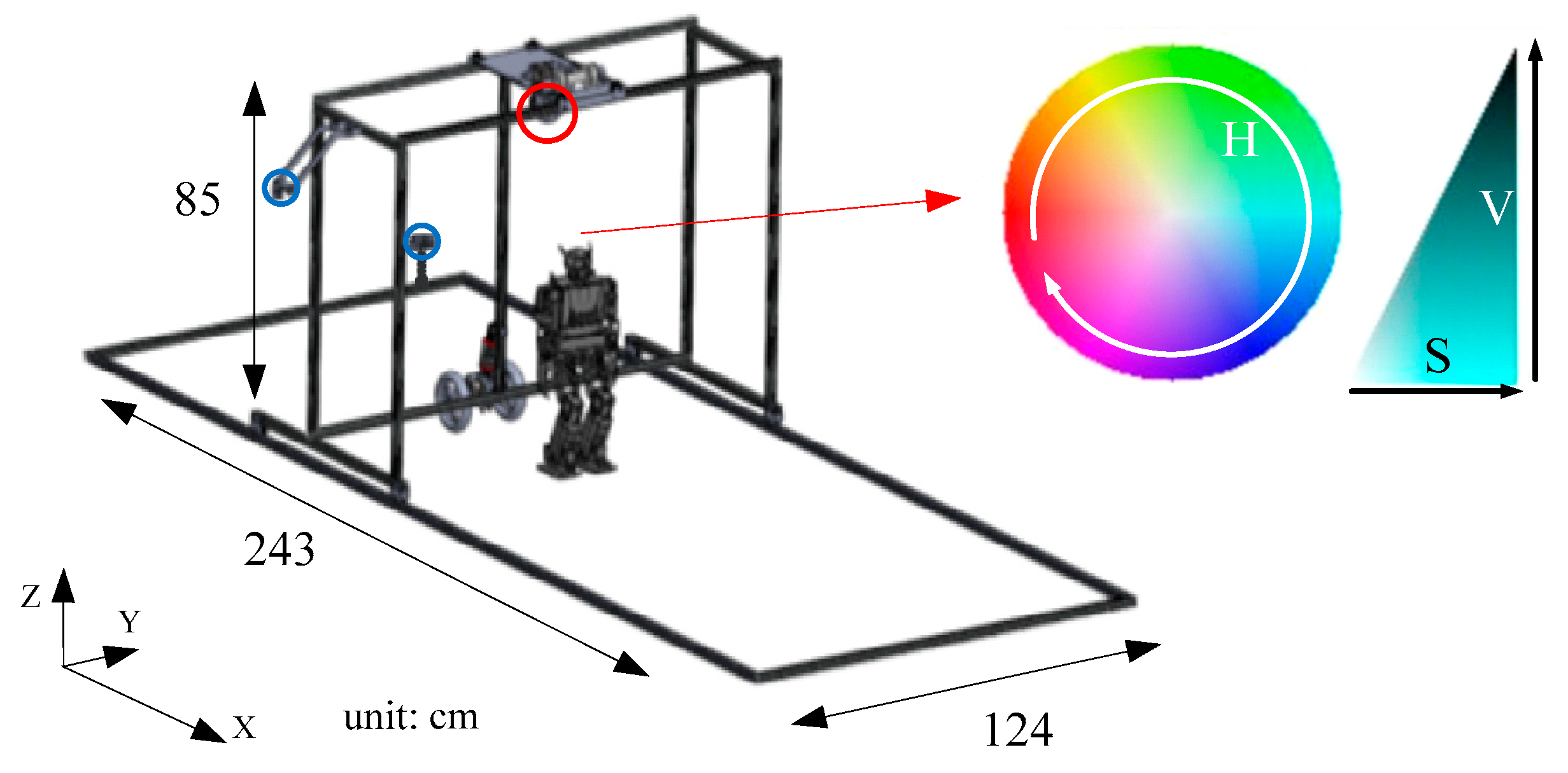
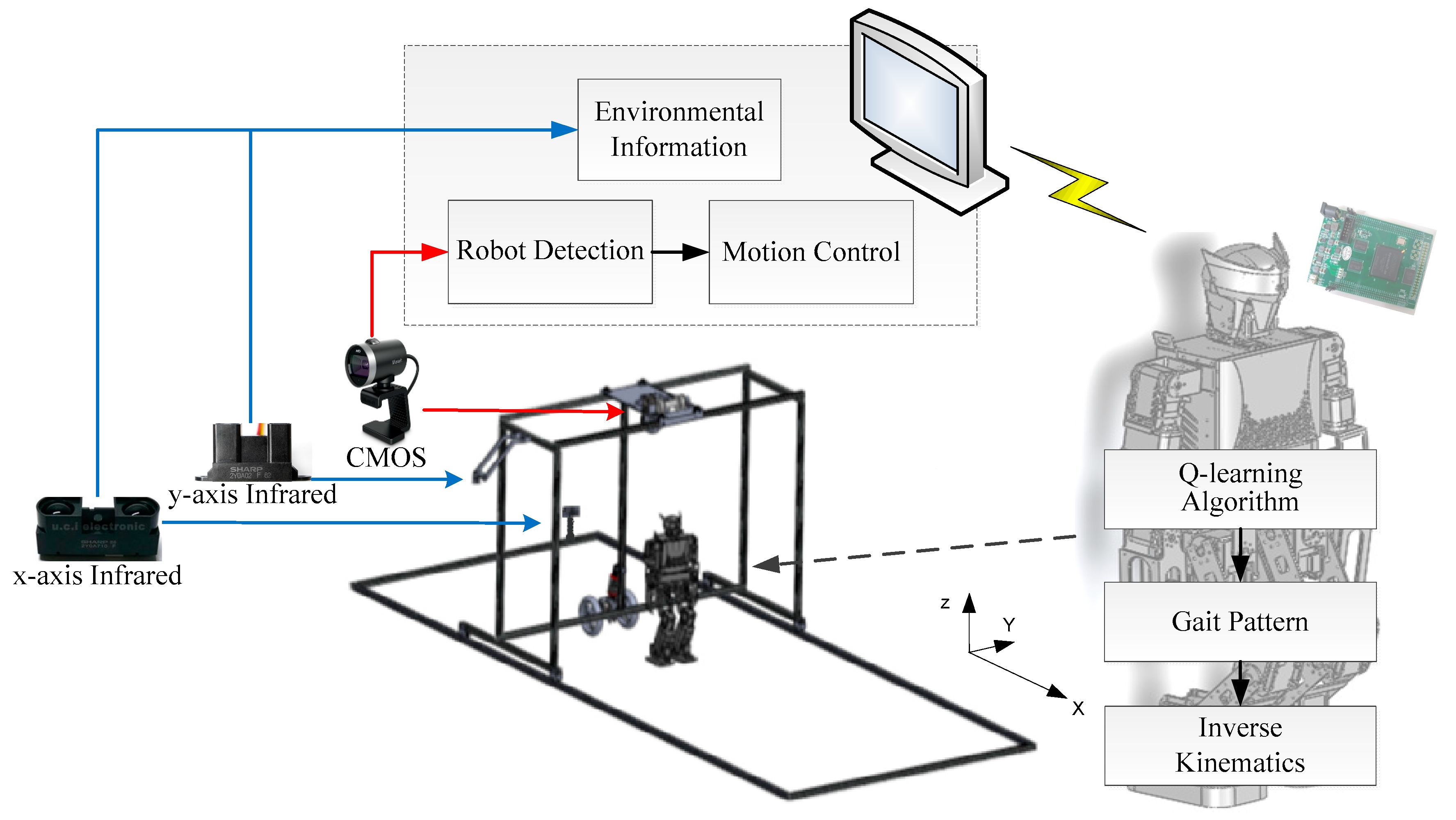
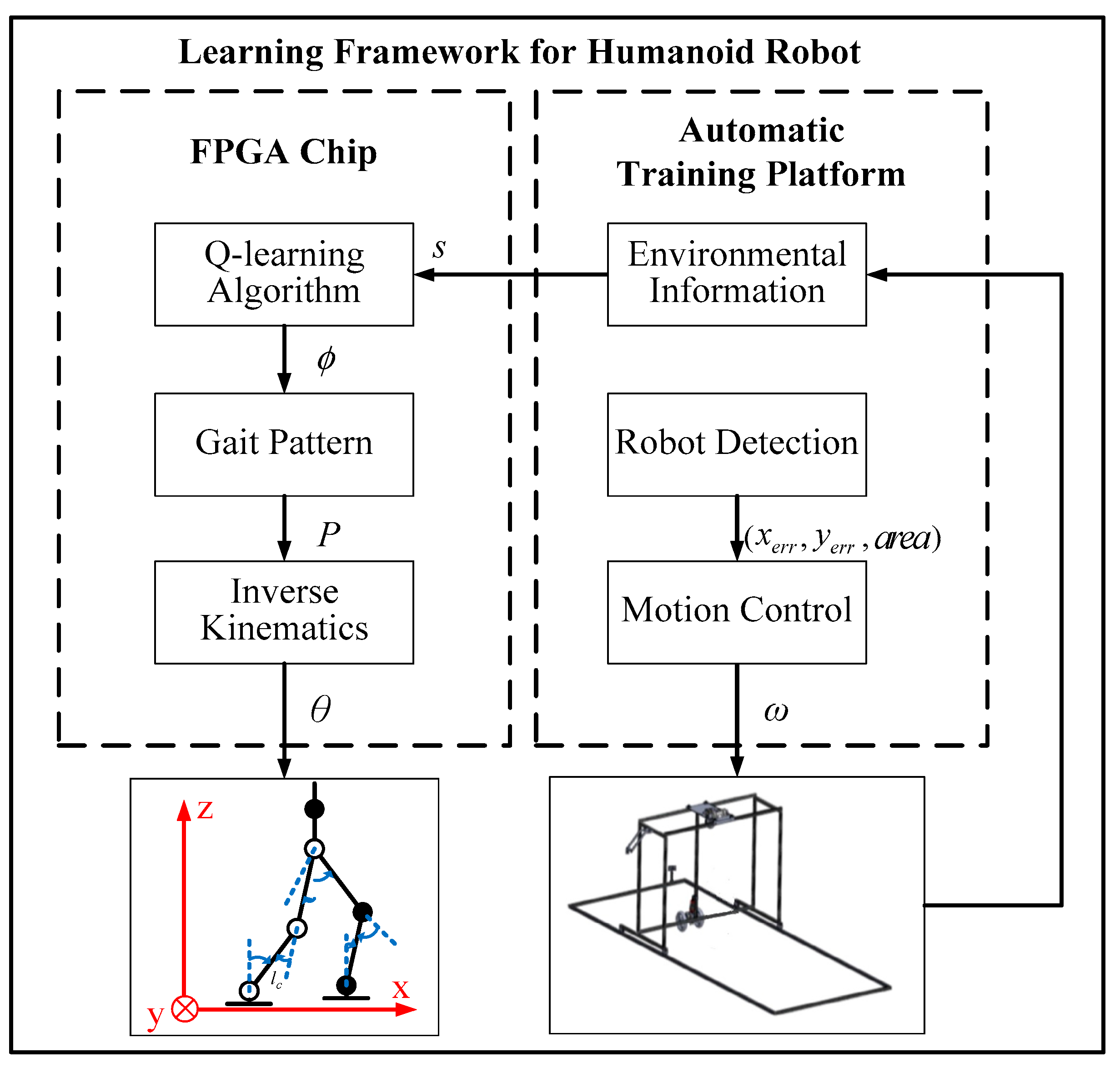
In order to allow the humanoid robot to learn a straightforward gait pattern in the automatic training platform, the proposed learning framework was developed using the system architecture illustrated in Figure 7 and described in Figure 8. The three modules (Q-learning algorithm, gait pattern, and inverse kinematics) were designed and implemented in the FPGA chip to speed up the learning process and to produce real-time bipedal locomotion. In addition, three additional modules (environmental information, robot detection, and motion control) were designed and implemented in the automatic training platform to assist and supervise the humanoid robot in the automatic learning process. Their functions are described below.

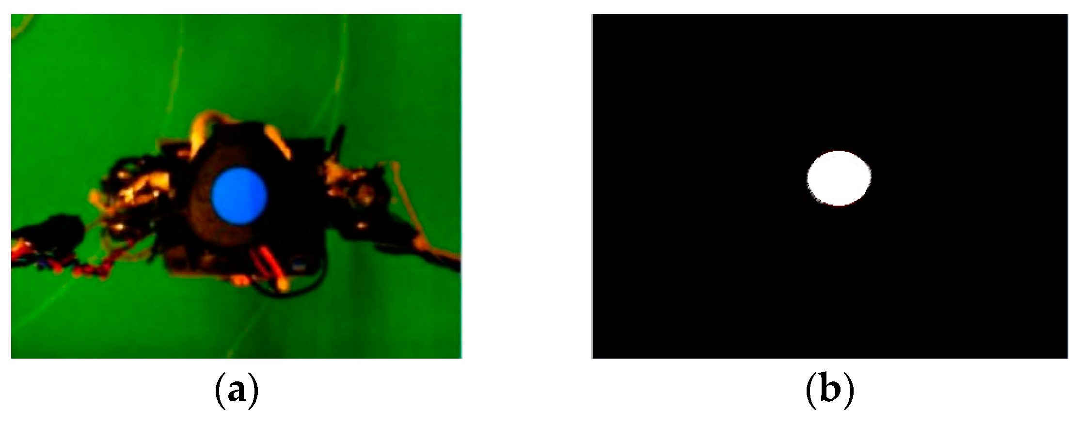
Firstly, the robot’s mark was placed above it to be detected by the CMOS sensor. Pixel errors in the x-axis and y-axis and the area of ​​the robot’s mark $(x_{err},y_{err},area)$ were obtained to follow the robot using the detection module. Secondly, the velocities $\omega$ were required by the automatic training platform to control the motors and to follow the robot from the motion control module. Thirdly, when the humanoid robot walked with its mechanism error and motor backlash in the real environment, its position in the training field $s$ could be obtained based on the measured data from the environmental information module via the x-axis and y-axis infrared sensors. Fourthly, the turning direction $\varphi$, a parameter of the gait pattern, could be calculated according to $s$ to learn the straightforward gait pattern from the Q-learning algorithm module. Fifthly, the trajectory planning $P$, which depended on the turning direction $\varphi$, could be generated from the gait pattern module. Finally, the angle of each joint $\theta$ was determined from the inverse kinematics module based on $P$ so that the robot could exhibit bipedal locomotion.

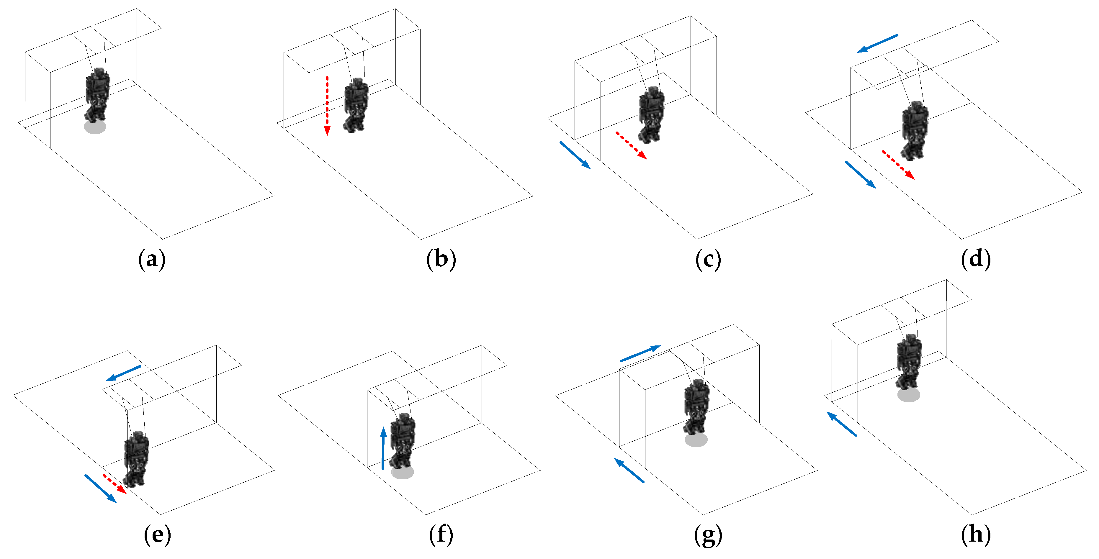
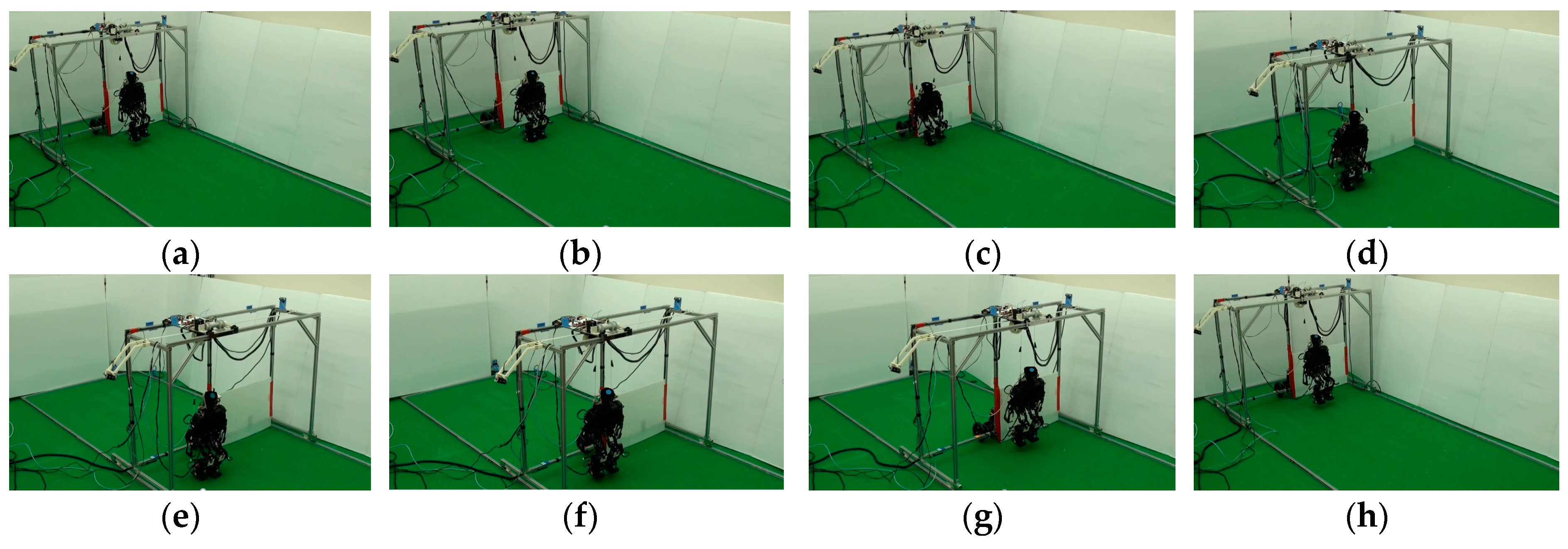
The process of the proposed automatic training platform is described in Figure 9 which consists of several states. In the beginning, the humanoid robot was suspended and then slowly lowered onto the training field, which served as the initial position (the start state), as shown in Figure 9a,b. Next, the straightforward gait pattern was learned while the automatic training platform followed the robot at the same time (the operation state), as shown in Figure 9c,d. Then, once the robot was in danger or once it reached the target region, the humanoid robot was pulled up by the automatic training platform (the end state), as shown in Figure 9e,f. Finally, the automated training platform could return to the initial position and restart the learning process (the return state), as shown in Figure 9g,h.

The procedure of the proposed learning framework based on the automatic training platform can be described as follows:

Step 1:

(Setting State) The robot’s mark is put above the humanoid robot and is detected by a CMOS sensor installed on the automatic training platform.

Step 2:

(Initial State) Pixel errors in the x-axis and y-axis and the area of the robot’s mark $(x_{err},y_{err},area)$ are obtained from the robot detection module tallow the platform to follow the robot.

Step 3:

(Initial State) The velocities $\omega$ are determined from the motion control module to control the motors, allowing the automatic training platform to follow the robot.

Step 4:

(Initial State) The position $s$ of the humanoid robot in the training field is obtained from the environmental information module based on the measured data via the x-axis and y-axis infrared sensors.

Step 5:

(Start State) The humanoid robot is suspended and then slowly placed on the training field, which serves as the initial position.

Step 6:

(Operation State) The turning direction $\varphi$ is calculated from the Q-learning algorithm module based on the position $s$ to learn the straightforward gait pattern.

Step 7:

(Operation State) The trajectory planning $P$, which depends on the turning direction $\varphi$, is generated from the gait pattern module.

Step 8:

(Operation State) The angle of each joint $\theta$ is determined from the inverse kinematics module based on $P$, allowing the robot to exhibit bipedal locomotion.

Step 9:

(End State) When the robot is in danger or when it reaches the target region, the humanoid robot is pulled up by the automatic training platform.

Step 10:

(Return State) The automated training platform returns to Step 5 (Start State) and restarts the learning process.

4. Oscillator-Based Gait Pattern

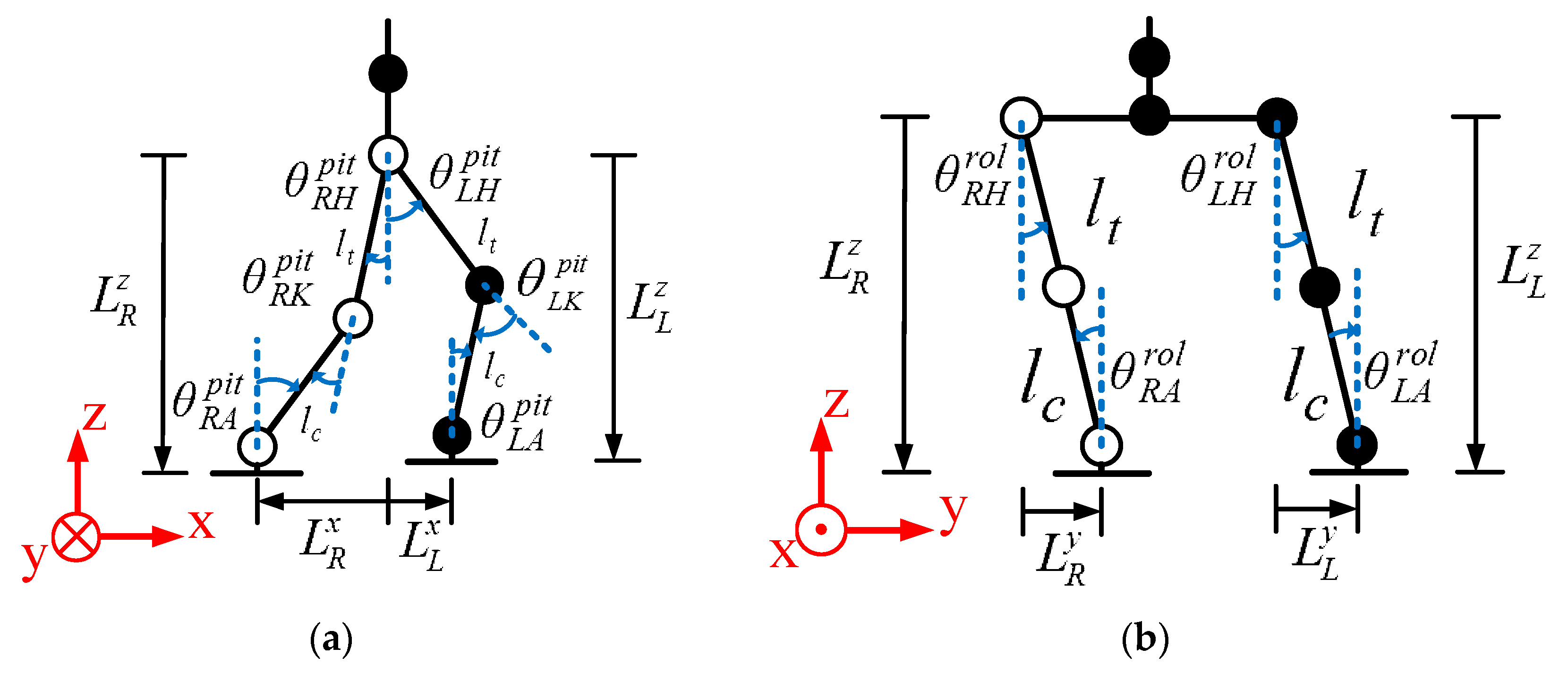
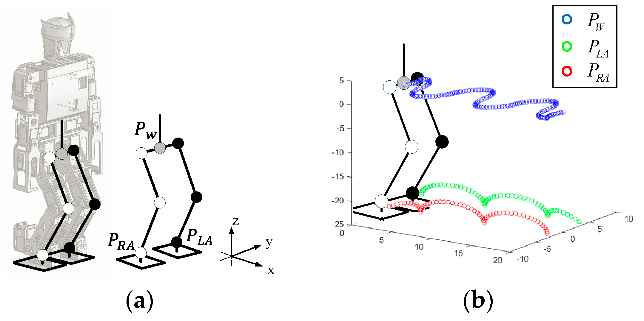
In order to implement a flexible and adaptable gait pattern, oscillators were adopted for the humanoid robot in this paper. Hence, the legs of the humanoid robot and their coordinate system needed to be defined for the gait pattern, as shown in Figure 10a. $P_W=(P_W^x,P_W^y,P_W^z)$ represents the position of the waist, which was considered to be the center of mass (CoM). $P_{RA}=(P_{RA}^x,P_{RA}^y,P_{RA}^z)$ and $P_{LA}=(P_{LA}^x,P_{LA}^y,P_{LA}^z)$ represent the positions of the left and right ankles, respectively. The right and left legs interchanged as the support leg to obtain the walking ability of the humanoid robot. 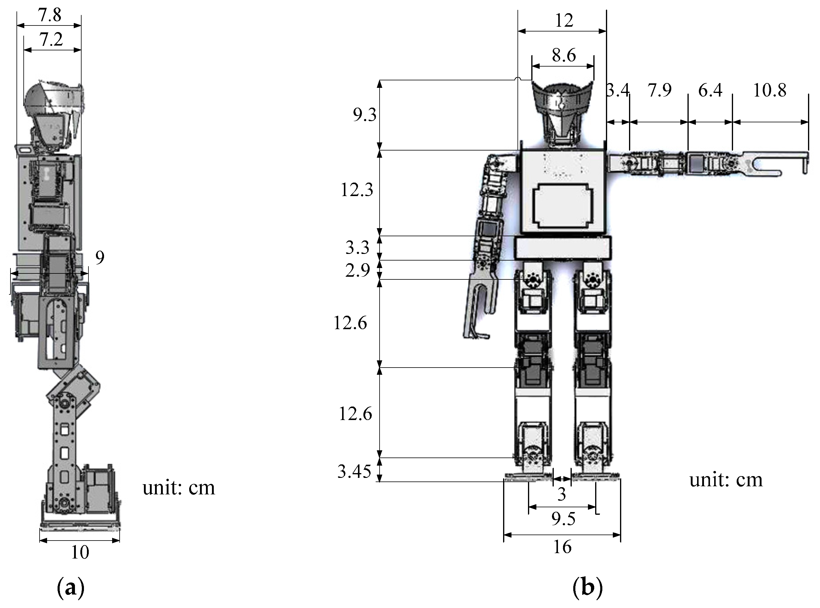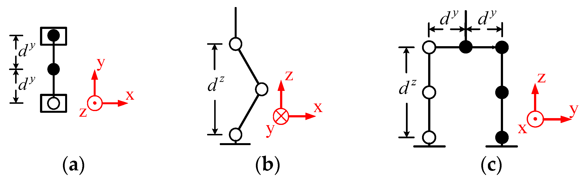Hence, the three-dimensional gait pattern could be described by the position of the waist, and left and right ankles $(P_W,P_{LA},P_{RA})$, as shown in Figure 10b. The standing posture of the robot and its leg parameters are shown in Figure 11, where $d^y$ is the distance between the waist $P_W$ and the hip, and $d^z$ is the distance between the hip and the ankle.

The humanoid robot was a high-dimensional complex structure; thus, three-dimensional trajectory planning $P=(P_W,P_{LA},P_{RA})$ was generated by the oscillators based on the Cartesian coordinate system to simplify the gait pattern of the humanoid robot. The oscillators could be divided into a balance oscillator and two movement oscillators, located at the CoM $P_W$, and left and right ankles $(P_{LA},P_{RA})$, respectively, to generate the trajectories. The purpose of the balance oscillator was to maintain the balance of the robot and to generate the CoM trajectory. The purpose of the movement oscillators was to support and move the body of the robot and to generate the left and right ankle trajectories. Since the gait pattern was a periodic behavior, a sinusoidal function was adopted for the oscillators, which was adjusted by the walking phase $p$ to simplify the design method. The equations of the oscillators at the CoM $P_W$, and left and right ankles $(P_{LA},P_{RA})$ can be expressed as follows:

$$\begin{array}{ll}{P}_W& =os{c}_W+P_W^o\\ & =(os{c}_W^x(p),os{c}_W^y(p),os{c}_W^z(p))+(P_W^{x0},P_W^{y0},P_W^{z0})\\ & =({\rho }_W^x(p)\sin ({\omega }_W^x(p)t+{\delta }_W^x(p)),{\rho }_W^y(p)\sin ({\omega }_W^y(p)t+{\delta }_W^y(p)),\\ & \hspace{1em}{\rho }_W^z(p)\sin ({\omega }_W^z(p)t+{\delta }_W^z(p)))+(0,0,0),\hspace{1em}p\in \{1,2,\cdots ,6\}\end{array},$$

(14)

$$\begin{array}{ll}{P}_{LA}& =os{c}_{LA}+P_{LA}^o\\ & =(os{c}_{LA}^x(p),os{c}_{LA}^y(p),os{c}_{LA}^z(p),os{c}_{LA}^{\varphi }(p))+(P_{LA}^{x0},P_{LA}^{y0},P_{LA}^{z0},P_{LA}^{\varphi 0})\\ & =({\rho }_{LA}^x(p)\sin ({\omega }_{LA}^x(p)t+{\delta }_{LA}^x(p)),{\rho }_{LA}^y(p)\sin ({\omega }_{LA}^y(p)t+{\delta }_{LA}^y(p)),\\ & \hspace{1em}{\rho }_{LA}^z(p)\sin ({\omega }_{LA}^z(p)t+{\delta }_{LA}^z(p)),{\rho }_{LA}^{\varphi }(p)\sin ({\omega }_{LA}^{\varphi }(p)t+{\delta }_{LA}^{\varphi }(p)))+(0,d^y,-d^z,0),\hspace{1em}p\in \{1,2,\cdots ,6\}\end{array},$$

(15)

and

$$\begin{array}{ll}{P}_{RA}& =os{c}_{RA}+P_{RA}^o\\ & =(os{c}_{RA}^x(p),os{c}_{RA}^y(p),os{c}_{RA}^z(p),os{c}_{RA}^{\varphi }(p))+(P_{RA}^{x0},P_{RA}^{y0},P_{RA}^{z0},P_{RA}^{\varphi 0})\\ & =({\rho }_{RA}^x(p)\sin ({\omega }_{RA}^x(p)t+{\delta }_{RA}^x(p)),{\rho }_{RA}^y(p)\sin ({\omega }_{RA}^y(p)t+{\delta }_{RA}^y(p)),\\ & \hspace{1em}{\rho }_{RA}^z(p)\sin ({\omega }_{RA}^z(p)t+{\delta }_{RA}^z(p)),{\rho }_{RA}^{\varphi }(p)\sin ({\omega }_{RA}^{\varphi }(p)t+{\delta }_{RA}^{\varphi }(p)))+(0,-d^y,-d^z,0),\hspace{1em}p\in \{1,2,\cdots ,6\}\end{array},$$

(16)

where $os{c}_W$, $os{c}_{LA}$, and $os{c}_{RA}$ are the oscillators at the CoM, and left and right ankles, respectively, $p_W^0$, $p_{RA}^0$, and $p_{LA}^0$ are the starting points of the CoM, and left and right ankles, respectively, and ($\rho$,$\omega$,$\delta$) are the amplitude, angular velocity, and phase shift of the oscillator parameters. All oscillators involved three axes of the sub-oscillator (x-axis, y-axis, and z-axis) in three-dimensional space, and the two movement oscillators additionally included one sub-oscillator for the turning direction $\varphi$.

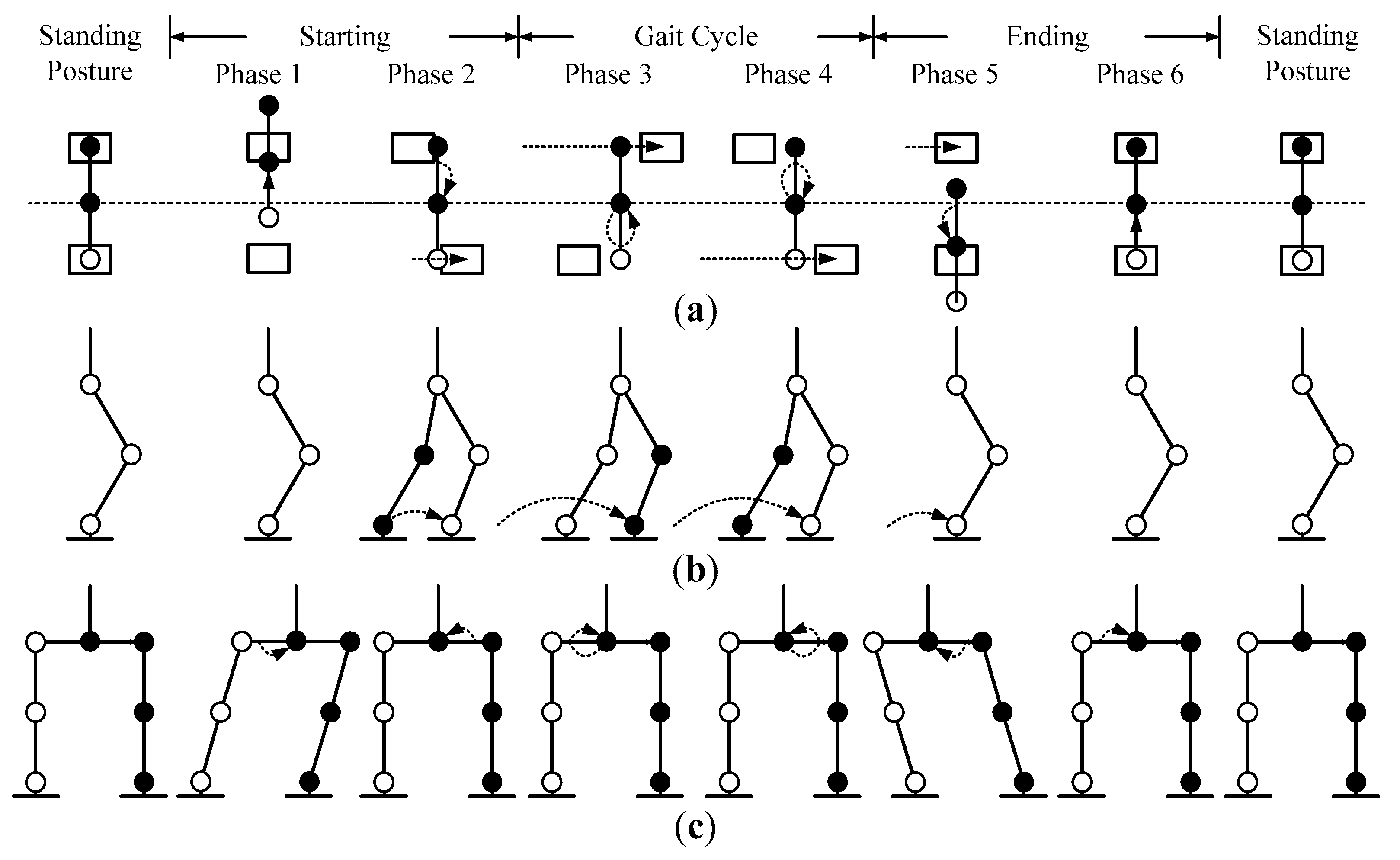
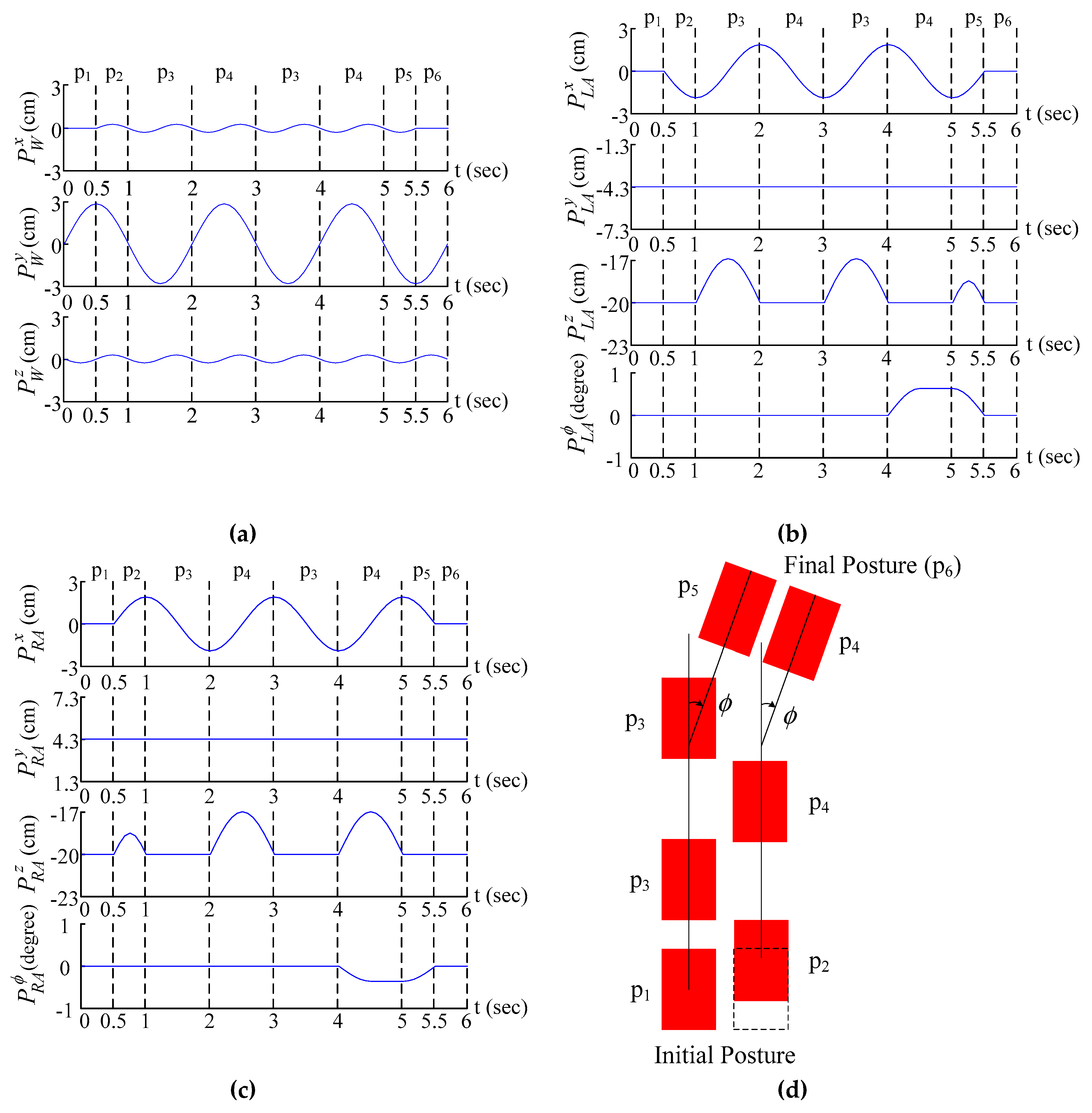
The gait pattern could be described as three modes: starting mode, gait cycle mode, and ending mode, and each mode was divided into two phases. Hence, a complete walking process consisted of six phases: Phase 1–6 ($p1$–$p6$) [7], as shown in Figure 12. The leftmost (initial posture) and the rightmost (final posture) postures were both standing postures. In these six phases, the parameters of the CoM in terms of the x-axis, y-axis, and z-axis (S_Wx, S_Wy, H_W) were the same as those involved in the walking process. Phase 1 ($p1$) and Phase 2 ($p2$) were classified as the starting mode, which only worked once at the beginning of the walking process. The CoM swung from the middle to the left, and both feet remained on the floor in Phase 1. The CoM swung from the left back to the middle, with the left foot still on the floor, and the right foot lifted a height $H_R^S$ to move one step forward $S_R^S$ in Phase 2. Phase 3 ($p3$) and Phase 4 ($p4$) were classified as the gait cycle mode, which worked repeatedly in the middle of the walking process. The CoM swung in a circular motion on the right side, with the right foot on the floor, and the left foot lifted a height $H_L^G$ to move one stride forward $S_L^G$ in Phase 3. The CoM swung in a circular motion on the left side, with the left foot on the floor, and the right foot lifted a height $H_R^G$ to move one stride forward $S_R^G$ in Phase 4. Phase 5 ($p5$) and Phase 6 ($p6$) were classified as the ending mode, which also only worked once at the end of the walking process. The CoM swung to the right side, with the right foot on the floor, and the left foot lifted a height $H_L^E$ to move one step forward $S_L^E$ in Phase 5. The CoM swung from the right back to the middle, with both feet on the floor, in Phase 6.

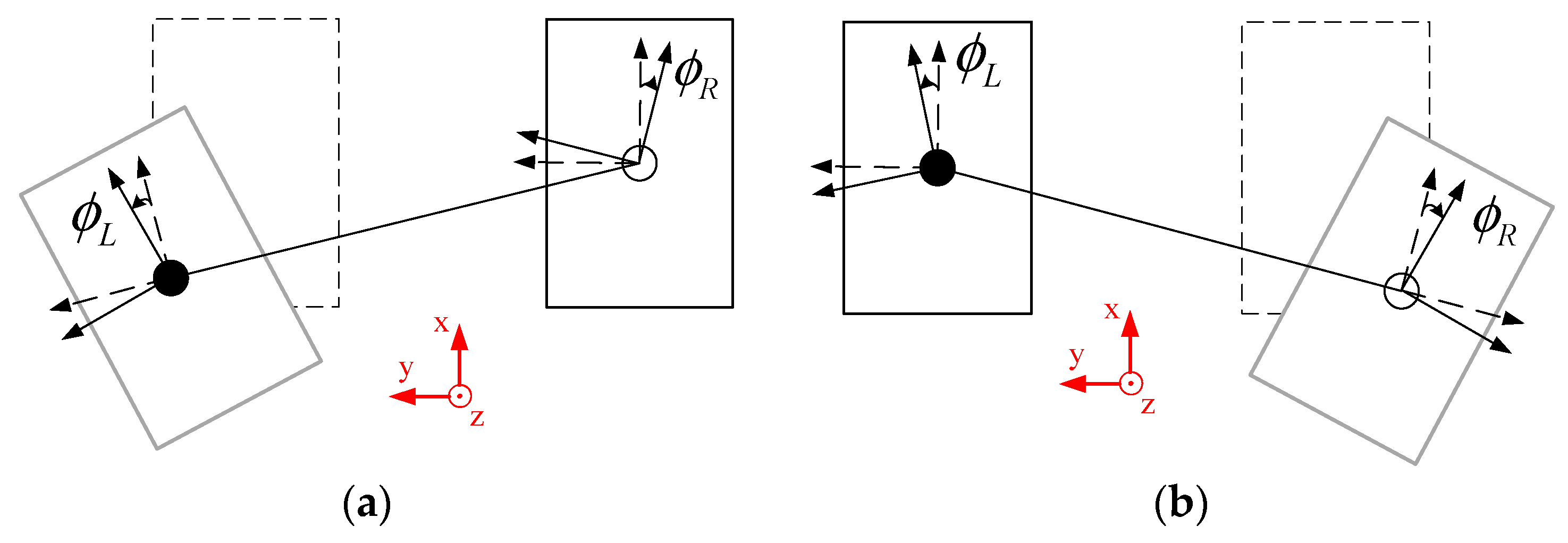
The turning direction $\varphi$ was also involved in the designed gait pattern to increase the flexibility of the humanoid robot. When humans change direction, it is natural for them to rotate their legs. Hence, the movement oscillators were related to the turning direction of the humanoid robot to generate the trajectories. The turning direction of the humanoid robot is shown in Figure 13 and it could also be assigned a starting mode, gait cycle mode, and ending mode, which in total contained six phases ($p1$–$p6$). If the left foot moved forward and the right foot was on the floor in the complete walking process, the turning left direction could be executed as shown Figure 13a. Similarly, if the right foot moved forward and the left foot was on the floor in the complete walking process, the turning right direction could be executed as shown Figure 13b. The turning direction was distributed to both feet, the moving foot and the foot on the floor, to rotate the legs (${\varphi }_L$, ${\varphi }_R$) in a ratio of three to seven. In the turning left direction, it is expressed by

$$({\varphi }_L,{\varphi }_R)=(0.3\ast \varphi ,-0.7\ast \varphi ).$$

(17)

In the turning right direction, it is expressed by

$$({\varphi }_L,{\varphi }_R)=(-0.7\ast \varphi ,0.3\ast \varphi ).$$

(18)

In this way, the designated region could be effectively reached using the turning direction. The parameter set of the oscillator-based gait pattern with the period of a walking step T in the walking process is shown in

Table 3. Parameter set of the oscillator-based gait pattern in a walking process.

Parameter	Starting mode		Gait cycle mode		Ending mode
	Phase 1	Phase 2	Phase 3	Phase 4	Phase 5	Phase 6
$({\rho }_W^x(p),{\rho }_W^y(p),{\rho }_W^z(p))$	(0, SWy, HW)	(SWx, SWy, HW)	(SWx, SWy, HW)	(SWx, SWy, HW)	(SWx, SWy, HW)	(0, SWy, HW)
$({\omega }_W^x(p),{\omega }_W^y(p),{\omega }_W^z(p))$	(2π/T, π/T, 2π/T)		(2π/T, π/T, 2π/T)		(2π/T, π/T, 2π/T)
$({\delta }_W^x(p),{\delta }_W^y(p),{\delta }_W^z(p))$	(0, 0, π)	(0, π/2, 0)	(π, π, π)	(π, 0, π)	(π, π, π)	(0, 0, 0)
$({\rho }_{LA}^x(p),{\rho }_{LA}^y(p),{\rho }_{LA}^z(p),{\rho }_{LA}^{\varphi }(p))$	(0, 0, 0, 0)	($S_R^S$/2, 0, 0,${\varphi }_L$)	($S_L^G$/4, 0,$H_L^G$,${\varphi }_L$)	($S_R^G$/4, 0, 0,${\varphi }_L$)	($S_L^E$/2, 0,$H_L^E$,${\varphi }_L$)	(0, 0, 0, 0)
$({\omega }_{LA}^x(p),{\omega }_{LA}^y(p),{\omega }_{LA}^z(p),{\omega }_{LA}^{\varphi }(p))$	(π/T, 0, 2π/T, 0)		(π/T, 0, π/T, π/T)		(π/T, 0, 2π/T, π/T)
$({\delta }_{LA}^x(p),{\delta }_{LA}^y(p),{\delta }_{LA}^z(p),{\delta }_{LA}^{\varphi }(p))$	(0, 0, 0, 0)	(π, 0, 0, 0)	(3π/2, 0, 0, 0)	(π/2, 0, 0, 0)	(3π/2, 0, 0, π/2)	(0, 0, 0, 0)
$({\rho }_{RA}^x(p),{\rho }_{RA}^y(p),{\rho }_{RA}^z(p),{\rho }_{RA}^{\varphi }(p))$	(0, 0, 0, 0)	($S_R^S$/2, 0,$H_R^S$,${\varphi }_R$)	($S_L^G$/4, 0,${\varphi }_R$)	($S_R^G$/4, 0,$H_R^G$,${\varphi }_R$)	($S_L^E$/2, 0,${\varphi }_R$)	(0, 0, 0, 0)
$({\omega }_{RA}^x(p),{\omega }_{RA}^y(p),{\omega }_{RA}^z(p),{\omega }_{RA}^{\varphi }(p))$	(π/T, 0, 2π/T, 0, 0)		(π/T, 0, π/T, π/T, π/T)		(π/T, 0, 2π/T, π/T, π/T)
$({\delta }_{RA}^x(p),{\delta }_{RA}^y(p),{\delta }_{RA}^z(p),{\delta }_{RA}^{\varphi }(p))$	(0, 0, 0, 0)	(0, 0, 0, 0)	(π/2, 0, 0, 0)	(3π/2, 0, 0, 0)	(π/2, 0, 0, π/2)	(0, 0, 0, 0)

. Trajectories and footprints with turning direction are shown in Figure 14.

5. Learning the Straightforward Gait Pattern

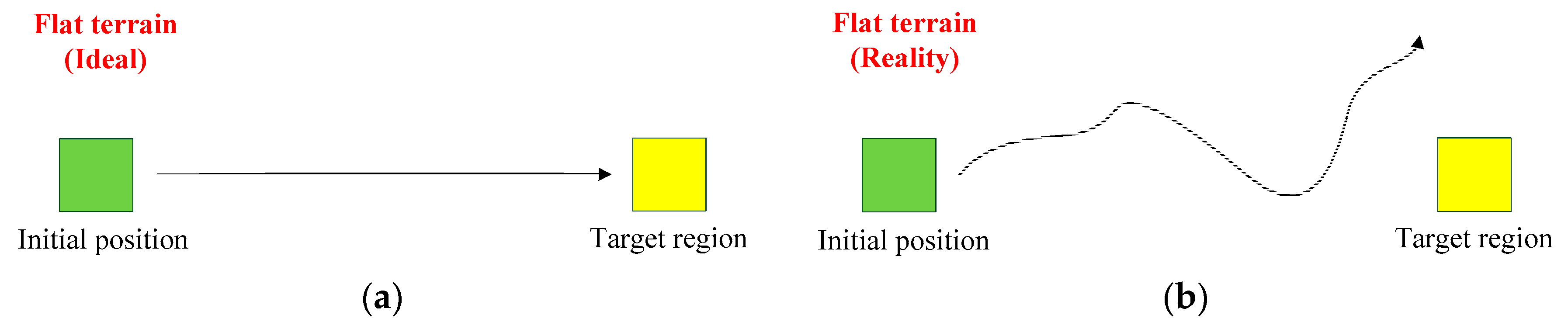
In this paper, a flat terrain was adopted for the humanoid robot to learn the straightforward gait pattern. Most gait patterns are designed assuming an ideal situation, where the mechanism and motors are working well. However, the long-term operation of the humanoid robot may result in mechanism error and motor backlash. Moreover, the real environment also cause the humanoid robot to exhibit some unexpected behaviors. As shown in Figure 15, the target region (yellow area) was placed in front of the robot and the robot started from the initial position (green area). In an ideal situation, the humanoid robot could walk straight to reach the target region, as shown in Figure 15a. In a realistic situation, the humanoid robot could not walk straight and could not reach the target region, as shown in Figure 15b. Hence, the Q-learning algorithm was adopted to adjust the turning direction $\varphi$, allowing the robot to walk straight to reach the target region from the initial position according to the environmental information.

The Q-learning algorithm is a well-known model-free reinforcement learning method, and it employs the concept of the Markov decision process (MDP) with finite state and action [15,22]. An optimal policy can be learned by using Q-learning to maximize the expected reward [14]. During the learning process, an action is taken by an agent and interacts with the environment for one state to another state. After taking an action $a$ for state $s$, the policy can be updated through an action-value function $Q(s,a)$. A Q-table is composed of Q-values which are designed and evaluated by the action-value function $Q(s,a)$ for the agent. The Q-values with state $s$ and action $a$ are updated as follows [12,14,16]:

$$Q(s,a)=Q(s,a)+\alpha \left[r+\gamma \begin{array}{c}\\ \max \\ a^{\prime }\end{array}Q(s^{\prime },a^{\prime })-Q(s,a)\right],$$

(19)

where $\alpha$ and $\gamma$ are the learning rate and discount factor, respectively, $r$ is the reward, which can be evaluated after taking action $a$ for state $s$, $s^{\prime }$ is the next state after taking action $a$ for state $s$, and $\max Q(s^{\prime },a^{\prime })$ denotes the maximum future Q-value, while $\epsilon$-greedy is set to choose a random action. The pseudo-code of the Q-learning algorithm is shown in

Table 4. Pseudo-code of the Q-learning algorithm.

Algorithm: Q-learning Algorithm.

Initialize$Q(s,a)$ arbitrarily

Repeat (for each episode):

Initialize $s$

Repeat (for each step of episode):

Choose $a$ from $s$ using policy derived from $Q$(e.g., $\epsilon$-greedy)

Take action $a$, observe $r$, $s^{\prime }$

$Q(s,a)\leftarrow Q(s,a)+\alpha \left[r+\gamma \begin{array}{c}\\ \max \\ a^{\prime }\end{array}Q(s^{\prime },a^{\prime })-Q(s,a)\right]$

$s\leftarrow s^{\prime }$

Until $s$ is terminal

.

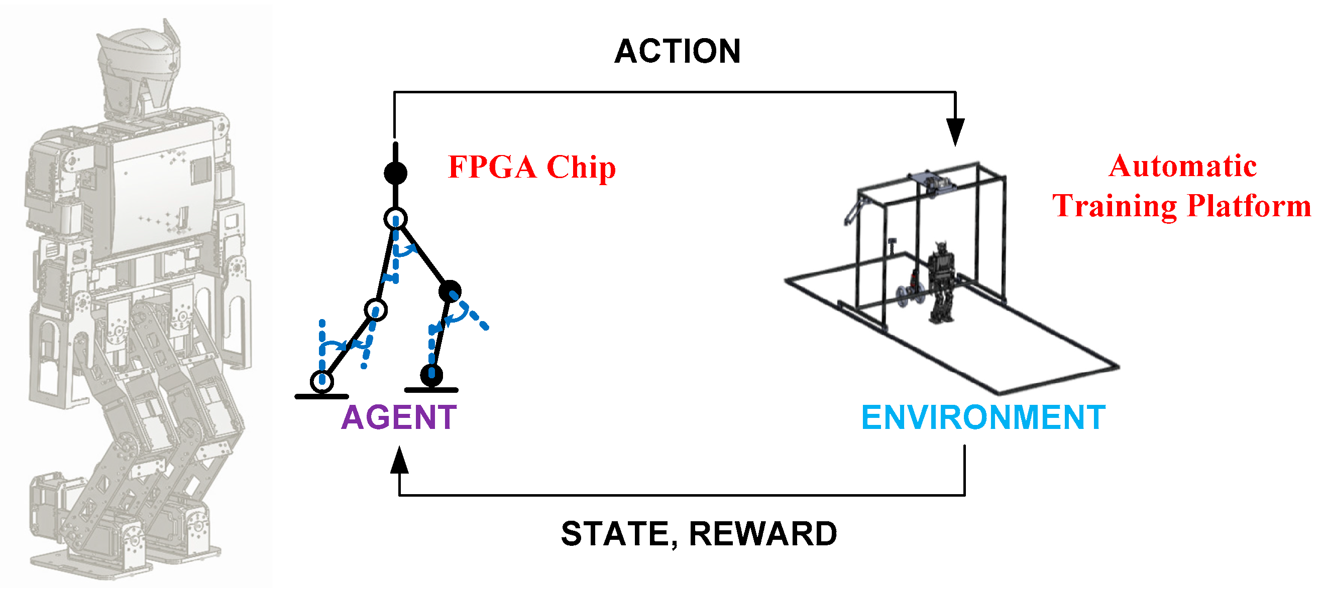
The proposed learning framework with the Q-learning algorithm is shown in Figure 16. The FPGA chip allowed the agent to learn the straightforward gait pattern, and the automatic training platform worked to follow and train the robot. In order to adjust the turning direction $\varphi$ using the Q-learning algorithm, three elements of the Q-learning algorithm were defined and designed to update the Q-values of the Q-table: (1) state ($s$), the environmental information measured by the infrared sensors installed on the automatic training platform to offer the position of the humanoid robot in the training field; (2) action ($a$), the turning direction $\varphi$ selected according to state $s$ for the gait pattern of the humanoid robot; (3) reward ($r$), the learning guideline dependent on state $s$ and action $a$ to strengthen or weaken the selected action.

5.1. State for the Straightforward Gait Pattern

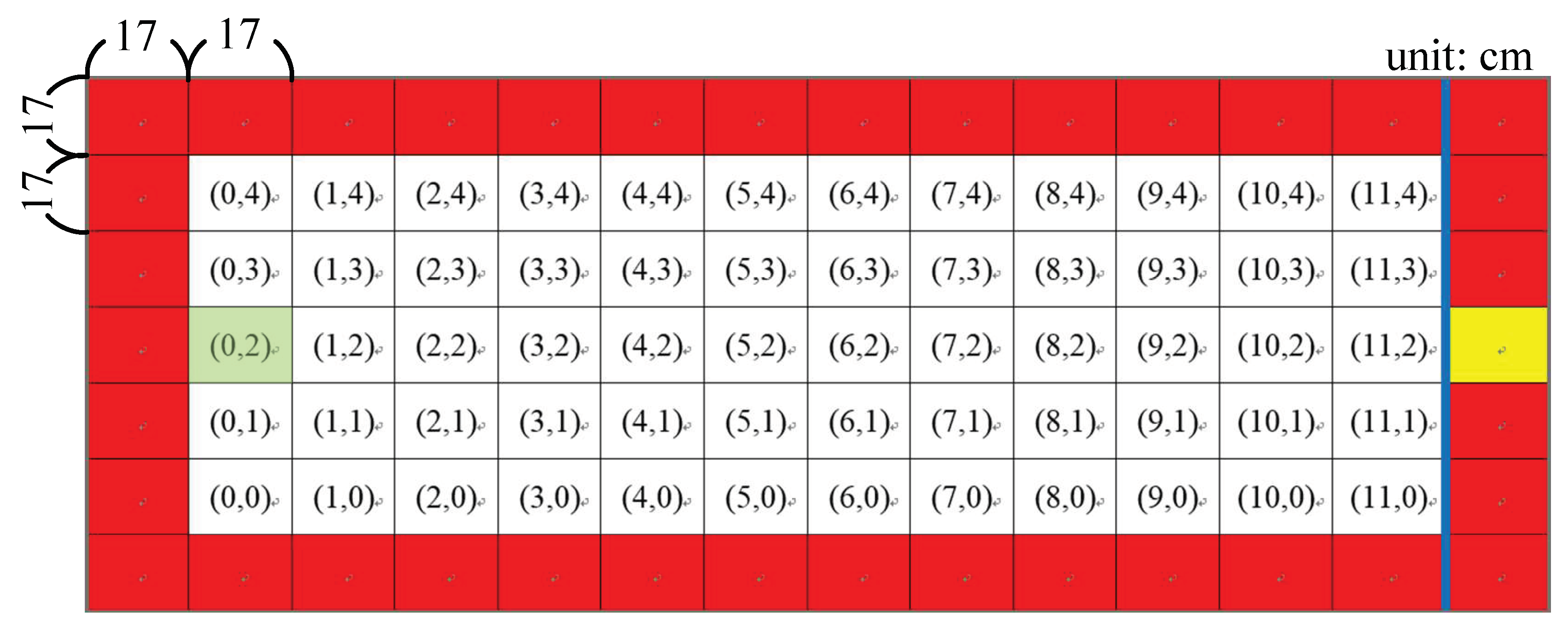
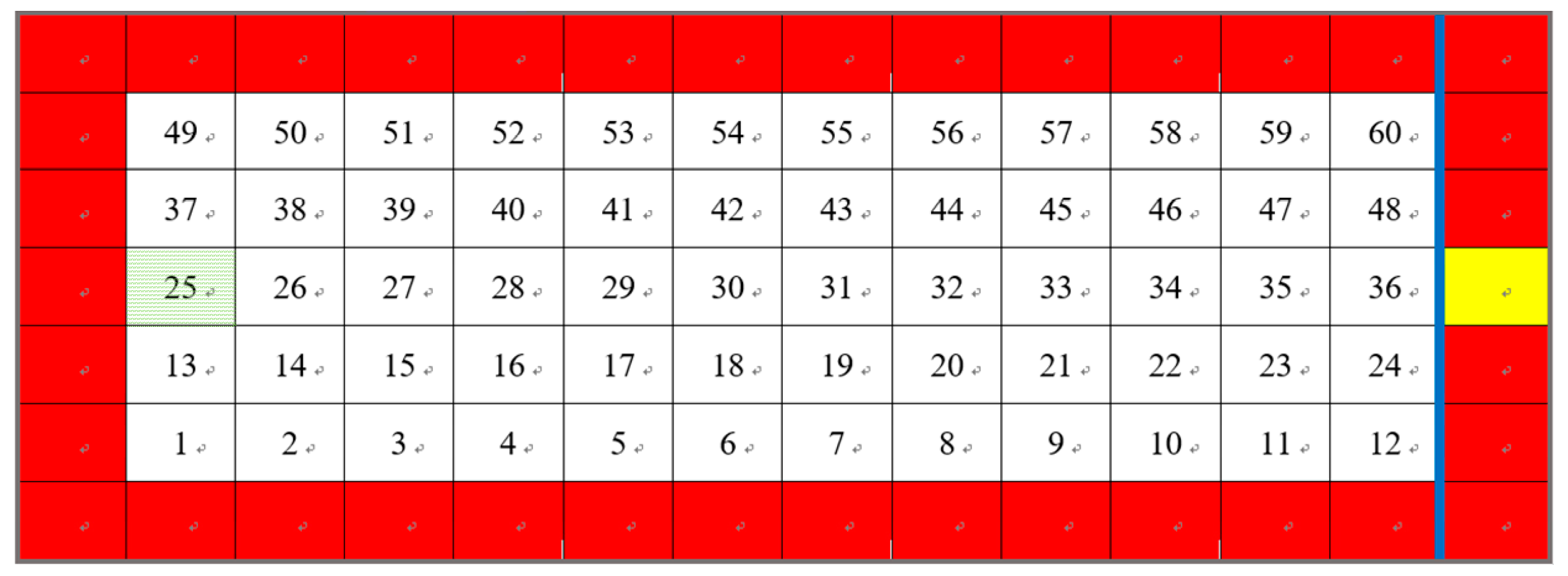
In the learning process, the automatic training platform was adopted not only for supervision to protect the humanoid robot, but also to obtain the current environmental information of state $s$ required by the Q-learning algorithm. As shown in Figure 17, there were 60 total states of the coordinate system in the training field. The green area denotes the initial position, i.e., the start point of the robot. The yellow region denotes the target region that needs to be reached from the initial position after passing the blue line, which denotes the target distance. Similarly, the red color denotes the danger regions or the boundary of the automatic training platform which the robot cannot reach. These 60 states can be used to present the current position of the robot in the training field. The states can be obtained as follows:

$$s=12*d_y+d_x+1,$$

(20)

where $d_x$ and $d_y$ are the x-axis and y-axis distances of the robot in the training field measured using the two infrared sensors.

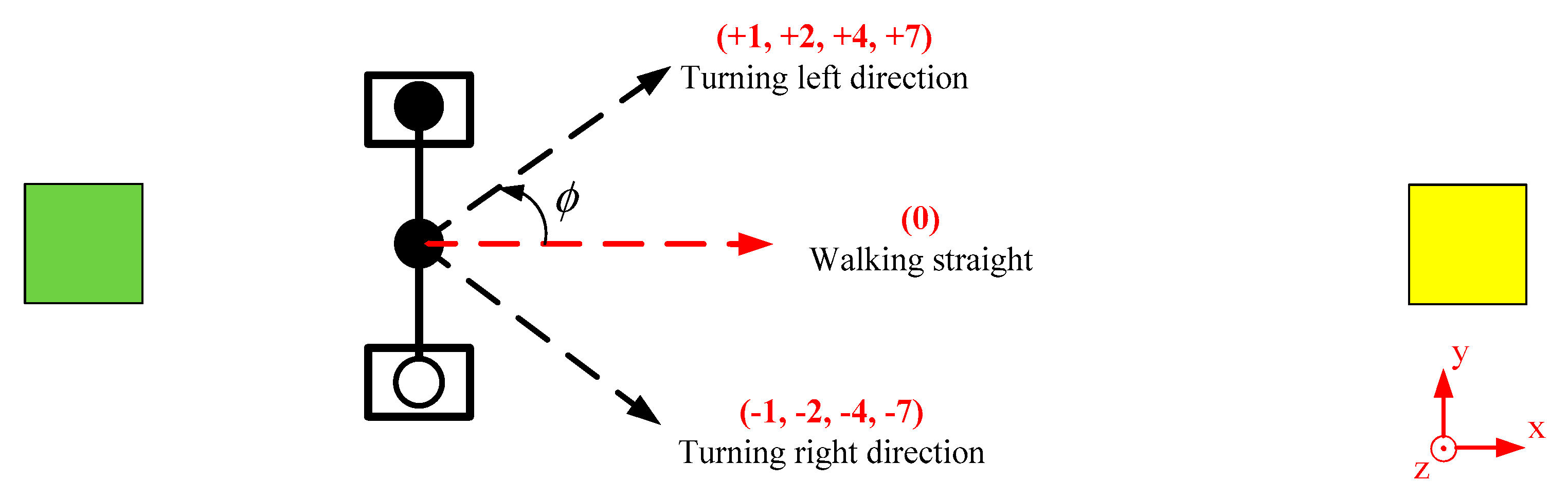
5.2. Action for the Straightforward Gait Pattern

In order to reach the target region from the initial position, the turning direction $\varphi$ of the humanoid robot was designated as action $a$ by the Q-learning algorithm. There were a total of 9 actions that could be selected, as shown in

Table 5. Actions of the Q-learning algorithm.

Type	Actions
$\varphi$(degree))	−7	−4	−1	−2	0	+1	+2	+4	+7

. Instead of the value 0, four levels labeled minor (value 1), middle (value 2), major (value 4), and urgent (value 7) were designed to allow the robot to walk straight to the target region. These four levels included positive (+) and negative (−) values to realize the turning left direction and turning right direction for the robot, as shown in Figure 18, while the value 0 represented walking straight. However, only one action $a$ could be selected based on the obtained state $s$ to estimate an appropriate policy in the training field.

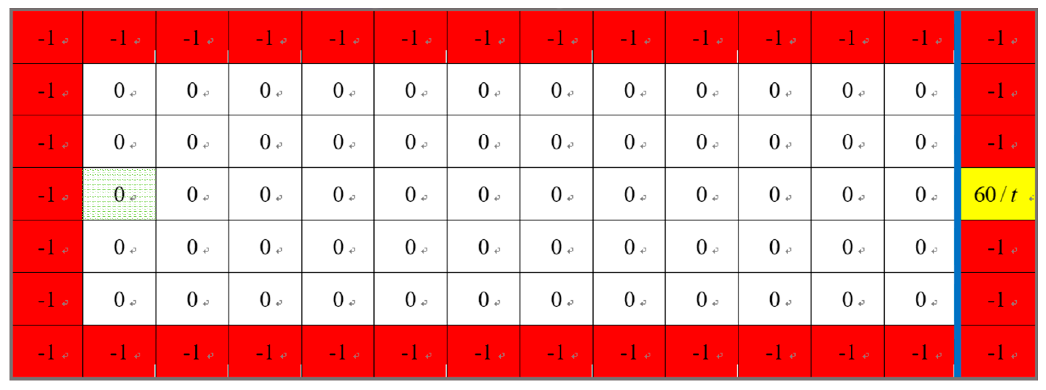
5.3. Reward for the Straightforward Gait Gattern

In the learning process, after a selected action $a$ is taken by an agent and interacts with the environment, a reward $r$ can be returned to the agent. The learning guideline offered a reward to implement the straightforward gait pattern. If a good reward was returned, the selected action was strengthened. Similarly, if a bad reward was returned, the selected action was weakened. Hence, the reward was used to update the policy. The positive and negative rewards were respectively designated in the target region and danger region. In this way, the humanoid robot was attracted or repelled to achieve the straightforward gait pattern. In addition, the time of one learning process $t$ was involved in the reward for the humanoid robot to walk approximately in a straight line and reach the target region, as shown in Figure 19. The reward can be established as follows:

$$r=\{\begin{array}{cc}60/t,& ifachievetargetregion\\ 0,& otherwise\\ -1,& ifachievedangerregion\end{array},$$

(21)

where $t$ is the time of one learning process and it is greater than 0.

6. Experimental Results

The performance of the proposed learning framework is illustrated in this section. The straightforward gait pattern was learned for the humanoid robot using an FPGA chip and an automatic training platform in a training field. The real learning process of the proposed learning framework is demonstrated with four states in Figure 20. In the start state, the humanoid robot was suspended and then slowly lowered by the automatic training platform in the initial position, as shown in Figure 20a,b. In the operation state, the humanoid robot was followed by the automatic training platform when walking from the initial position to the front coordinate of the training field, as shown in Figure 20c,d. In the end state, the humanoid robot reached the end position and then was pulled up by the automatic training platform, as shown in Figure 20e,f. In the return state, the humanoid robot was returned by the automatic training platform to the initial position, as shown in Figure 20g,h. The turning direction was adjusted by the Q-learning algorithm and the walking path of the humanoid robot could also be recorded in this learning process.

Based on the proposed learning framework, there were a total of 594 episodes executed to learn the straightforward gait pattern for the humanoid robot. The target region, with a center of 229.5 cm, 59.5 cm, was located in front of the initial position (25.5 cm, 59.5 cm) where the humanoid robot began walking in each episode. The target distance was where the x-coordinate of the training field was 221 cm. In the learning process, an episode was terminated when the humanoid robot reached the danger region or the target region. The Q-table could be updated by selecting the turning direction according to the position of the robot in the training field. The walking paths of the humanoid robot in these 594 episodes were recorded to analyze the learning process, and they could be divided into three stages: (1) initial stage, (2) middle stage, and (3) final stage, as shown in Figure 21, Figure 22 and Figure 23.

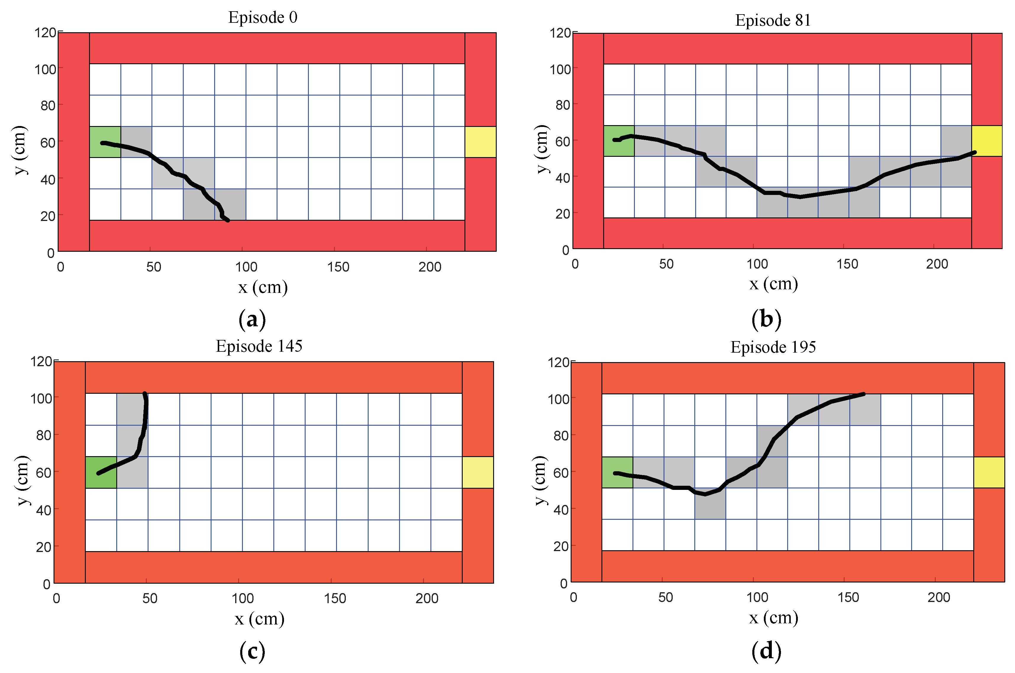
6.1. Initial Stage of the Learning Process

Episodes 0 to 200 represented the initial stage of the learning process, as shown in Figure 21. Episode 0 shows that the humanoid robot could only walk in a straight line to approximately half of the target distance, as shown in Figure 21a. After a few learning processes, episode 81 shows that the humanoid robot could reach the target region, as shown in Figure 21b. However, most episodes in the initial stage, such as episodes 145 and 195, show that the humanoid robot still could not reach the target distance, as shown in Figure 21c,d.

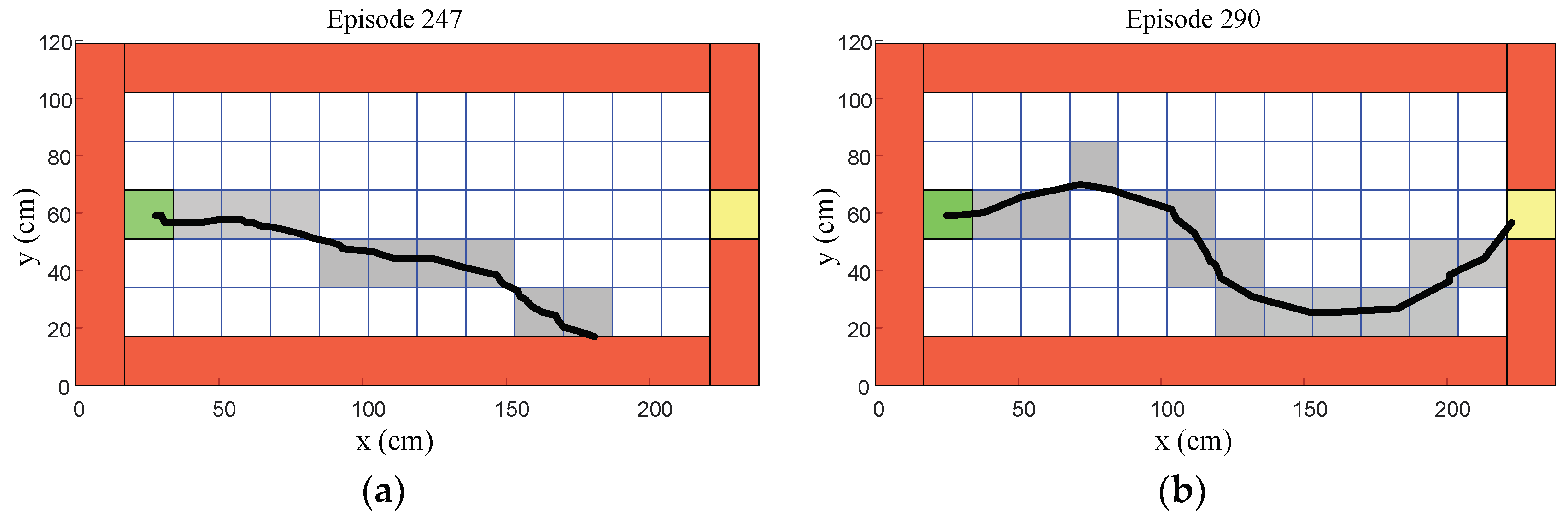
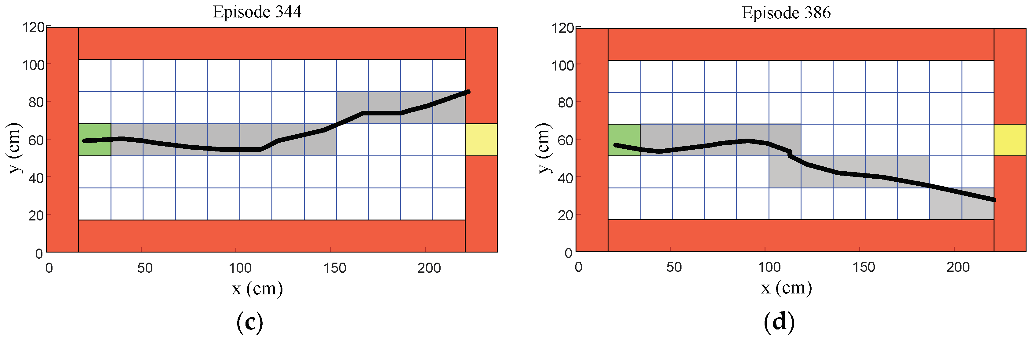
6.2. Middle Stage of the Learning Process

Episodes 201 to 400 represented the middle stage of the learning process, as shown in Figure 22. Episode 247 shows that the humanoid robot could gradually reach over half of the target distance, as shown in Figure 22a. After a few learning processes, episode 290 shows that the humanoid robot could reach the target region, as shown in Figure 22b. However, most episodes in the middle stage, such as episodes 344 and 386, show that the humanoid robot still could not reach the target region, as shown in Figure 22c,d.

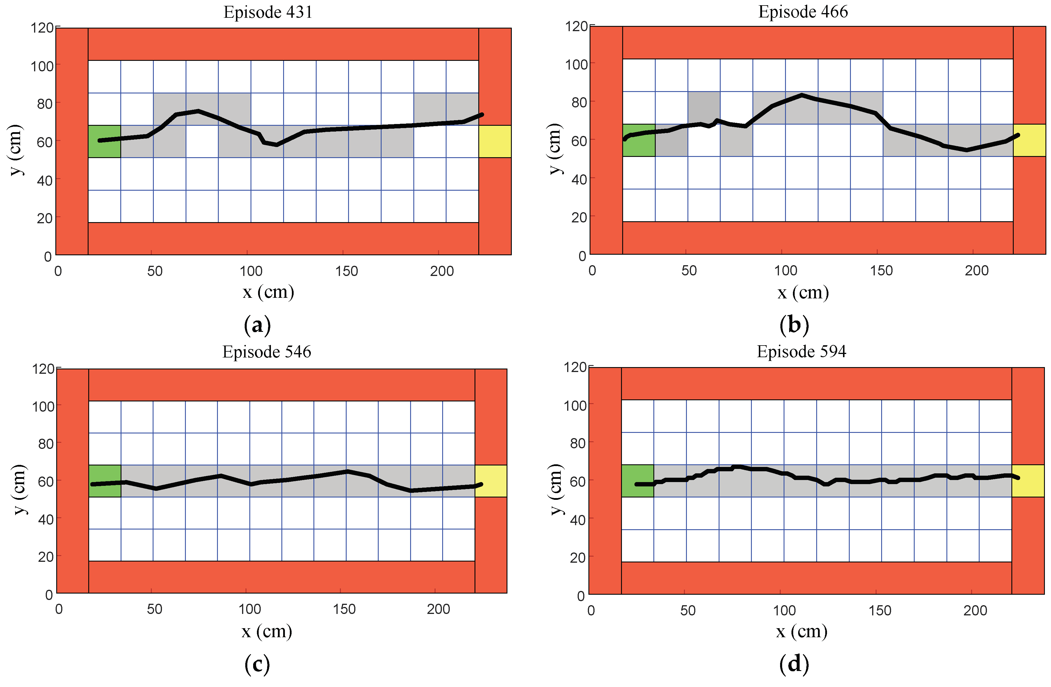
6.3. Final Stage of the Learning Process

Episodes 401 to 594 represented the final stage of the learning process, as shown in Figure 23. Episode 431 shows that the humanoid robot could gradually approach the target region, as shown in Figure 23a. After a few learning processes, episode 466 shows that the humanoid robot could reach the target region, as shown in Figure 23b. Moreover, most episodes in the final stage, such as episodes 546 and 594, show that the humanoid robot could not only reach the target region, but also walk approximately in a straight line, as shown in Figure 23c,d. Hence, the straightforward gait pattern was learned in this stage.

The recorded walking path could be analyzed based on the walking distance and the lateral offset. The walking distance was denoted by the horizontal length along the x-coordinate from the initial position to the end position. The lateral offset distance was the offset length compared with the straightforward line representing the walking distance. In the initial stage, the average walking distance was 95.4204 cm, which was far from the target region, and the average lateral offset distance was 22.8071 cm, which was also far from a straight line during this walking distance. In the middle stage, the average walking distance was 100.0183 cm, which approached the target region, and the lateral offset distance was 21.0969 cm, which also approached a straight line during this walking distance. In the final stage, the average walking distance was 148.7788 cm, which was closer to the target region, and the lateral offset distance was 14.8387 cm, which was closer to a straightforward line during this walking distance, within a unit coordinate of the training field. The detailed average experimental results are shown at each stage in

Table 6. Average experimental results at each stage (unit: cm).

Type	Initial stage	Middle stage	Final stage
Walking distance	95.4204	100.0183	148.7788
Lateral offset distance	22.8071	21.0969	14.8387

. The final Q-table of the straightforward gait pattern is shown in

Table 7. Final Q-table of the straightforward gait pattern.

$\begin{array}{cc}& \mathit{a}\\ \mathit{s}& \end{array}$		−7	−4	−2	−1	0	+1	+2	+4	+7
1	(0,0)	0.0000	−0.0036	−0.1000	0.0000	−0.0100	−0.0100	0.0000	−0.0100	0.0000
2	(1,0)	−0.2163	−0.2943	−0.1179	−0.1179	−0.2943	−0.2159	−0.2214	−0.1259	−0.2159
3	(2,0)	−0.2238	−0.2238	−0.3705	−0.2416	−0.2537	−0.2946	−0.3410	−0.2455	−0.2026
4	(3,0)	−0.2061	−0.3014	−0.3648	−0.2059	−0.2323	−0.2934	−0.2922	−0.2148	−0.1293
5	(4,0)	−0.2114	−0.2447	−0.3619	−0.3430	−0.3063	−0.4362	−0.3648	−0.3627	−0.2053
6	(5,0)	−0.2943	−0.2943	−0.2027	−0.4102	−0.3646	−0.3573	−0.2943	−0.2789	−0.1967
7	(6,0)	−0.1161	−0.2872	−0.2156	−0.2140	−0.2228	−0.2872	−0.2175	−0.1076	−0.2051
8	(7,0)	−0.0997	−0.2253	−0.2232	−0.2159	−0.2416	−0.1361	−0.1107	−0.1090	−0.1090
9	(8,0)	−0.1178	−0.2943	−0.3159	−0.2328	−0.3475	−0.4236	−0.2872	−0.2657	−0.1130
10	(9,0)	−0.2871	−0.3506	−0.4298	−0.3579	−0.2632	−0.3454	−0.2652	−0.4384	−0.1090
11	(10,0)	−0.1981	−0.2872	−0.2872	−0.2800	−0.2863	−0.2010	−0.2943	−0.4675	−0.1090
12	(11,0)	−0.1090	−0.4238	−0.4352	−0.2080	−0.1981	−0.2872	−0.2800	−0.1277	−0.1089
13	(0,1)	−0.0004	−0.0005	−0.0017	−0.0012	−0.0010	−0.0005	−0.0009	−0.0012	−0.0010
14	(1,1)	−0.0052	−0.0215	−0.0251	−0.0249	−0.0222	−0.0070	−0.0055	−0.0074	−0.0216
15	(2,1)	−0.0119	−0.0150	−0.0092	−0.1018	−0.0112	−0.0337	−0.0430	−0.0057	−0.0103
16	(3,1)	−0.0326	−0.0175	−0.0197	−0.0323	−0.0133	−0.0409	−0.0467	−0.0901	−0.0250
17	(4,1)	−0.0230	−0.0184	−0.0237	−0.0232	−0.0442	−0.0548	−0.0243	−0.0331	−0.0130
18	(5,1)	−0.0016	−0.0098	−0.0028	−0.0019	−0.0197	−0.0204	−0.0355	−0.0417	−0.0004
19	(6,1)	−0.0018	−0.0231	−0.0036	−0.0010	−0.0036	−0.0010	−0.0012	−0.0017	−0.0024
20	(7,1)	−0.0016	−0.0023	−0.0022	−0.0076	−0.0104	−0.0029	−0.0157	−0.0040	0.0002
21	(8,1)	−0.0047	−0.0200	−0.0639	−0.0172	−0.0229	−0.0507	−0.0405	−0.0312	0.0008
22	(9,1)	−0.0002	−0.0370	−0.0339	−0.0793	−0.0331	−0.0406	−0.0236	−0.0804	0.0000
23	(10,1)	0.0000	−0.0023	−0.0100	−0.0017	−0.0370	−0.0362	0.0000	0.0007	0.0000
24	(11,1)	−0.1981	−0.0100	−0.0100	−0.0500	−0.0099	−0.1323	−0.2080	−0.1000	0.0000
25	(0,2)	−0.0721	−0.2001	−0.0729	−0.0009	−0.0003	−0.0005	−0.0002	0.0005	−0.0010
26	(1,2)	−0.0002	−0.0007	−0.0009	−0.1601	−0.0003	−0.0006	0.0011	−0.1999	−0.0002
27	(2,2)	−0.0009	−0.0021	−0.0006	−0.0016	−0.0026	−0.0009	0.0019	−0.0003	−0.0006
28	(3,2)	0.0000	−0.0011	0.0026	−0.0010	−0.0012	−0.0011	−0.0018	−0.0010	−0.0012
29	(4,2)	0.0000	0.0001	−0.0001	0.0000	−0.0001	0.0000	−0.0020	−0.0021	0.0000
30	(5,2)	0.0000	−0.0008	−0.0002	0.0011	0.0000	0.0012	0.0000	0.0028	0.0000
31	(6,2)	0.0000	0.0011	0.0009	0.0000	0.0011	0.0031	0.0000	0.0000	0.0000
32	(7,2)	0.0000	0.0018	−0.0014	0.0008	0.0036	0.0000	0.0009	0.0000	0.0000
33	(8,2)	0.0005	0.0002	0.0007	0.0000	0.0000	0.0003	0.0003	0.0028	0.0000
34	(9,2)	0.0000	0.0002	0.0016	0.0043	0.0059	0.0130	0.0000	0.0000	0.0000
35	(10,2)	0.0090	0.0000	0.0000	0.0000	0.0000	0.0000	0.1908	0.0000	0.0774
36	(11,2)	0.0000	0.0910	−0.0001	0.0000	−0.0361	−0.0003	0.0000	0.6387	0.0628
37	(0,3)	0.0000	0.0000	0.0000	−0.0001	0.0000	0.0000	0.0000	0.0000	0.0000
38	(1,3)	−0.0017	−0.0001	−0.0025	0.0000	0.0000	−0.0016	−0.0001	−0.0001	−0.0001
39	(2,3)	−0.0008	−0.0008	−0.0014	−0.0022	0.0002	−0.0017	−0.0007	−0.0016	−0.0007
40	(3,3)	−0.0001	0.0011	−0.0008	−0.0005	−0.0009	−0.0007	−0.0008	−0.0046	−0.1000
41	(4,3)	−0.0006	−0.0034	−0.0008	0.0003	0.0018	−0.0036	−0.0002	−0.0014	−0.0006
42	(5,3)	0.0000	0.0008	0.0000	0.0000	0.0021	0.0000	0.0000	0.0000	0.0000
43	(6,3)	0.0000	0.0000	0.0026	0.0000	0.0000	0.0000	0.0000	0.0000	0.0000
44	(7,3)	0.0000	0.0000	0.0026	0.0000	0.0000	0.0000	0.0000	0.0000	−0.0100
45	(8,3)	0.0000	0.0001	0.0000	0.0000	0.0037	0.0001	0.0000	0.0000	0.0000
46	(9,3)	0.0000	0.0000	0.0000	0.0000	−0.0075	0.0000	0.0000	0.0087	0.0000
47	(10,3)	0.0000	0.0015	0.0000	0.0324	0.0000	0.0000	−0.0090	−0.0009	0.0000
48	(11,3)	−0.0100	−0.0100	−0.1981	−0.0100	−0.0100	−0.1090	0.0819	−0.1000	−0.1090
49	(0,4)	0.0000	0.0000	0.0000	0.0000	0.0000	0.0000	0.0000	0.0000	0.0000
50	(1,4)	−0.0100	−0.0100	−0.1089	−0.1008	−0.0197	−0.0199	−0.1022	−0.0100	−0.0100
51	(2,4)	−0.0173	−0.0199	−0.1156	−0.0989	−0.0284	−0.1090	−0.1179	−0.0986	−0.0199
52	(3,4)	−0.0093	−0.0100	−0.1066	−0.0181	−0.0485	−0.2078	−0.2061	−0.0100	−0.1089
53	(4,4)	−0.2158	−0.1138	−0.2159	−0.1056	−0.2154	−0.1154	−0.1081	−0.1146	−0.1090
54	(5,4)	−0.0100	−0.0907	−0.1088	−0.1000	−0.1014	−0.1000	−0.0100	−0.1000	−0.0100
55	(6,4)	−0.0100	−0.1000	−0.0100	−0.0179	−0.1511	−0.0090	−0.0100	−0.0073	−0.0100
56	(7,4)	0.0000	0.0000	0.0000	0.0000	−0.0100	−0.0100	0.0000	−0.1000	−0.0081
57	(8,4)	−0.0100	0.0002	0.0000	−0.0100	−0.0100	−0.1900	−0.0100	−0.0100	0.0000
58	(9,4)	0.0000	0.0000	0.0000	0.0000	−0.0100	−0.0001	−0.1000	−0.0006	0.0000
59	(10,4)	−0.1000	−0.1008	−0.0100	−0.1000	−0.1089	−0.0100	−0.0100	−0.0100	−0.1000
60	(11,4)	−0.0100	−0.1000	−0.1000	−0.1000	−0.0199	−0.0100	0.0000	−0.1000	−0.0100

.

7. Conclusions

In this paper, the Q-Learning algorithm was applied to learn a straightforward gait pattern for a humanoid robot based on an automatic training platform. There were four main contributions of this research. Firstly, an automatic training platform, which was an original idea, was proposed and implemented so that the humanoid robot could learn the straightforward walking gait in a real situation. Moreover, it could be used to reduce human resources and protect the humanoid robot in the training process. Secondly, a learning framework was proposed for the humanoid robot based on the proposed automatic training platform. Thirdly, an oscillator-based gait pattern was designed and combined with the proposed learning framework to reduce the number of learning parameters and speed up the learning process. Lastly, the Q-learning algorithm was applied in the proposed learning framework to allow the humanoid robot to learn the straightforward walking gait in a real situation. The proposed learning framework and automatic training platform were completely tested on a real small-sized humanoid robot, and an experiment was set up to verify its performance. In the learning process, the walking distance kept increasing, which shows that the humanoid robot could learn to walk toward the target region. Similarly, the lateral offset distance kept decreasing, which represents that the humanoid robot could walk in a straightforward pattern. From the experimental results of successful bipedal locomotion with a straightforward gait pattern, the feasibility of the proposed learning framework and automatic training platform could be validated. Hence, the desired behavior could be learned for the intrinsically unstable humanoid robot using the proposed learning framework, which could reduce human resources by using the automated learning process based on the proposed automatic training platform. The main purpose of this paper was to enable the robot to learn the straightforward gait pattern. When the robot is able to walk straight, it can then be combined with localization algorithms, such as Simultaneous Localization And Mapping (SLAM) and particle filter, in the future. The successfully learned straightforward gait pattern can be used in the localization algorithm to enable the robot to actually reach a specified position. Moreover, deep reinforcement learning can be designed and deployed in the proposed learning framework via the FPGA chip.