Abstract
Power-inversion (PI) adaptive arrays are widely used in Global Navigation Satellite System (GNSS) receivers for interference mitigation. The effects of element patterns on the performance of PI adaptive arrays are investigated in this paper. To this end, the performance of adaptive arrays is investigated by Monte Carlo simulations, using CST Microwave Studio (Dassault Systems, Vélizy-Villacoublay, France) to calculate the radiation patterns of circular microstrip elements which are used to compute the adaptive weight and the adaptive array gain. It is shown that the performance of PI adaptive arrays is mainly dependent on the gain pattern of the reference antenna element rather than the non-reference elements because the algorithm essentially pushes the elements into an unequal position. Furthermore, the results show that the impact of mutual coupling on the performance of the antenna array can be associated with the radiation patterns of the reference element, which is helpful in selecting the optimum reference element without increasing computational complexity, especially for small GNSS arrays.
1. Introduction
Global Navigation Satellite System (GNSS) adaptive antenna arrays have been acknowledged to be one of the most effective anti-interference options [1]. In an adaptive array, multiple antenna elements are employed to mitigate interfering signals spatially by steering nulls along the directions of interfering signals [2]. The total received signal of each antenna element is multiplied by the complex weight from the corresponding adaptive algorithms after being sampled and quantized by the radio frequency (RF) front-end of GNSS receivers.
Several effective adaptive algorithms for GNSS arrays have been proposed in many studies [3,4,5,6]. Among them, the power-inversion (or power minimization) (PI) algorithm [7,8,9] is very popular since it is relatively simple to implement and can effectively suppress interference without any prior information [10]. It should be pointed out that most analyses of the PI algorithm focus on the calculation scheme to find the optimal weight vector, and the elements of the array are assumed to be ideally isotropic.
However, it is recognized that the performance of adaptive antenna arrays is affected by the radiation patterns of antenna elements and the array geometry [11]. The radiation characteristics of element patterns should not be ignored. The accurate understanding of the in-situ response of individual antenna elements is complex and important, including mutual coupling between antenna elements and the scattering from the platform on which the antenna array is installed [12].
Furthermore, a comprehensive understanding of the impact of antenna element patterns on adaptive array performance is helpful in designing more effective antenna arrays. Firstly, it is helpful to select an optimum reference element for the PI algorithm. The results in [13] show that the effects of selecting a reference element on interference mitigation can be ignored, while the effects on the adaptive array gain cannot be neglected. The available angular region [14] of the adaptive array will be improved by selecting an optimum element. Youda Wan et al. proposed an improved PI algorithm based on optimum reference element selection [15]; however, this makes the adaptation process much more sophisticated. Secondly, it is helpful to determine whether mutual coupling would affect the array performance. Many designers have endeavored to minimize the mutual coupling between elements as a guideline [16,17], while others have started to treat the array as a whole aperture [18,19]. There is still a lack of a criteria for judging the impact of mutual coupling on the capability of antenna arrays.
In this paper, we specifically investigate the effects of the element radiation patterns on the performance of the adaptive array; in particular, we focus on the adaptive array gain. We illustrate that the output adaptive array gain is mainly dependent on the pattern of the reference antenna element rather than non-reference elements. We show that if mutual coupling deteriorates the reference element radiation pattern of a PI adaptive antenna array, the adaptive array performance will be considerably degraded. This finding not only provides inspirations to design better geometries, especially for small GNSS adaptive arrays, but also helps in choosing an optimum reference element to improve the performance of the array.
The remainder of this paper is organized as follows. The theoretical models for the PI adaptive arrays are given in Section 2. In Section 3, the performance evaluation of the arrays with different radiation patterns of elements is carried out. Section 4 is dedicated to explaining how the mutual coupling deteriorates PI adaptive arrays. The use of the findings in Section 4 to improve the adaptive array performance is discussed in Section 5. Finally, some useful conclusions are presented in Section 6.
2. PI Adaptive Array Model
In PI, a reference element is usually selected to avoid the all-zero solution of the weight vector, and its corresponding weight is fixed as 1. To find the optimum weight vector, the linear constraint minimum variance approach [1] is utilized. When the n-th element is chosen as the reference element, the weight vector can be expressed as [10]
where is the covariance matrix of the received signal , and is an inconsequential scalar, which will be ignored later in this paper. is a constraint vector with zeros except for the n-th element, with the value of 1 corresponding to the reference antenna.
It is assumed that and are the gain pattern and the phase pattern of the n-th element to a signal incident from direction , respectively. The pattern response of n-th element is denoted as follows:
Since there are J interfering plane waves, the total array response to the interference is defined as a matrix:
in which the j-th column is the array response vector to the j-th interference for , given by
where defines the incident angle of the j-th interference, is the position of the n-th element’s phase center for , and is the wavevector of the j-th interferer incident from direction , given in Cartesian coordinates by
Similarly, the array response vector to the desired signal is defined by
where the desired GNSS satellite signal incident along the direction and is the wavevector of the desired signal analogous to that for the interferer.
Therefore, the total received signal vector can be decomposed as
where represents the desired satellite signal, represents the j-th interference plane waves, and denotes the noise, which is modeled to be a Gaussian random variable with a zero mean and variance. It is assumed that the desired signal, interferences and noise are uncorrelated.
The desired satellite signal is so weak that its power is at least 20 dB less than the noise. Therefore, the covariance matrix can be simplified by neglecting the signal component as follows:
where reflects the power values of the interference signals. We assume that the powers of interferences are much stronger than the noise. Using the matrix inversion lemma in [20] to invert Equation (8), we obtain
where represents an orthonormal basis for the J-dimensional complex space scanned from . Note that
The situation in the presence of one single interferer is now considered to show the specific relationship between the adaptive array response and element patterns. We take the first element as the reference element; for example, in Equation (1) is equal to here. The weight vector may be calculated by substituting Equations (3) and (9) into Equation (1) as follows:
Therefore, the adaptive array pattern can be given as follows:
Combining Equations (6) and (11) gives
in which and .
Ideally, it is usually considered that the patterns of different elements are perfectly equal; i.e., . For this extreme case, Equation (13) will be simplified as
where the adaptive array pattern can be expressed as the product of the element pattern and the array factor, which is related to the location of the element and the relative position between the elements and the incident signal.
In reality, the mutual coupling between the antenna elements and other non-ideal factors make the elements dissimilar. As shown in Equation (13), besides the array factor, the adaptive array gain is mainly dependent on the radiation pattern characteristics of the reference element and may be influenced by the extent to which element patterns change compared to the reference pattern.
3. The Impact of Element Patterns on Array Performance
To find the relationship between the radiation patterns of elements and the adaptive array performance, the output adaptive array gain in the presence of a desired signal and J interfering signals is studied. It should be pointed out that the impacts of the RF front-end are neglected, and we assume that all the signals are continuous waves.
In order to characterize the adaptation performance, the angular availability is employed as the performance metric in this paper, which is commonly adopted in the research into GNSS adaptive arrays. It is defined as the percentage of the angular region over the entire upper hemisphere, where the output adaptive array gain is equal to or exceeds a selected threshold [19].
Two different distributions of antenna elements, as shown in Figure 1, are considered in this paper, which are commonly used as the array geometry for GNSS antenna arrays. Note that the element distribution G1 consisted of elements that are equally spaced on a circle with a half-wavelength radius (i.e., d = 0.5 as shown in Figure 1) and an element at the circle’s center. In element distribution G2, the antenna elements are uniformly spread on the perimeter of a circle with a radius of half a wavelength.
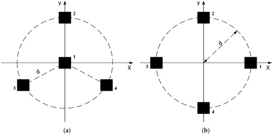
Figure 1.
Two array geometries: (a) G1; (b) G2.
The square patch element is located on a substrate with a height of 5 mm and a relative dielectric constant of 30. The patch element performs right-hand circular polarization (RHCP) by a dual-feed configuration providing two ports with a 90-degree phase difference. All the patch elements work at 1268.52 MHz, which is the central frequency of the B3 signal of the BeiDou Satellite Navigation System [21], and their S11 < −15 dB. We used CST Microwave Studio (Dassault Systems, Vélizy-Villacoublay, France) to simulate the in-situ response of elements in arrays, which is used to investigate the performance of the adaptive arrays through 100 Monte Carlo simulations in MATLAB (Mathworks, Natick, MA, USA). As shown in Figure 2, the incident angles of the interfering signals in each simulation are randomized uniformly from the region below 30° elevation, which is the common scenario in practice, while the incident angles of the GNSS signal vary in one-degree steps throughout the entire upper hemisphere. The average availabilities are finally calculated over 100 independent trials. For all simulations, it is assumed that the GNSS signal is 20 dB below the noise floor, and the interference signals are 40 dB above the noise.
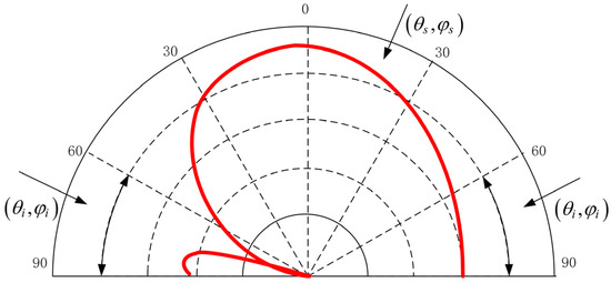
Figure 2.
Diagram of the incident directions of signals.
3.1. Gain Patterns
Firstly, the performance of the arrays with different gain patterns of elements is studied, and the effects of phase patterns are neglected here. By changing the size of the antenna aperture, we designed four different antenna elements, named E1, E2, E3 and E4, in CST Microwave Studio (Dassault Systems, Vélizy-Villacoublay, France) (see Figure 3), and the radiation patterns of these are shown in Figure 4. These four elements are selected as the reference elements of G1 and G2, respectively. Note that the reference elements are both located at element 1 as shown in Figure 1 and the other elements are equal.
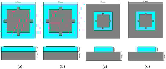
Figure 3.
Diagram of four differently sized antenna elements: (a) E1; (b) E2; (c) E3; (d) E4.
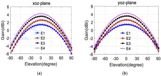
Figure 4.
Gain patterns of the four different antenna elements in Figure 3: (a) xoz-plane; (b) yoz-plane.
In Figure 5, the average angular availabilities of arrays with different gain patterns of reference elements are shown as a function of the values of the selected threshold Gth, for the case of G1 and G2, respectively. The results are shown for different numbers of RFIs (radio frequency interferences) in each case. It can be seen from Figure 5 that the availability improves with the increase of the gain of reference elements under the selected array geometries.
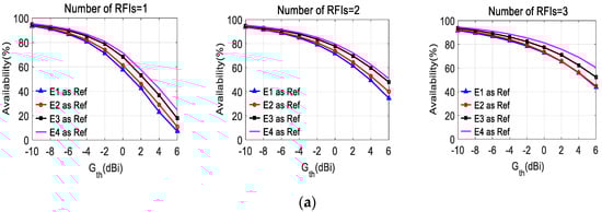
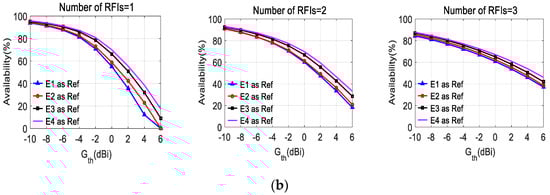
Figure 5.
Angular availabilities of arrays with different gain patterns of reference elements, as a function of Gth, for different numbers of radio frequency interferences (RFIs): (a) G1; (b) G2.
Next, we consider the impact of the extent of the change of non-reference element patterns as compared with the reference pattern on the array performance.
We selected the four elements in Figure 3 as non-reference elements of G1 and G2, respectively. Note that, in each case, the non-reference elements are identical (E1 or E2 or E3 or E4), and the gain patterns of these are shown in Figure 4. All reference elements are selected as E1 in different cases and are still located at element 1 as shown in Figure 1.
Figure 6 plots the performance of the antenna arrays with different gain patterns of non-reference elements. With the non-reference elements selected from E1 to E4, the gain patterns of the non-reference elements vary increasingly compared with those of the reference element, but the availabilities of the array remain nearly the same. It can be concluded that the extent of non-reference element gain pattern changes as compared with the reference pattern has little effect on the availability performance of the array.
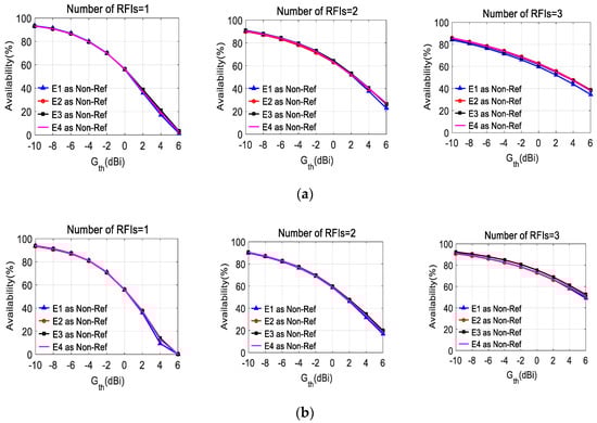
Figure 6.
Angular availabilities of arrays with different gain patterns of non-reference elements, as a function of Gth, for different numbers of RFIs: (a) G1; (b) G2.
Furthermore, it can be seen clearly from the comparison of Figure 5 and Figure 6 that the adaptive array gain of the PI array is mainly determined by the radiation pattern of the reference element, while the gain patterns of non-reference elements have little effect on the availability performance of the adaptive array. The good agreement between the results and the theoretical derivation in Section 2 evidently illustrates that the PI algorithm essentially forces the elements to be in an unequal position This leads to the domination of the radiation characteristics of the reference element on the adaptive array gain.
It should be pointed out that the larger the number of RFIs is, the smaller the effect of the gain of the reference element on the adaptive array gain. As depicted in Figure 5, the availability performance of the array is mainly dependent on the array factor when the number of interferences is equal to three. Overall, the adaptive array gain of G1 is slightly better than that of G2, as plotted in Figure 5 and Figure 6.
3.2. Phase Patterns
Secondly, the performance of arrays with different phase patterns of antenna elements is investigated. The effect of gain patterns is neglected here. Since the phase is a relative concept, we usually take the zenith direction as the zero-phase reference point. Additionally, the phase pattern of the patch antenna in this paper has some characteristics that are nearly unchanged with the increase of elevation angle; however, the phase will fluctuate with the increase of elevation angle as the patch antenna is located in the array. The phase pattern comparison between the ideal patch antenna and the real element in array is depicted in Figure 7. Note that the phase fluctuation of the real antenna in the array with the increase of elevation angle is generally from 0 to 30 degrees compared to the zero-phase reference point. According to this characteristic, we artificially designed four different antennas, named E5, E6, E7 and E8, the phase patterns of which are shown in Figure 8.
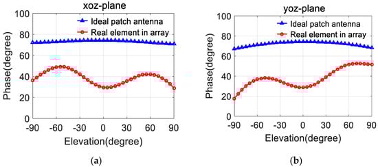
Figure 7.
Phase pattern comparison of the ideal patch antenna and the real element in the array: (a) xoz-plane; (b) yoz-plane.
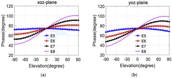
Figure 8.
Phase patterns of four different antenna elements: (a) xoz-plane; (b) yoz-plane.
We selected these four elements as the reference elements of G1 and G2, respectively. Note that the reference elements are both located at element 1, as shown in Figure 1, and the other elements are equal. In Figure 9, the average angular availabilities of arrays with different phase patterns of reference elements are presented for the case of G1 and G2, respectively. The results are shown for different numbers of RFIs in each case.
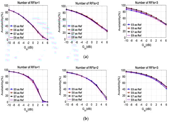
Figure 9.
Angular availabilities of arrays with different phase patterns of reference elements, as a function of Gth, for different numbers of RFIs: (a) G1; (b) G2.
Similarly, these four elements are selected as the non-reference elements of G1 and G2, respectively. Figure 10 plots the performance of the antenna arrays with different phase patterns of non-reference elements, which are selected from Figure 8. Note that in different cases, the non-reference elements are identical (E5 or E6 or E7 or E8); the phase patterns are shown in Figure 8. Furthermore, all reference elements are selected as E5 and are still located at element 1, as shown in Figure 1.
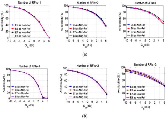
Figure 10.
Angular availabilities of arrays with different phase patterns of non-reference elements, as a function of Gth, for different numbers of RFIs: (a) G1; (b) G2.
Obviously, both the phase pattern of the reference element and the non-reference elements have little effect on the availability performance of the PI adaptive array. The results in Figure 9 and Figure 10 illustrate that the PI algorithm has a certain adaptability to the phase perturbation of the elements.
Conventionally, as the number of RFIs increases, the availability will degrade since more nulls should be steered towards interferer sources. However, the availabilities in Figure 5, Figure 6, Figure 9 and Figure 10 increase as the number of RFIs increases. To explain this phenomenon, we choose three specific scenarios in which the numbers of RFIs are one, two, and three, respectively: (a) ; (b) and ; (c) , and .
Figure 11 plots the adaptive gain of the four-element array (G1) towards the direction of the interferences in the specific scenes. Furthermore, the elements in the array are all selected as E1. As shown in Figure 10, the nulling (about −90 dB) in the presence of one interference is much deeper than that (about −50 dB) when there are two or three interferences. This deeper nulling will cause the region where the adaptive array gain is less than the threshold to become much larger, as depicted in Figure 12. On the other hand, the maximum array gains in Figure 12a–c are 7.24 dB, 8.03 dB and 15.35 dB, respectively; that is, the array gain will be larger in a region far from the nulling as the number of RFIs increases. In summary, the availability will increase and the nulling capability will decrease as the number of RFIs increases.
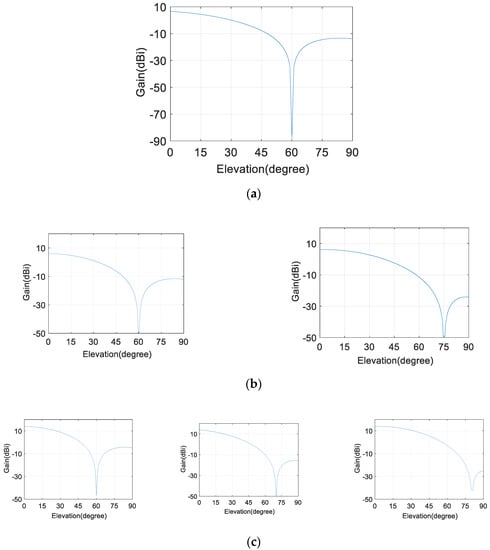
Figure 11.
The nulling capability of the four-element array: (a) number of RFIs = 1; (b) number of RFIs = 2; (c) number of RFIs = 3.
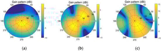
Figure 12.
The adaptive array gain patterns of the four-element array: (a) number of RFIs = 1; (b) number of RFIs = 2; (c) number of RFIs = 3.
Figure 11 plots the adaptive gain of the four-element array (G1) towards the direction of the interferences in the specific scenes. Furthermore, the elements in the array are all selected as E1. As shown in Figure 10, the nulling (about −90 dB) in the presence of one interference is much deeper than that (about −50 dB) when there are two or three interferences. This deeper nulling will cause the region where the adaptive array gain is less than the threshold to become much larger, as depicted in Figure 12. On the other hand, the maximum array gains in Figure 12a–c are 7.24 dB, 8.03 dB and 15.35 dB, respectively; that is, the array gain will be larger in a region far from the nulling as the number of RFIs increases. In summary, the availability will increase and the nulling capability will decrease as the number of RFIs increases.
We suggest that the primary reason for this phenomenon may be the number of elements in the array being insufficient. We can improve the nulling capability by employing more elements in the array. As shown in Figure 13, two more elements are added to the four-element array in Figure 10 (other conditions are unchanged), and the nulling capability of the new six-element array did not decrease dramatically as the number of RFIs increased. In this case, the array gain and the availability obviously decreased, as depicted in Figure 14, because the deeper nullings are steered as expected.
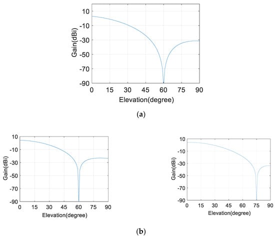
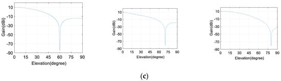
Figure 13.
The nulling capability of the six-element array: (a) number of RFIs = 1; (b) number of RFIs = 2; (c) number of RFIs = 3.
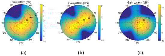
Figure 14.
The adaptive array gain pattern of the six-element array: (a) number of RFIs = 1; (b) number of RFIs = 2; (c) number of RFIs = 3.
According to the analysis mentioned earlier, the availability sometimes cannot characterize the array performance comprehensively. The nulling capability may decrease when the availability improves; therefore, it is more meaningful to investigate the availability of antenna arrays with the same number of interferences and elements. Moreover, we should combine the null deepness and the availability to judge the performance of PI adaptive arrays so that we can investigate the antenna array comprehensively and fairly.
4. The Impact of Mutual Coupling on Array Performance
The effect of mutual coupling between the elements is neglected in the above experiments to verify the theoretical derivation in Section 2 using a relatively ideal pattern of patch elements. The mutual coupling between small arrays often influences impedance matching, resonant frequency, and especially the element patterns, leading to the degradation of the adaptive array gain.
According to the results mentioned above, the PI adaptive array gain is mainly related to the radiation characteristics of reference elements rather than non-reference elements. Thus, we are interested in comparing the adaptive array performance related to different mutual couplings which results in different patterns of reference elements.
As depicted in Figure 15, five-element patch arrays were designed in CST Microwave Studio (Dassault Systems, Vélizy-Villacoublay, France) using the array geometries in Figure 1. One more element is added to G1 and G2 to increase the mutual coupling between elements. Note that the reference elements are both located at element 1, as shown in Figure 15, and the radii of the array are 0.5 , 0.3 and 0.25 , respectively. The other experimental conditions are the same as those in Section 3.
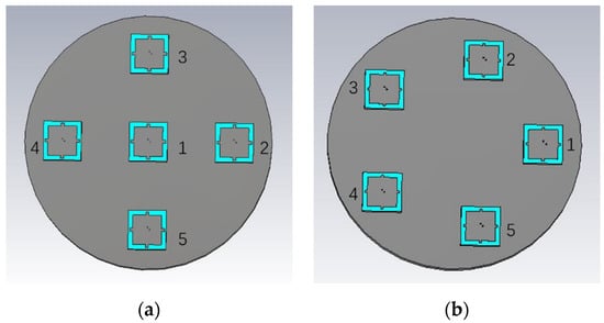
Figure 15.
Five-element patch array model using the array geometries in Figure 1: (a) A1; (b) A2.
It can be seen from Figure 16 that, as the interelement spacing decreases, the performances of the five-element patch arrays gradually deteriorate. Especially when the radius is 0.25 , the availability of G1 and G2 both decrease much more significantly than when the radius is 0.5 , since the strong mutual coupling between elements comes into play. Moreover, the comparison of Figure 16a,b illustrates that the performances of A1 and A2 nearly stay the same due to the small mutual coupling when the interelement spacing is of the order of half a wavelength. However, the availability of A1 obviously deteriorates compared with that of A2 when the elements become more closely packed.
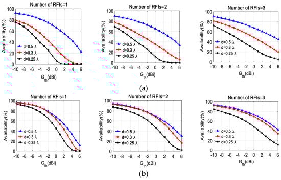
Figure 16.
Angular availability comparison of arrays with different array aperture sizes, as a function of Gth, for different numbers of RFIs. (a) A1; (b) A2.
Figure 17 shows the radiation characteristic comparison of reference elements in A1 and A2 when the radii are 0.3 and 0.25 , respectively. Given that the reference element located at the center will be more severely affected by mutual coupling than that spread on the perimeter of the circle, the gain of the reference element in A1 tends to degrade more seriously than that in A2 when the aperture size decreases.
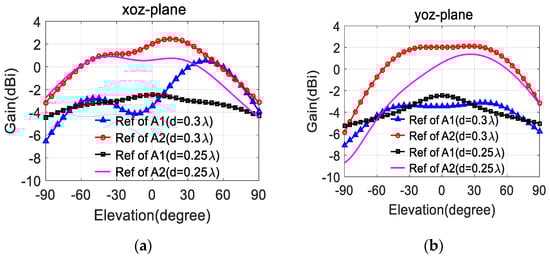
Figure 17.
Radiation patterns of reference elements of arrays A1 and A2 with different aperture sizes (d = 0.3 and d = 0.25 , respectively): (a) xoz-plane; (b) yoz-plane.
We can draw the following conclusion from the above results: if the mutual coupling deteriorates the radiation pattern of the reference element of the PI adaptive antenna array, the performance of the adaptive array gain and availability will considerably degrade. In practice, this finding is very important, in that the total effect of mutual coupling on the overall antenna array performance can be associated with the patterns of the reference element. According to this conclusion, it is possible to design a more reasonable small PI antenna array geometry which should avoid the potential degradation of the radiation pattern of the reference element by mutual coupling; for example, A2 is a better choice than A1, especially when reducing the size of the antenna array.
5. Discussion
For small antenna arrays, the selection of a reference element should consider the absolute in-situ response of individual antenna elements. In practice, the optimum reference elements could be selected according to the measured radiation patterns of different elements in the array, and it is not necessary to employ a sophisticated algorithm, such as the algorithm proposed in [15], which will be unsuitable for small antenna arrays due to the increased computational complexity. For example, we can improve the poor performance of array A1 when the radius is 0.25 by choosing an element with a better gain pattern. As shown in Figure 18, element 2 in Figure 15a is more suitable as a reference element than element 1 for array A1, which is verified by the results presented in Figure 19. The results are consistent with our previous analysis; i.e., the in-situ radiation pattern of an element will help us select the optimum reference element while avoiding exhaustive tests or sophisticated algorithms.
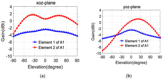
Figure 18.
Radiation patterns of element 1 and 2 of A1 (d = 0.25 ): (a) xoz-plane; (b) yoz-plane.
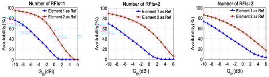
Figure 19.
Angular availability comparison of array A1 (d = 0.25 ) with different reference elements, as a function of Gth, for different numbers of RFIs.
6. Conclusions
This paper investigated the impact of element patterns on the performance of GNSS power-inversion adaptive arrays. It is shown that the availability of PI adaptive arrays is mainly dependent on the gain pattern of the reference antenna element rather than the non-reference elements. Additionally, the PI algorithm is not sensitive to the phase perturbation of the elements. Furthermore, the results presented in this paper verified that if the strong mutual coupling between the elements deteriorates the gain performance of the reference element, the availability of PI adaptive arrays will be degraded accordingly. This finding permits us to improve the performance of an adaptive array by observing the pattern characteristics of elements rather than by thoroughly testing a large number of required signals and jammer scenarios.
Author Contributions
Conceptualization, L.L. and S.N.; Data curation, J.L.; Formal analysis, J.L.; Funding acquisition, S.N.; Investigation, Z.L.; Methodology, J.L.; Project administration, S.N.; Resources, F.C.; Software, J.L.; Supervision, S.N.; Validation, Z.L. and F.C.; Visualization, L.L.; Writing—original draft, J.L. and L.L.; Writing—review and editing S.N. Z.L. and F.C.
Funding
This work was supported by the National Natural Science Foundation of China (no. 61601485).
Conflicts of Interest
The authors declare no conflict of interest. The funders had no role in the design of the study; in the collection, analyses, or interpretation of data; in the writing of the manuscript, or in the decision to publish the results.
References
- Navid, R.; Lotfollah, S. Impact of element pattern symmetry on the effective degrees of freedom in dual-polarized gnss adaptive antenna arrays. IEEE Trans. Antennas Propag. 2018, 66, 4669–4677. [Google Scholar]
- Fernández-Prades, C.; Arribas, J.; Closas, P. Robust gnss receivers by array signal processing: Theory and implementation. Proc. IEEE 2016, 104, 1207–1220. [Google Scholar] [CrossRef]
- Zoltowski, M.D.; Gecan, A.S. Advanced adaptive null steering concepts for GPS. In Proceedings of the IEEE Military Communications Conference, San Diego, CA, USA, 5–8 November 1995; pp. 1214–1218. [Google Scholar]
- Fante, R.L.; Vaccaro, J.J. Wideband cancellation of interference in a gps receive array. IEEE Trans. Aerosp. Electron. Syst. 2000, 36, 549–564. [Google Scholar] [CrossRef]
- Amin, M.G.; Wei, S. A novel interference suppression scheme for global navigation satellite systems using antenna array. IEEE J. Sel. Areas Commun. 2005, 23, 999–1012. [Google Scholar] [CrossRef]
- O’Brien, A.J.; Gupta, I.J. An optimal adaptive filtering algorithm with zero antenna-induced bias for gnss antenna arrays. Navigation 2010, 57, 87–100. [Google Scholar] [CrossRef]
- Compton, R.T., Jr. The power-inversion adaptive array: Concept and performance. IEEE Trans. Aerosp. Electron. Syst. 1979, AES-15, 803–814. [Google Scholar] [CrossRef]
- Gecan, A.; Zoltowski, M. Power minimization techniques for GPS null steering antenna. In Proceedings of the 8th International Technical Meeting, ION GPS-95, Palm Springs, CA, USA, 12–15 September 1995; pp. 861–868. [Google Scholar]
- Carrie, G.; Vincent, F.; Deloues, T.; Pietin, D.; Renard, A. A new blind adaptive antenna array for GNSS interference cancellation. In Proceedings of the 39th Asilomar Conf. Signals, System, Computers, Pacific Grove, CA, USA, 28 October–1 November 2005; pp. 1326–1330. [Google Scholar]
- Xu, H.; Cui, X.; Lu, M. Effects of power inversion spatial only adaptive array on gnss receiver measurements. Tsinghua Sci. Technol. 2018, 23, 172–183. [Google Scholar] [CrossRef]
- Gupta, I.J.; Ulrey, J.A.; Newman, E.H. Effects of antenna element bandwidth on adaptive array performance. IEEE Trans. Antennas Propag. 2005, 53, 2332–2336. [Google Scholar] [CrossRef]
- Gupta, I.J.; Weiss, I.M.; Morrison, A.W. Desired features of adaptive antenna arrays for gnss receivers. Proc. IEEE 2016, 104, 1195–1206. [Google Scholar] [CrossRef]
- Feiqiang, C.; Junwei, N.; Xiangwei, Z. Impact of reference element selection on performance of power inversion adaptive arrays. In Proceedings of the 2016 IEEE/ION Position, Location and Navigation Symposium (PLANS), Savannah, GA, USA, 11–14 April 2016. [Google Scholar]
- Ulrey, J.A.; Gupta, I.J. Optimum Element Distribution for Circular Adaptive Antenna Systems. In Proceedings of the 2006 National Technical Meeting of The Institute of Navigation, Monterey, CA, USA, 18–20 January 2006. [Google Scholar]
- Wan, Y.; Chen, F.; Nie, J.; Sun, G. Optimum reference element selection for gnss power-inversion adaptive arrays. Electron. Lett. 2016, 52, 1723–1725. [Google Scholar] [CrossRef]
- Volakis, J.L.; O’Brien, A.J.; Chen, C.-C. Small and adaptive antennas and arrays for gnss applications. Proc. IEEE 2016, 104, 1221–1232. [Google Scholar] [CrossRef]
- Gheethan, A.A.; Herzig, P.A.; Mumcu, G. Compact 2 × 2 coupled double loop gps antenna array loaded with broadside coupled split ring resonators. IEEE Trans. Antennas Propag. 2013, 61, 3000–3008. [Google Scholar] [CrossRef]
- Griffith, K.A.; Gupta, I.J. Effect of mutual coupling on the performance of gps aj antennas. Navigation 2009, 56, 161–173. [Google Scholar] [CrossRef]
- Svendsen, A.S.; Gupta, I.J. The effect of mutual coupling on the nulling performance of adaptive antennas. IEEE Antennas Propag. Mag. 2012, 54, 17–38. [Google Scholar] [CrossRef]
- Gupta, I.J.; Ksienski, A. Dependence of adaptive array performance on conventional array design. IEEE Trans. Antennas Propag. 1982, 30, 549–553. [Google Scholar] [CrossRef]
- Xiao, W.; Liu, W.; Sun, G. Modernization milestone: Beidou m2-s initial signal analysis. Gps Solut. 2016, 20, 125–133. [Google Scholar] [CrossRef]
© 2019 by the authors. Licensee MDPI, Basel, Switzerland. This article is an open access article distributed under the terms and conditions of the Creative Commons Attribution (CC BY) license (http://creativecommons.org/licenses/by/4.0/).