GPU Acceleration and Game Engines for Wireless Channel Estimation in Millimeter Waves

Abstract

In this article, the intended purpose is to show an innovative technique for estimating the MIMO channel at millimeter wave bands, candidates for mobile 5G technology, by using hardware acceleration, game engines and heuristic algorithms applied to optical ray launching techniques. To verify the performance of the ray launching tool, the normalized Power Delay Profile (PDP) was simulated. The channel was analyzed using the mean square delay error (RMS), the average value of the delay (MD) and the basic propagation loss (PL). The results obtained in computational precision and time were compared with those of a traditional ray tracing tool simulation programmed in MATLAB and with the measurements made in the 57 to 66 GHz range in a specialized laboratory. The results show that the presented technique becomes efficiently profitable from a small number of simulated events (reflections, diffractions).

1. Introduction

Overcrowding in access to multimedia information such as online videogames and streaming services forces the next generation of communications to present technological advances quickly [1,2]. That is, increase the efficiency of the wireless channel through transmission in the shortest time and with an acceptable quality to the greatest number of possible users. Nowadays, rates between wireless LAN technologies and mobile networks are comparable, forcing a coexistence to avoid interference [3]. Therefore, they tend to integrate and become the same access technology.

5G mobile networks must face the challenges of energy consumption and high rates [4]. In compliance with the formulation in Shannon’s capacity, there are two ways to improve service quality: Increasing signal strength or increasing bandwidth.

The best way to improve energy consumption and, at the same time, increase the signal strength is through the implementation of femtocells [5]. Smaller coverage areas between the transmitter and the receiver improve signal strength and interference to provide better quality of service. In this paradigm, the difficulty of interference can be resolved with the use of a radio spectrum available at high frequencies and cognitive radio [6].

By the other way, spectral efficiency improves by increasing the bandwidth of the channel [7]. To solve the need bandwidth, mobile technologies have been increasing their operating frequencies as it evolves. The next mobile generation hopes to use millimeter waves or terahertz to improve the quality of service.

A relevant factor is the implementation of multiple antennas for the simultaneous transmission of information, using spatial multiplexing or diversity [8]. By means of a lower wavelength given by the millimeter or terahertz waves, it is possible to integrate a greater number of antennas and make them smaller. The MIMO and MIMO massive sets will support emerging technologies called next-generation mobile networks (NGMN).

To evaluate technological implementations, it is necessary to estimate the behavior of the radio channel through precise models such as deterministic models [9]. With the estimation of the radio channel at the physical layer level, support is provided for the choice of digital modulations, media access techniques and the encodings that will be used.

Radio channel estimation use stochastic or deterministic models. First models use a probabilistic distribution function and disregard some channel effects due to the antennas or the type and number of scatterers in the scenario to be evaluated. Deterministic models are adequate in different environments with scatterers of considerable size, given their exact and verifiable predictions [10]. Computational methods have had an enormous influence on the prediction of wireless channel parameters, with the optical beam technique being the most accurate [11]. Until now, the technique of ray tracing (RT) based on the image method [9,12,13] and the technique of ray launching (RL), which uses the brute force algorithm, have been implemented with greater efficiency and precision [14,15,16].

However, computationally, the first technique is limited to a simplified scenario due to the number of secondary sources (images) that are produced by the multiple reflection and diffraction phenomena. With respect to the second technique, its accuracy is based on the firing resolution angle. The rays produced initially and those generated as a secondary source, a product of the Huygens–Fresnel principle, exponentially increase the number of paths to analyze. For ray launching to be a practical, accurate and computationally efficient strategy, it is necessary to resort to the use of game engines and hardware acceleration, but such studies have been limited to the estimation of the wireless channels of a transmitter and a receiver (SISO, single input single output) in decimeter waves.

The above mentioned indicates that it is necessary to develop efficient and practical acceleration techniques that allow a reduction in the simulation time while maintaining accuracy. Each ray launched or traced is independent of the rest of the rays and, therefore, it is possible for a processor or processor unit to calculate the path and the interactions of one ray at the same time that another processor does the same with another ray. In this way, if several processors are available, the task of launching or tracing beams can be parallelized reaching a high efficiency without losing precision.

In Section 2 we present the materials and methods used to develop the software in the game engine using ray launching and the way in which the measurement campaign was carried out. In Section 3 the obtained results are described and compared with another optical ray strategy developed in MATLAB. In Section 4 we discuss some aspects of how this application would be in other environments. Finally, in Section 5 the conclusions are presented.

2. Materials and Methods

Next, we describe both the geometrical model of the stage and the physical model of wave propagation using game engines and hardware acceleration. The estimation of channel parameters depends, to a large extent, on these representations.

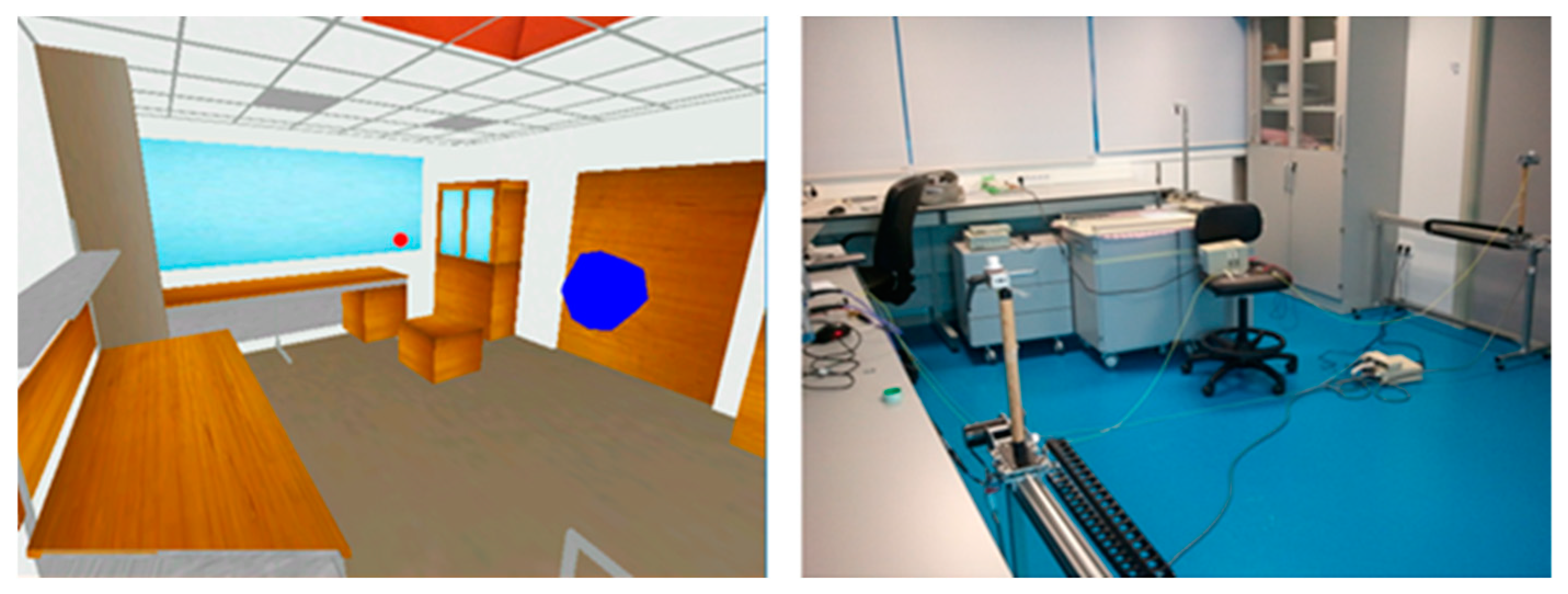
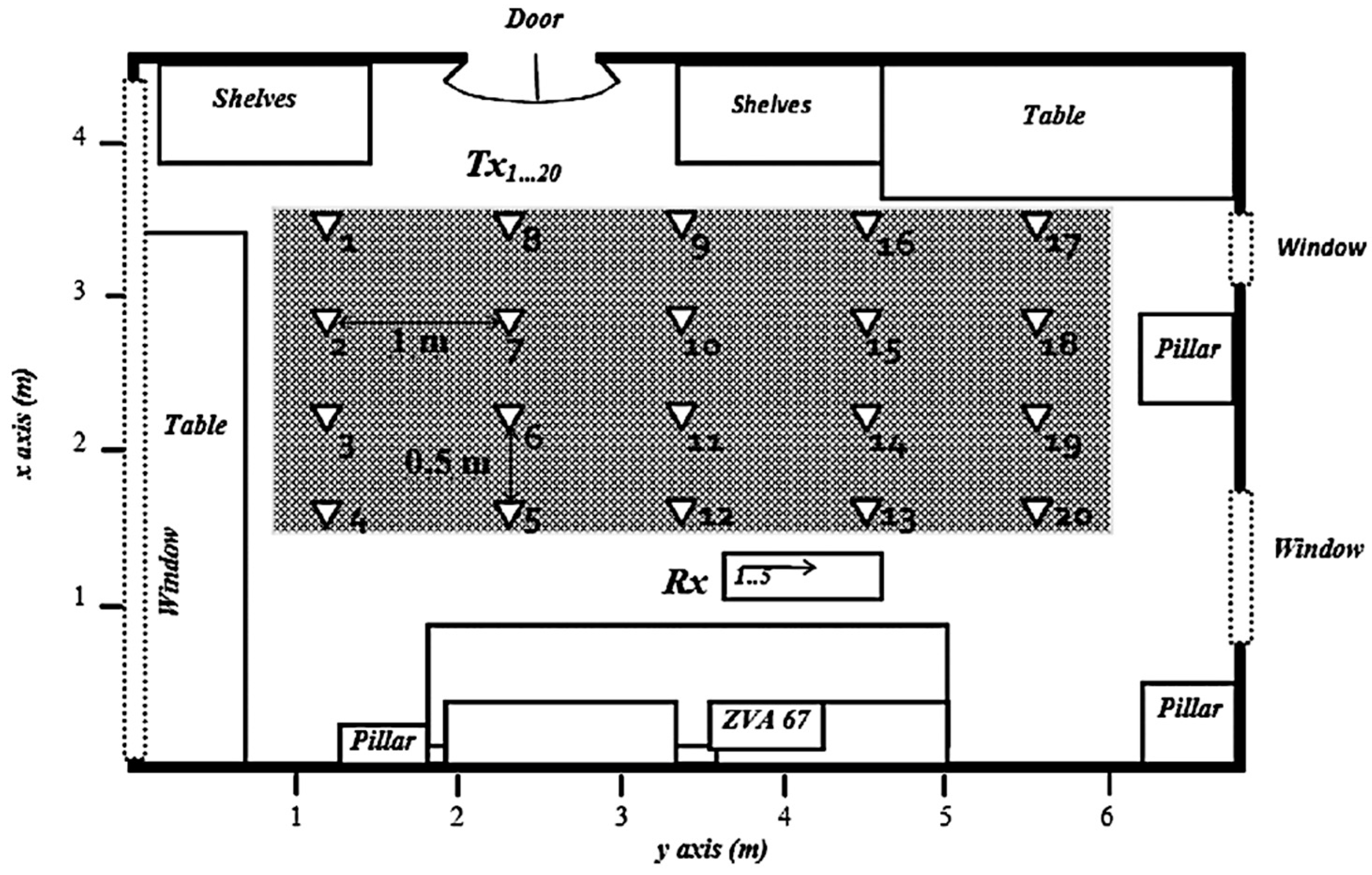
2.1. Description of the Test Scenario

The accuracy of the results of the ray launcher is intimately linked with the description of the environment or 3D scenario for both indoor and outdoor environments. The representation of the scatterers as well as their constitutive parameters must be included in a high-resolution model, and the representation must include both the electromagnetic characteristics of the materials and the dimensions of each one of the scenario elements.

Figure 1 shows a photograph (right) of the laboratory at the Polytechnic University of Cartagena (UPCT), Spain, used for measurements and its 3D computational model (left). The scenario has dimensions of 6.40 m x 4.44 m x 2.60 m. Five classes of materials present in the analysis scenario were identified. The floor and columns consist of concrete, glass windows, wooden furniture with metal frames and a plaster ceiling. On the left, the game engine representation is shown, where the red sphere represents the transmitter position and the blue sphere represents the receiver position (setup of 5 transmitting antennas) for a total of 180 MIMO channels.

The measurements were made at different locations inside the laboratory, as shown in Figure 2. Each one of the triangles (transmitters) represents a virtual uniform rectangular array (URA) composed of 6 x 6 positions, and the receiver is a virtual uniform linear array (ULA) composed of 1 x 5 positions. Thus, 180 MIMO channels were measured in each one of the locations. The separation distance between each location is 1 m in length and 0.5 m in width.

The initial values used for the relative permittivity and the conductivity of the scenario materials were provided by the UPCT advisors (mentioned in the Acknowledgments) and are shown in

Table 1. Values of relative permittivity and conductivity of materials.

Element	Relative Permittivity	Conductivity (S/m)
Floor and Columns	6.5–0.43i	1.43
Walls and Drop-Down Ceiling	2.81–0.046i	0.15
Furniture	1.54–0.095i	0.32
Metal	1	1
Glass	6.94–0.176i	0.59

.

In the literature, the nominal values of relative permittivity and conductivity for wood, concrete and glass can be found for specific materials and at low frequencies, far from the measurement frequencies. For this reason, measured values were taken in [12].

Figure 3 shows a scheme of the system used for the measurements. The frequency response is measured using a vector network analyzer. Then, the inverse Fourier transform is applied to obtain the complex impulse response (CIR) in the time domain. Once all CIRs are collected for one location the PDP is obtained as usual by averaging the CIRs. The range of measurements was between 57 GHz and 66 GHz with 4096 frequency points. The measurement system used consists of two groups of identical omnidirectional antennas in virtual arrays (Q-pair QOM55-65 VRA) with vertical polarization and gain ranging from 4 to 5.1 dBi along the bandwidth. In each array, the antenna elements, both in reception and transmission, are separated equidistantly 2 mm, which in terms of wavelengths gives a ratio of $\lambda /2$. In addition, the antennas have an omnidirectional radiation pattern in the H plane and a medium power beam centered at 40°, 28° and 21° for the frequencies of 55 GHz, 60 GHz and 65 GHz, respectively.

The antennas are supported on metal structures 1.44 m high for the transmitter and 1.54 m for the receiver. They are connected with a coaxial cable to the Rohde & Schwartz ZVA67 vector network analyzer whose transmission power was –10 dBm. To compensate for the attenuation effects of the coaxial cables, amplifiers (HXI HLNA-465) with maximum gains of 25 dB were used, whose effects were measured and adjusted. In order to obtain precision, a software was created for positioning with servomotors and operated from outside the environment to maintain the channel stationary. With an intermediate frequency of 10 Hz, a dynamic range of more than 100 dB was obtained.

The 3D model of the scenario was obtained using plane geometries to represent all the objects. Each of the physical geometries of the objects present in a laboratory can be modeled by combining some basic primitive geometries, which altogether achieve great geometric resolution. However, in the selected scenario, the environment and the present objects do not have great geometric complexity and are composed of flat surfaces with their respective properties of dimension, thickness, permittivity and conductivity. Likewise, to identify the impact of the propagation wave on the edges, a cylinder shape was used. Furthermore, to represent the measurement points and to identify the rays that impact on them, the geometry of the reception sphere was used.

The open source multiplatform tool Blender 2.74 was used to develop 3D modeling of the internal environment, which uses Python as an internal programming language. In a first phase, the data are selected to create the environment according to the measurements of the realistic UPCT scenario, obtaining the points of the XY coordinates with their respective height for each element that is included in the study environment.

In Blender each object is included by adding a cube-type mesh in the scene for the walls, floor, ceiling, windows and other elements of the environment. Additionally, each material is represented as textures that are incorporated in the model, by means of the texturing technique mapped in 2D coordinates (UV), which allows to establish a correspondence between the vertices of an object and the coordinates of a texture.

Assigning an image to each polygon according to the material in the model of the environment, to improve rendering, you get great 3D resolution providing realism to the scenario. Finally, before exporting the files, the transformations of scale, units, rotation and location of the scene applied in the 3D environment of Blender must be considered. This is important in order to apply the changes of the scene with the characteristics of the model as material, meshes and associated textures, to later import the model in the JME (Java Monkey Engine). Subsequently, the 3D scenario in Blender format is exported to a format compatible with the game engines.

2.2. Channel Modeling

The brute force method employed uses the theory of the optical beam that allows to separate each propagation mechanism (reflection, diffraction and dispersion) with the advantage of applying optical geometry. It is based on the SBR (Shooting and Bouncing Ray) algorithm. First, rays are launched from the transmitting antenna, and then the ray trajectories are traced, allowing us to see if it hits any object in the environment or if it reaches the receiving antenna. When the beam hits a flat surface, a reflected beam is generated and another transmitted by the interface, but if the beam hits an edge, a large amount of diffracted rays are generated and each of them is drawn until it hits another object and so on until it is discarded as having less power than the sensitivity of the receiver, or successfully impacting the receiver. Finally, the ray characteristics associated with the propagation are calculated.

The ray launching method applies the Fermat principle and the local field principle to model rays. Fermat’s principle states that a ray follows the shortest path from the source to the field point, while the principle of the local field states that when the rays strike a surface, they experience reflection, refraction and diffraction, and at high frequencies, it only depends on the electrical and geometric properties of the scatterers.

Each ray is associated with a complex and vectorial electric field of amplitude, which is computed taking into account the field emitted in the transmitter, the losses in the free space, the reflections, and the diffractions and diffusions experienced by the ray in which the appropriate models are used. The losses in the free space are represented by the Friss equation, and the reflections are represented by applying the Fresnel reflection coefficients, while for diffraction the vector field is multiplied by the relevant diffraction coefficients and obtained from the UTD theory, using a modification of Luebber’s coefficients.

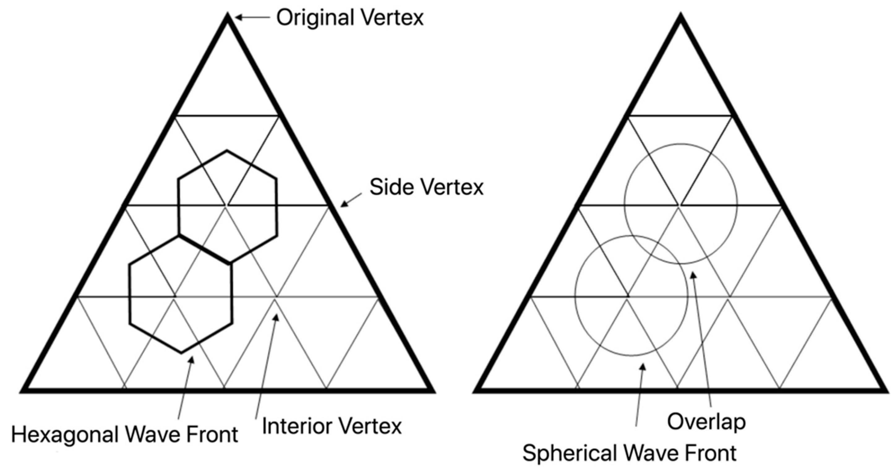
2.3. Ray Propagation

The transmitter is modeled as a source point. To determine all the possible rays that can be launched from the transmitter and reach the receiver it is necessary to consider all possible angles of the transmitter’s output and arrival at the receiver. The rays must be launched from the transmitter at an elevation angle and an azimuth angle relative to the fixed coordinate system and following a launch method.

The ray tracer calculates both the temporal dimension and the frequency. For purposes of the comparisons with the ray tracer of the UPCT and with the measurements, its operation is used in the frequency domain. Thus, the launcher calculates the gain in direct transmission of the electric field (parameter) under the following equation:

$$E_{rx}=S_{21}{E}_{tx}$$

(1)

where $E_{rx}$ is the electric field at the point of reception and $E_{tx}$ the electric field at the point of transmission. For this last situation the electric field is assumed as a phasor with a zero phase of reference. The power in the receiver is calculated by [17]:

$$P_{rx}=\frac{P_{tx}{G}_{tx}}{4\pi d^2}=\frac{{\left|E_{rx}\right|}^2}{120\pi }\raisebox{1ex}{$w$}\!\left/ \!\raisebox{-1ex}{$m^2$}\right.$$

(2)

but

$$\left|E_{rx}\right|=\frac{\sqrt{30P_{tx}{G}_{tx}}}{d}.$$

(3)

For all trajectories without line of sight (NLoS, Non-Line of Sight) you can write of (2) and (3):

$$\left|E_{rx}\right|=S_{21}\left|E_{tx}\right|$$

(4)

if the received power is considered at a specific distance

$$P_{rx}={\left|E_{rx}\right|}^2\left(\frac{{\lambda }^2}{480{\pi }^2}\right)G_{rx}.$$

(5)

In terms of the parameter it is possible to rewrite the reception power as

$$P_{rx}={\left|S_{21}\right|}^2{\left|E_{tx}\right|}^2\left(\frac{{\lambda }^2}{480{\pi }^2}\right)G_{rx}.$$

(6)

2.4. Launch Algorithm

For ray launching, the regular icosahedron method was implemented [18], where it is inscribed in a unitary sphere. This platonic solid, containing 20 polygonal faces and 12 vertices, allows the rays to be launched at angles that pass through the inner vertices and edges. The main advantage of this technique is that, using the tube beam, it does not generate overlap between the wave fronts as shown in Figure 4.

The direction of propagation is not necessarily normal for the face of the icosahedron compared to that the tube. The tessellation strategy is used to determine the direction of propagation [17,18]. This is to divide the icosahedron into a mosaic in order to determine the direction of the tube ray. When making this division, the wave fronts modify their size, but the relationship in shape and distance in the vicinity of the wave fronts is maintained. The number of rays launched by the transmitting source is given by [19]:

$$RL=10N^2+2,$$

(7)

where $N$ is the frequency of the division. The radial separation is a measure of the angular resolution of the scattering of the rays for ray launching [19] and was used to calculate the angular resolution of separation between the wave front neighborhood:

$$\alpha =\frac{69°}{N}.$$

(8)

2.5. Reception Algorithm

A highly efficient method to determine reception is by variable spheres [20,21,22,23]. This method consists of examining whether a launched ray reaches a sphere located in the receiver and centered on a point with a radius of

$$r=\frac{ad}{\sqrt{3}},$$

(9)

where $d$ is the length of the ray. If the launched ray has contact with the sphere, it can be received. In this method, each ray is verified with the generation of a sphere, which makes its computational implementation inefficient for thousands of launched rays. Therefore, the technique of variable spheres is modified to a constant sphere, which is described in [19]. The sphere now has a radius defined by Equation (9), calculating the distance of the ray from the maximum expected length according to the propagation in the free space at that distance. Once the losses are calculated by the ray trajectory, the sensitivity of the receiver is compared to discard the ray. If the power of the ray is below the sensitivity of the receiver, the ray is not taken into account. This receiving sphere contains all the spheres of variable reception for possible expected rays.

2.6. Hardware Acceleration

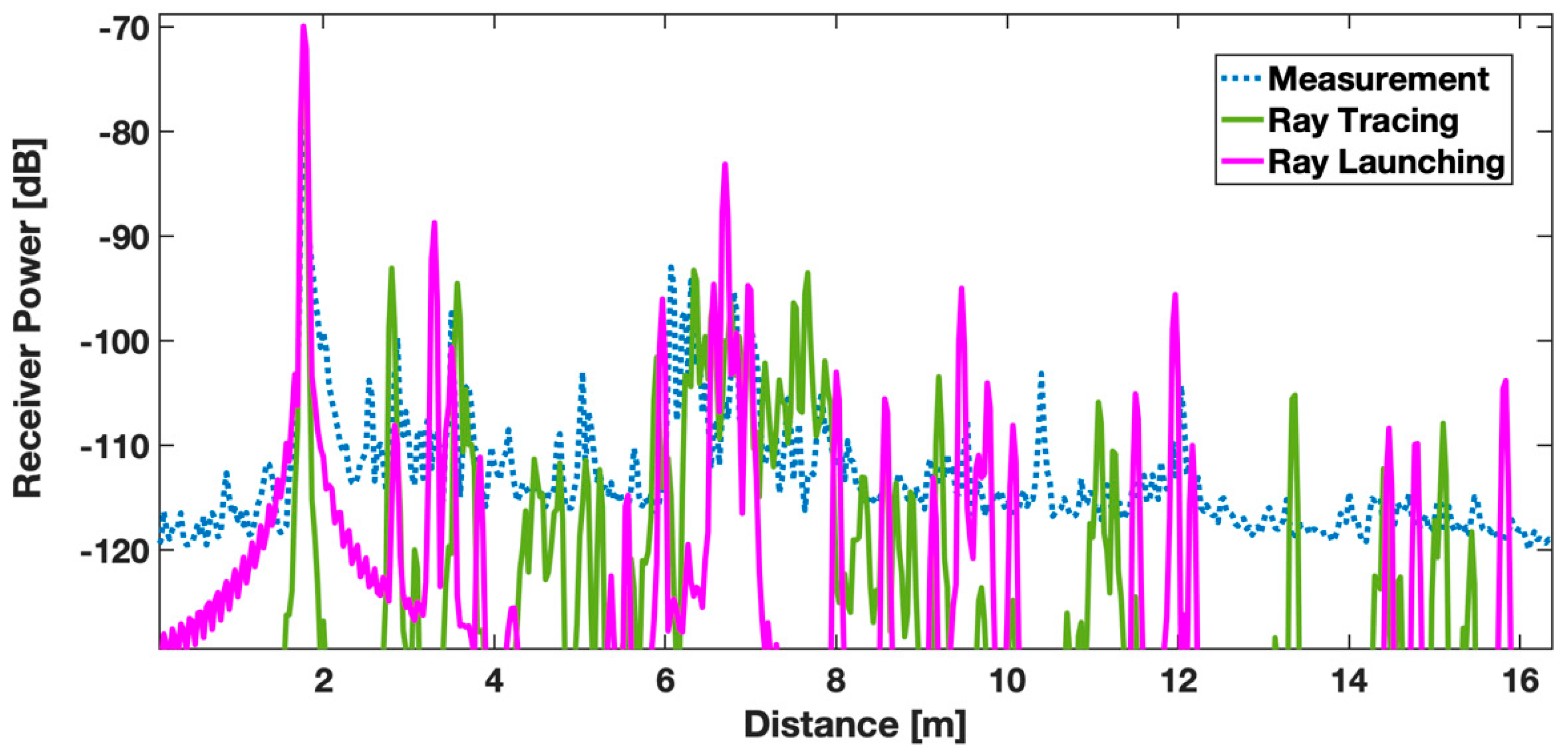
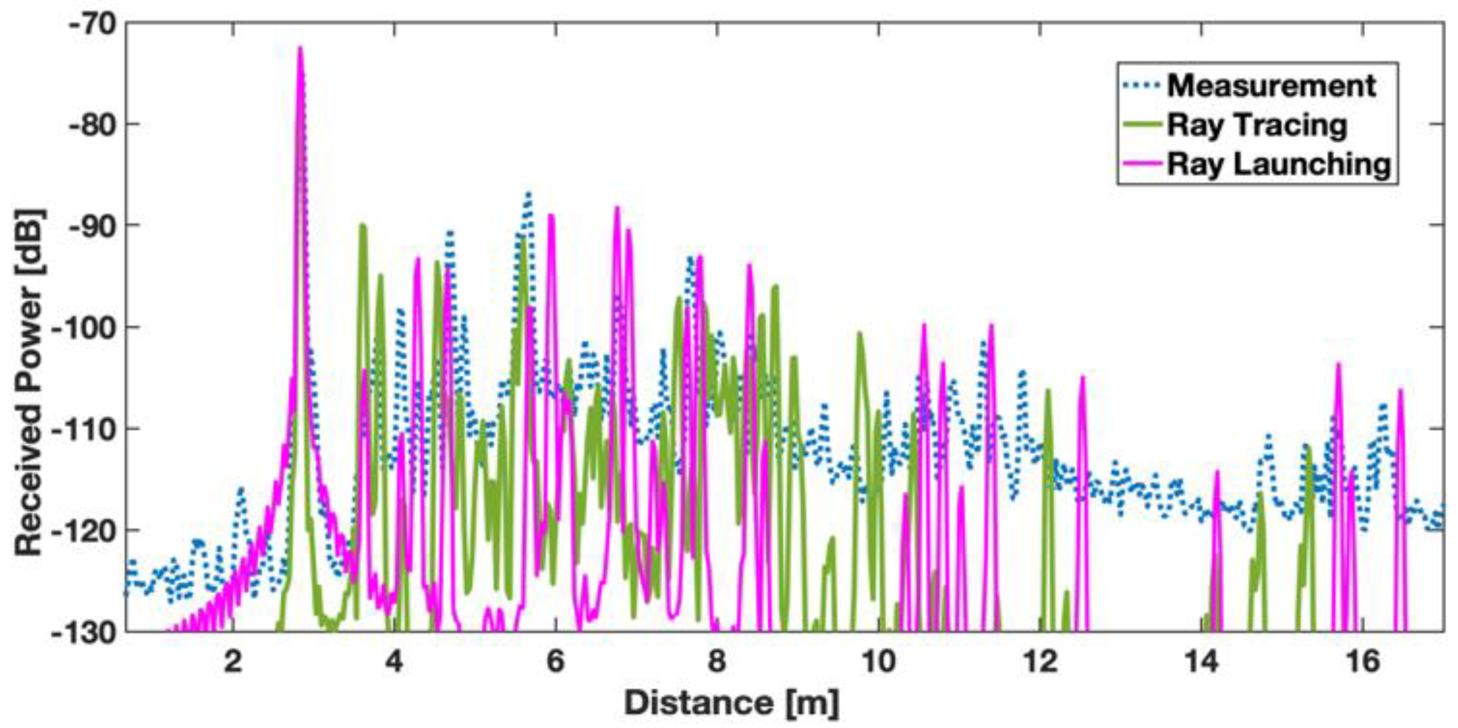
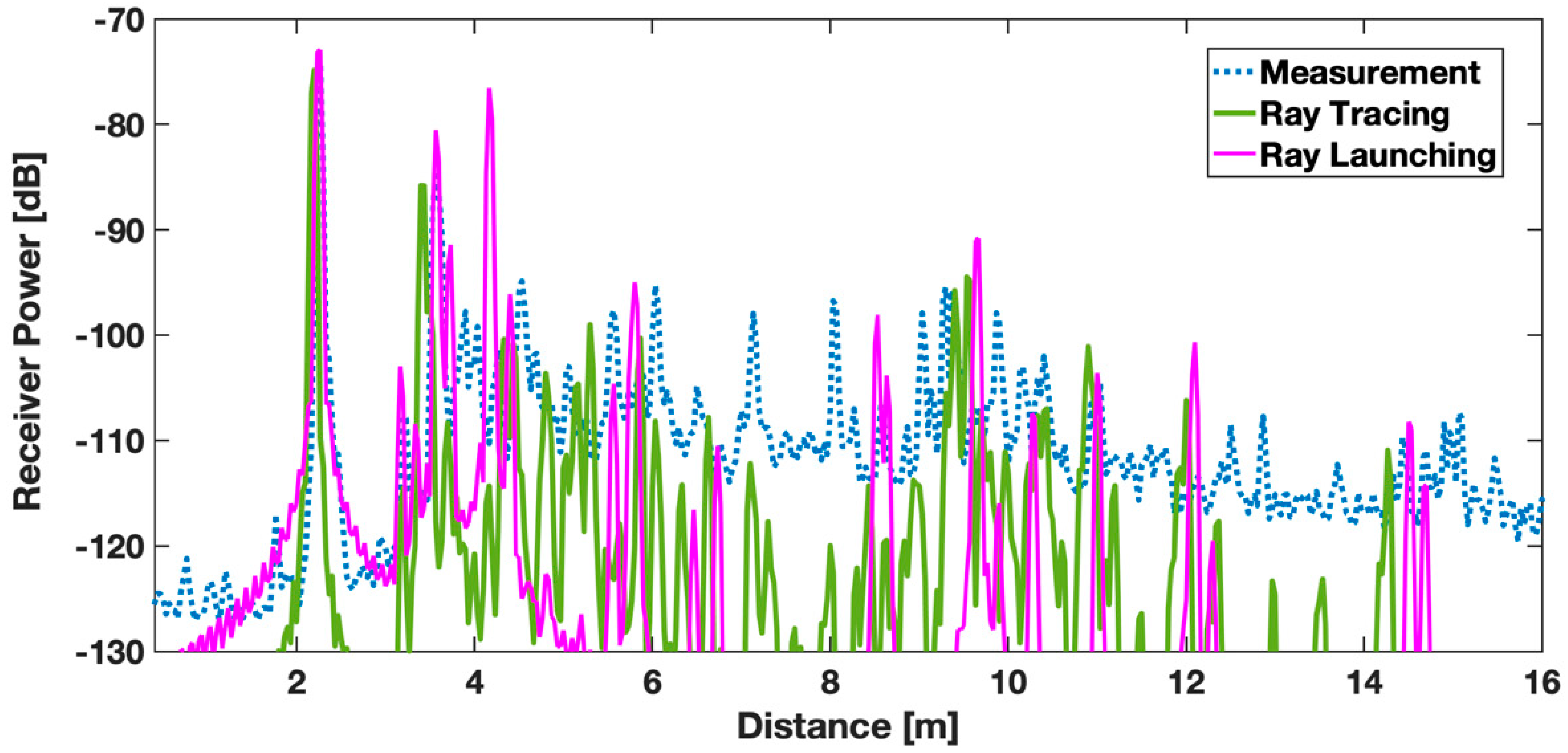
In programming using game engines, if the computer architecture offers multiple processors, it can allow the programmer to parallelize the game so that it can use all the resources and have improvements in performance. In Java, there is a Remote Method Invocation (RMI) to maximize the efficiency of multi-core processors. RMI allows the programmer to distribute the processes in which remote objects are invoked.

Multiple Java virtual machines (JVMs) were used on a single computer to parallelize the tasks and thus be able to use the multi-core processor as a system of distributed processes.

As a result of the pre-processing of rays, the list of stored candidate rays is taken and processed by the RMI server, executing a game engine for each nucleus and delivering a batch of candidate rays from the list. The RMI server stores in memory the list of the initial addresses of the rays to be launched from the transmitter, and then sends them sequentially and in order.

The game engine, upon receiving the address list of the rays to be launched from the transmitter, generates the rays with their initial parameters to be launched. Then it launches the generated rays into the environment, and they are processed in the GPU. In this stage, the GPU is efficiently used when processing a large number of rays in parallel and without displaying them on a monitor or screen. In the next rendering cycle, the GPU returns the list of processed rays to the CPU so that the game engine processes reception, reflection and diffraction, and generates the new list of rays to be launched in the next cycle. This process is repeated iteratively while the number of events is within the initial parameters.

The game engine receives from the graphics card a list of the rays that were processed by the GPU. The algorithm reads sequentially from the list of candidate rays, one by one, and identifies for each ray if it impacted with an object and determines the object with which it impacted (sphere, cylinder or plane). Depending on the impact object, it validates the impact and calculates its multipath parameters and verifies that the power level is above the threshold to continue or discard the ray.

In case of reflection or diffraction, it generates the new rays with their parameters to store them in a new list of rays to be launched from the impact position. Then it checks if there are more rays to be processed, and if it does, it reads the next ray in the list and processes it, otherwise, it ends the cycle for the rays sent by the GPU. Therefore, once all the rays are launched from a transmitter, it is possible to calculate the electric field at any reference point within the scenario.

3. Results

For this experiment, a maximum of two diffraction and a maximum of three consecutive interactions between reflections and diffraction were defined. The geometric separation resolution for the SBR is 0.13 as it is an indoor scenario and thus obtain a reasonable number of discrete rays in the analyzed scenario.

Figure 5 shows the result for the tracer, the launcher and the measurements for Position 3. In the graph you can see the differences between the two models and the measurements, being in this case very similar the results between the tracer and the launcher. The comparison has also been carried out quantitatively. Thus,

Table 2. Measured and simulated parameters.

	RMS [ns]
Position	Measure	Tracer	%	Launcher	%
3	4.22	4.41	95.5	3.92	92.9
7	3.77	3.52	93.4	4.05	92.57
18	4.32	3.70	83.2	3.81	88.2
	Medium Delay [ns]
Position	Measure	Tracer	%	Launcher	%
3	11.22	11.01	98.1	10.7	89
7	6.90	6.70	97.0	6.92	99.7
18	8.98	8.26	91.3	9.76	91.3
	PL [dB]
Position	Measure	Tracer	Dif.	Launcher	Dif.
3	71	74	3	69.7	1.3
7	72	70	2	67.2	4.8
18	71	72	1	67.88	2.12

shows the measured and estimated channel parameters; in particular, the mean square value of the delay (RMS), the average value of the delay (MD) and the basic propagation loss (PL) have been used.

In Figure 6 the results for Point 18 are shown, and, in this case, the result of the launcher is a little more like the real measurements than in the case of the tracer.

Statistics in Table 2 show very small differences between the two systems; the largest differences are found at Position 7 in which the ray tracer obtained a greater accuracy than the ray launcher in estimating the mean value while the launcher was more accurate in estimating the RMS. There are also some cases in which the percentage of accuracy is the same, for example, in the mean value of Position 18, and yet there is an appreciable difference between the results of both techniques.

Finally, comparison for Position 7 is observed in Figure 7; the accuracy is similar, although the tracer shows a group of replicas between 6 and 8 m that the launcher only partially represents. The precision is again similar without clearly distinguishing which of the two methods is more precise.

4. Discussion

The objective of programming the ray launcher in GPU-type processors is the acceleration of the estimation of the wireless channel. The ray launcher takes 36 h to estimate the path of all rays considered in the room. Once this simulation has been carried out, the 180 transfer functions in frequency for each channel can be obtained immediately and therefore the PDP for any position; so it can be said that the launcher takes 36 h to simulate the 20 measured locations, of which we have shown results for four of them. The ray tracing tool programmed in MATLAB takes around 13 h to simulate the 180 frequency transfer functions that allow finding the PDP of one position; that is, it is only necessary to perform the simulation of three locations to make the ray launcher programmed in the GPU profitable and therefore more computationally efficient with the same precision features.

The ray launcher is capable of including rays reflected of up to a third order; first order diffractions, up to two reflections after a diffraction, and up to two reflections with a subsequent diffraction. As seen in the results, this number of components is sufficient to accurately estimate the behavior of the wireless channel in the studied environment. A large number of contributions from the dispersers improve the electric fields received and, therefore, the prediction.

Next, another propagation environment is analyzed. High-density outdoor environments of buildings with low heights, determined by the downlink channel, predominantly reflected rays [24,25]. Diffraction components increase generating more rays. The combinations between reflection and diffraction events increase the number of rays and, therefore, the calculation time. However, there are external factors that decrease processing. Outdoors, the rays travel a greater distance, and this leads to only a few rays reaching the power above the sensitivity threshold of the receiver. Therefore, simulations in open environments can take the same time to interior simulations with good precision, such as that obtained in [26].

5. Conclusions

In this work, it has been shown that the programming of a ray launcher in GPU processors allows for the acceleration of the wireless channel estimation thanks to the parallelization of the ray-launching task. The accuracy of the launcher is high and has been compared with that achieved by a ray tracer. The differences between the simulations made with the ray launcher and the measurements may be due to the fact that, although the modeling of the environment was done more precisely in the launcher, there may be errors in locating objects of a few centimeters, which would affect the results at the frequencies used (millimeter waves). In future work the ray launcher will be compared with commercial ray launching tools to test their efficiency.

References

1. Calabuig, J.; Monserrat, J.F.; Gomez-Barquero, D. 5th Generation Mobile Networks: A New Opportunity for the Convergence of Mobile Broadband and Broadcast Services. IEEE Commun. Mag. 2015, 53, 198–205. [Google Scholar] [CrossRef]
2. Fettweis, G.; Alamouti, S. 5G: Personal mobile internet beyond what cellular did to telephony. IEEE Commun. Mag. 2014, 52, 140–145. [Google Scholar] [CrossRef]
3. International Wireless Industry Consortium (IWPC), Evolutionary & Disruptive Visions Towards Ultra High Capacity Networks. Available online:https://www.iwpc.org (accessed on 1 July 2019).
4. Gupta, A.; Jha, R.K. A Survey of 5G Network: Architecture and Emerging Technologies. IEEE Access 2015, 3, 1206–1232. [Google Scholar] [CrossRef]
5. Chandrasekhar, V.; Andrews, J.G.; Gatherer, A. Femtocell Networks: A Survey. IEEE Commun. Mag. 2008, 46, 59–67. [Google Scholar] [CrossRef]
6. Thompson, J.; Ge, X.; Wu, H.-C.; Irmer, R.; Jiang, H.; Fettweis, G.; Alamouti, S. 5G Wireless Communication Systems: Prospects and Challenges. IEEE Commun. Mag. 2014, 52, 62–64. [Google Scholar] [CrossRef]
7. Busari, S.A.; Mumtaz, S.; Al-Rubaye, S.; Rodríguez, J. 5G Millimeter-Wave Mobile Broadband: Performance and Challenges. IEEE Commun. Mag. 2018, 56, 137–143. [Google Scholar] [CrossRef]
8. Ni, Y.; Liang, J.; Shi, X.; Ban, D. Research on key technology in 5G mobile communication network. In Proceedings of the 2019 International Conference on Intelligent Transportation, Big Data & Smart City (ICITBS), Changsha, China, 12–13 January 2019. [Google Scholar]
9. Degli-Esposti, V. Ray Tracing propagation modelling: Future prospects. In Proceedings of the 8th European Conference on Antennas and Propagation (EuCAP 2014), The Hague, The Netherlands, 6–11 April 2014. [Google Scholar]
10. Rao, C.V.K.P. Signal modeling with stochastic and deterministic data: A lossless inverse scattering approach. In Proceedings of the ICASSP-88., International Conference on Acoustics, Speech, and Signal Processing, New York, NY, USA, 11–14 April 1988. [Google Scholar]
11. Key, C.; Troksa, B.; Kunkel, F.; Savic, S.V.; Ilic, M.M.; Notaros, B.M. Comparison of three sampling methods for shooting-bouncing ray tracing ssing a simple waveguide model. In Proceedings of the 2018 IEEE International Symposium on Antennas and Propagation & USNC/URSI National Radio Science Meeting, Boston, MA, USA, 8–13 July 2018. [Google Scholar]
12. Martinez-Ingle, M.-T.; Pascual-García, J.; Rodríguez, J.-V.; Molina-Garcia-Pardo, J.-M.; Juan-Llácer, L.; Gaillot, D.P.; Liénard, M.; Degauque, P. Indoor radio channel characterization at 60 GHz. In Proceedings of the 2013 7th European Conference on Antennas and Propagation (EuCAP), Gothenburg, Sweden, 8–12 April 2013. [Google Scholar]
13. Martinez-Ingles, M.-T.; Gaillot, D.P.; Pascual-Garcia, J.; Molina-Garcia-Pardo, J.-M.; Lienard, M.; Rodriguez, J.-V. Deterministic and Experimental Indoor mmW Channel Modeling. IEEE Antennas Wirel. Propag. Lett. 2014, 13, 1047–1050. [Google Scholar] [CrossRef]
14. Zhu, M.; Singh, A.; Tufvesson, F. Measurement based ray launching for analysis of outdoor propagation. In Proceedings of the 2012 6th European Conference on Antennas and Propagation (EUCAP), Prague, Czech Republic, 26–30 March 2012. [Google Scholar]
15. Lai, Z.; Bessis, N.; de LaRoche, G.; Song, H.; Zhang, J.; Clapworthy, G. An intelligent ray launching for urban prediction. In Proceedings of the 2009 3rd European Conference on Antennas and Propagation, Berlin, Germany, 23–27 March 2009. [Google Scholar]
16. Weng, J.; Tu, X.; Lai, Z.; Salous, S.; Zhang, J. Modelling the mmWave channel based on intelligent ray launching model. In Proceedings of the 2015 9th European Conference on Antennas and Propagation (EuCAP), Lisbon, Portugal, 13–17 April 2015. [Google Scholar]
17. Durgin, G.; Patwari, N.; Rappaport, T.S. An advanced 3D ray launching method for wireless propagation prediction. In Proceedings of the 1997 IEEE 47th Vehicular Technology Conference, Phoenix, AZ, USA, 4–7 May 1997. [Google Scholar]
18. Lu, W.; Chan, K. Advanced 3D Ray Tracing Method for Indoor Propagation Prediction. Electron. Lett. 1998, 34, 1259–1260. [Google Scholar] [CrossRef]
19. Navarro, A.; Guevara, D.; Gomez, J. A Proposal to Improve Ray Launching Techniques. IEEE Antennas Wirel. Propag. Lett. 2019, 18, 143–146. [Google Scholar] [CrossRef]
20. Liang, G.; Bertoni, H. A New Approach to 3-D Ray Tracing for Propagation Prediction in Cities. IEEE Trans. Antennas Propag. 1998, 46, 853–863. [Google Scholar] [CrossRef]
21. Navarro, A.; Guevara, D.; Cardona, N.; Gomez, J. Heuristic UTD Coefficients for Delay Spread Prediction in an Indoor Scenario. In Proceedings of the 11th European Conference on Antennas and Propagation (EUCAP), Paris, France, 19–24 March 2017. [Google Scholar]
22. Chen, S.-H.; Jeng, S.-K. An SBR/Image Approach for Radio Wave Propagation in Indoor Environments with Metallic Furniture. IEEE Trans. Antennas Propag. 1997, 45, 98–106. [Google Scholar] [CrossRef]
23. Yun, Z.; Iskander, M.F. Ray Tracing for Radio Propagation Modeling: Principles and Applications. IEEE Access 2015, 3, 1089–1100. [Google Scholar] [CrossRef]
24. Schneider, C.; Sommerkorn, G.; Narandzic, M.; Kaske, M.; Hong, A.; Algeier, V.; Kotterman, W.A.T.; Thoma, R.S.; Jandura, C. Multi-user MIMO channel reference data for channel modelling and system evaluation from measurements. In Proceedings of the 2009 International ITG Workshop on Smart Antennas, Berlin, Germany, 16–18 February 2009. [Google Scholar]
25. Rautiainen, T.; Wolfle, G.; Hoppe, R. Verifying path loss and delay spread predictions of a 3D ray tracing propagation model in urban environment. In Proceedings of the IEEE 56th Vehicular Technology Conference, Vancouver, BC, Canada, 24–28 September 2002. [Google Scholar]
26. Navarro, A.; Guevara, D.; Gomez, J. Prediction of delay spread using ray tracing and game engine based on measurement. In Proceedings of the 2015 IEEE 81st Vehicular Technology Conference (VTC Spring), Glasgow, UK, 11–14 May 2015. [Google Scholar]
Figure 1. 3D model of the laboratory.
Electronics 08 01121 g001
Figure 2. Top view of the electromagnetic characterization laboratory, Polytechnic University of Cartagena (UPCT), Spain. Distribution of measurement points.
Electronics 08 01121 g002
Figure 3. Measurement system for the measurement campaign between 57 and 66 GHz.
Electronics 08 01121 g003
Figure 4. Ray launching representation using the tube and icosahedron ray technique (left) and the cone beam technique.
Electronics 08 01121 g004
Figure 5. Comparison between the power delay profile (PDP) measured in Position 3, simulated with the tracer and simulated with the launcher programmed in the GPU.
Electronics 08 01121 g005
Figure 6. Comparison between the PDP measured at Position 18, simulated with the tracer and simulated with the launcher programmed in GPU.
Electronics 08 01121 g006
Figure 7. Comparison between the PDP measured at Position 7, simulated with the tracer and simulated with the launcher programmed in GPU.
Electronics 08 01121 g007