Bias Correction to Antenna Frequency Response for Wideband Polarimetric Phased Array Radar

Abstract

The frequency response of wideband polarimetric phased array radar antenna biases polarization measurement. A bias correction method named the iterative frequency division (IFD) algorithm is proposed in this paper to eliminate the effect of frequency response of the antenna system. The method is built on a new measurement bias model in which the effects of frequency response on the backscattering covariance matrix are analyzed. To demonstrate the effectiveness of the proposed method, a wideband microstrip patch array element is designed. Simulation results show that the biases of differential reflectivity ($Z_{DR}$) and linear depolarization ratio ($LDR$) can be decreased to less than $0.1$ dB and $-40\mathrm{dB}$ even for wide beam direction. The proposed method maintains a favorable polarization measurement accuracy for wideband polarimetric phased array radar.

1. Introduction

Recently, polarimetric phased array radar (PPAR) has attracted broad interest, owing to its potential in weather observation, air traffic control, and air surveillance [1,2,3,4,5,6,7]. However, some challenges, especially the requirement of high accuracy for polarimetric measurement, still hinder the development of the PPAR technology [7,8,9]. To be specific, the electric fields radiated from the horizontal (H) and vertical (V) ports are not orthogonal to each other caused by beam steering off the principal plane [3]. This leads to a cross-polar component where the polarization bias is generated. To address the problem, some calibration/correction methods have been studied. The bias correction technique for polarization measurement in PPAR was firstly put forward in [3], simulated in [9,10,11,12], and further updated in [13], and demonstrated in [5,14] using the large-scale testbeds. Thus far, most bias corrections focus on the narrow-band pulse. If the transmitted/received signal is wideband from a wideband polarimetric phased array radar (WPPAR), the pulse will be distorted due to the bandwidth effect of the antenna system [15]. The bias correction methods aforementioned cannot cover the wide bandwidth and inevitably cause the polarization measurement bias. Therefore, the wideband effect needs to be considered for accurate polarimetric measurement applications.

The wideband signal promises a higher resolution and detailed polarization profiles [15,16,17]. However, the frequency-dependent power amplifier (PA) and antenna system distort the output waveform in the WPPAR [18,19]. To circumvent the problem from PA, some digital pre-distortion schemes have been explored in [20,21,22,23]. Another challenge is from the transmitting/receiving antenna. The relative amplitude and phase of the far-field radiated by the wideband antenna are measured as a function of frequency and beam direction. The high fluctuation of amplitude and phase distort the wideband pulse [15,24]. Consequently, the distortion of received signals deteriorates the polarization measurement because the magnitude and phase of the signal lead to the bias of the scattering matrix. This is the problem we would like to address in this paper.

The polarimetric characteristic of the practical antenna varies with frequency, and the polarization non-orthogonality of H and V ports is also frequency-dependent. The polarimetric characteristic and polarization non-orthogonality are mutually coupled in the WPPAR. Hence, the frequency response of the wideband antenna is more complex for deteriorating the waveform fidelity for the transmitted/received pulse. In this paper, a polarization bias correction method named iterative frequency division (IFD) is proposed to address the above-mentioned coupled factors for the WPPAR. We analyze the process of transmission and reception of the pulse and derive the source of the polarization bias. The bias is reduced by a novel subband method involving the division of frequency band and the non-uniform selection of frequency point. The performance of the proposed method is verified by a designed wideband antenna element. Numerical simulations versus bandwidths and beam directions are investigated. The polarimetric variables, such as $Z_{DR}$ and $LDR$, are evaluated for the accurate polarization measurement.

The rest of the paper is organized as follows. In Section 2, the frequency response of the transmission process is deduced. In Section 3, the IFD algorithm for the wideband signal is provided to correct the scattering matrix. In Section 4, the polarimetric characteristics of the wideband microstrip antenna are analyzed, and the bias is quantified by the polarimetric variables. Simulation results and discussions are presented. Conclusions are presented in Section 5.

2. Theoretical Formulation of Bias

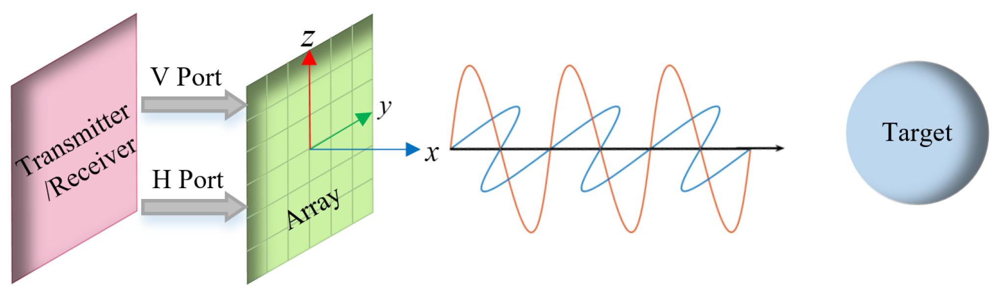
A typical signal transmission procedure between the antenna system and target, as illustrated in Figure 1, is considered. Horizontal (H) and Vertical (V) ports radiate and receive the individual electric field components. For the polarization measurement to a point target, the received voltage equation of the receiver can be expressed as [3,25]

$$\mathbf{V}={\mathbf{R}}^T·{\mathbf{S}}^{\left(\mathrm{b}\right)}·\mathbf{T},$$

(1)

where matrix $\mathbf{V}$ is the received open-circuit voltage. matrix $\mathbf{R}$ and matrix $\mathbf{T}$, describing the spacial polarization characteristics of the antenna, denote the transmitting pattern and receiving pattern, respectively. Generally, $\mathbf{R}$ is equal to $\mathbf{T}$ according to reciprocity principle. ${\mathbf{S}}^{\left(\mathrm{b}\right)}$ is the intrinsic backscatter matrix of the target. ${\mathbf{R}}^T$ is the transpose of $\mathbf{R}$. Rewriting Formula (1) in the form of a matrix gives

$$\left[\begin{array}{cc}{V}_{11}& V_{12}\\ V_{21}& V_{22}\end{array}\right]={\left[\begin{array}{cc}{R}_{11}& R_{12}\\ R_{21}& R_{22}\end{array}\right]}^T\left[\begin{array}{cc}{S}_{hh}^{\left(\mathrm{b}\right)}& S_{hv}^{\left(\mathrm{b}\right)}\\ S_{vh}^{\left(\mathrm{b}\right)}& S_{vv}^{\left(\mathrm{b}\right)}\end{array}\right]\left[\begin{array}{cc}{T}_{11}& T_{12}\\ T_{21}& T_{22}\end{array}\right].$$

(2)

Formula (2) can only be applied to the narrow-band signal or the situation where the bandwidth effect of the antennas is neglected. For the wideband case, the equation becomes

$$\mathbf{V}\left(f_R\right)=\frac{1}{f_R}{\mathbf{R}\left(f_R\right)}^T·{\mathbf{S}}^{\left(\mathrm{b}\right)}\left(f_R\right)·\mathbf{T}\left(f_R\right),$$

(3)

where $f_R$ is the radio frequency. The detailed derivation of Formula (2) is shown in Appendix A. For simplicity, the amplitude and phase imbalance of H and V channels, and the imperfect polarization isolation between H and V ports are neglected or idealized.

The voltage $\mathbf{V}\left(f_R\right)$ induced on the open-circuit terminal includes not only the scattering characteristic of the target but also the wideband properties of the transmitting and receiving antennas. It is frequency-dependent. We describe the characteristics of an antenna as a system transfer function mathematically, assuming that ${\mathbf{S}}^{\left(\mathrm{b}\right)}\left(f_R\right)$ is constant. Given that the amplitudes of the transmitted signals are unit amplitudes and the relative phases are 0°, $\mathbf{V}\left(f_R\right)$ represents the amplitude and phase modulations to the signal’s spectrum with the input frequency. The waveform information is carried by the emission pulse and is not related to $\mathbf{V}\left(f_R\right)$. Thus, it can be seen that the waveform of the received signals is modulated in the frequency domain. For each channel, $V\left(f_R\right)$ is a complex number and denotes the relation between the source and received signal. The relation is expressed as follows:

$${\overline{X}}_r\left(f_R\right)=V\left(f_R\right)·{\overline{X}}_i\left(f_R\right),$$

(4)

where ${\overline{X}}_r\left(f_R\right)$ is the output signal of the receiving antenna and ${\overline{X}}_i\left(f_R\right)$ is the spectrum of the input signal $\overline{x}\left(t\right)$. The overbar on symbol denotes that the signal is on a carrier, i.e., it has not yet been demodulated.

It is worth mentioning that the transmitted/received signal should be amplified in practical radar systems by the high power amplifier (HPA) in transmitting antenna and the low noise amplifier (LNA) in receiving antenna. The nonlinear behavior of the amplifier introduces distortion in the output pulse. Dunn et al. used the digital pre-distortion technique to minimize the distortion of amplified signals that appear to be linearly amplified [20,21,22,23]. With the linear assumption on the amplifier in the WPPAR system, this paper focuses on the frequency response of the antenna systems.

When the antenna system operates in the alternate transmission and simultaneous reception (ATSR) mode, all four components of the backscattering covariance matrix can be estimated from two or more pulses. Hence, the received signals can be expressed as

$$\left[\begin{array}{cc}{\overline{X}}_{r11}\left(f_R\right)& {\overline{X}}_{r12}\left(f_R\right)\\ {\overline{X}}_{r21}\left(f_R\right)& {\overline{X}}_{r22}\left(f_R\right)\end{array}\right]=\left[\begin{array}{cc}{V}_{11}\left(f_R\right)& V_{12}\left(f_R\right)\\ V_{21}\left(f_R\right)& V_{22}\left(f_R\right)\end{array}\right]·{\overline{X}}_i\left(f_R\right).$$

(5)

For simplicity, Equation (5) is rewritten as

$${\overline{\mathbf{X}}}_r\left(f_R\right)=\mathbf{V}\left(f_R\right)·{\overline{X}}_i\left(f_R\right).$$

(6)

It can be seen that the waveforms of received signals in four channels are modulated by transfer function $\mathbf{V}\left(f_R\right)$ in the frequency domain. The transfer function is determined by the impedance matching, gain, polarization matching et al. of the transmitting/receiving antenna.

The signal representations in the time and frequency domain are symmetrical. To facilitate the following derivation, the measurement bias is conducted in the frequency domain. In addition, the internal thermal noise and the external environmental noise are ignored herein. In a modern radar system, the carrier frequency of the received signal should be removed firstly [26], and the echo signal after downconversion is referred to as a baseband signal. The spectra of the baseband signals in matrix form can be written as

$${\mathbf{X}}_r\left(f\right)=\mathbf{V}\left(f_R\right)·X_i\left(f\right),$$

(7)

where f is the frequency of the baseband signal.

The four signals are sent to matched filters in the frequency domain, and the outputs of four channels from the matched filters are

$$\begin{array}{cc}\hfill {\mathbf{X}}_m\left(f\right)& ={\mathbf{X}}_r\left(f\right)·{X_i}^{*}\left(f\right)\hfill \\ & =\mathbf{V}\left(f_R\right)·X_i\left(f\right)·{X_i}^{*}\left(f\right)\hfill \\ & =\mathbf{V}\left(f_R\right)·{\left|X_i\left(f\right)\right|}^2,\hfill \end{array}$$

(8)

where $X^{*}\left(f\right)$ is the impulse response of matched filters.

The output of the matched filter in the time domain is

$${\mathbf{o}}^{\left(\mathrm{p}\right)}\left(t\right)=\left[\begin{array}{cc}{o}_{11}^{\left(\mathrm{p}\right)}\left(t\right)& o_{12}^{\left(\mathrm{p}\right)}\left(t\right)\\ o_{21}^{\left(\mathrm{p}\right)}\left(t\right)& o_{22}^{\left(\mathrm{p}\right)}\left(t\right)\end{array}\right]=\mathrm{IFT}\left({\mathbf{X}}_m\left(f\right)\right),$$

(9)

where $IFT\left(\right)$ denotes the Inverse Fourier Transform.

It is clear in Equation (9) that both the amplitude and phase of four output signals are modulated by the complex matrix through the transmitting, scattering and receiving process. The modulation finally results in the distortion of echo signals, thereby deteriorating the measurement accuracy of the backscattering matrix. The maximum values of the filters’ output are obtained and the measured scattering matrix can be expressed as

$${\mathbf{S}}^{\left(\mathrm{p}\right)}=\left[\begin{array}{cc}{S}_{hh}^{\left(\mathrm{p}\right)}& S_{hv}^{\left(\mathrm{p}\right)}\\ S_{vh}^{\left(\mathrm{p}\right)}& S_{vv}^{\left(\mathrm{p}\right)}\end{array}\right],$$

(10)

where $S_{\mathrm{ij}}^{\left(\mathrm{p}\right)}$ denotes the peak value of $o_{\mathrm{ij}}^{\left(\mathrm{p}\right)}\left(t\right)$, $\mathrm{i},\mathrm{j}=h$ or v.

If the projection matrix method in [3] is utilized to correct the measured scattering matrix, only one frequency point is considered for correction. For example, the projection matrix corresponding to the center frequency $f_0$ is selected as the correction matrix, and the expression is written as

$$\widehat{\mathbf{S}}\left(f_0\right)={\mathbf{C}}^T\left(f_0\right)·{\mathbf{S}}^{\left(\mathrm{p}\right)}·\mathbf{C}\left(f_0\right),$$

(11)

where $\mathbf{C}$ is the correction matrix, $\mathbf{C}={\mathbf{T}}^{-1}$.

In fact, the correction matrix $\mathbf{C}$ involves the polarization characteristics including the cross-polar, polarization non-orthogonality. For the narrow-band case, $\mathbf{C}$ is related to the beam direction. However, for the wideband case, $\mathbf{C}$ is related to the frequency as well and can be denoted as $\mathbf{C}\left(f_R\right)$. Therefore, Equation (11) should be rewritten for the wideband antenna as

$$\widehat{\mathbf{S}}\left(f_R\right)={\mathbf{C}}^T\left(f_R\right)·{\mathbf{S}}^{\left(\mathrm{p}\right)}·\mathbf{C}\left(f_R\right).$$

(12)

Theoretically, each frequency point corresponds to one correction matrix, and each correction matrix corresponds to one corrected scattering matrix. The bias of polarization measurement varies with the input frequency, so we should select the frequency point that could minimize the correction bias. However, this expected frequency point that could satisfy the accurate polarization measurement does not necessarily exist because the selection of the correction matrix is related to the smoothness of the system transfer function $\mathbf{V}\left(f_R\right)$. Therefore, a bias correction method for the wideband case is proposed in this paper for the accuracy requirement of polarization measurement for WPPAR.

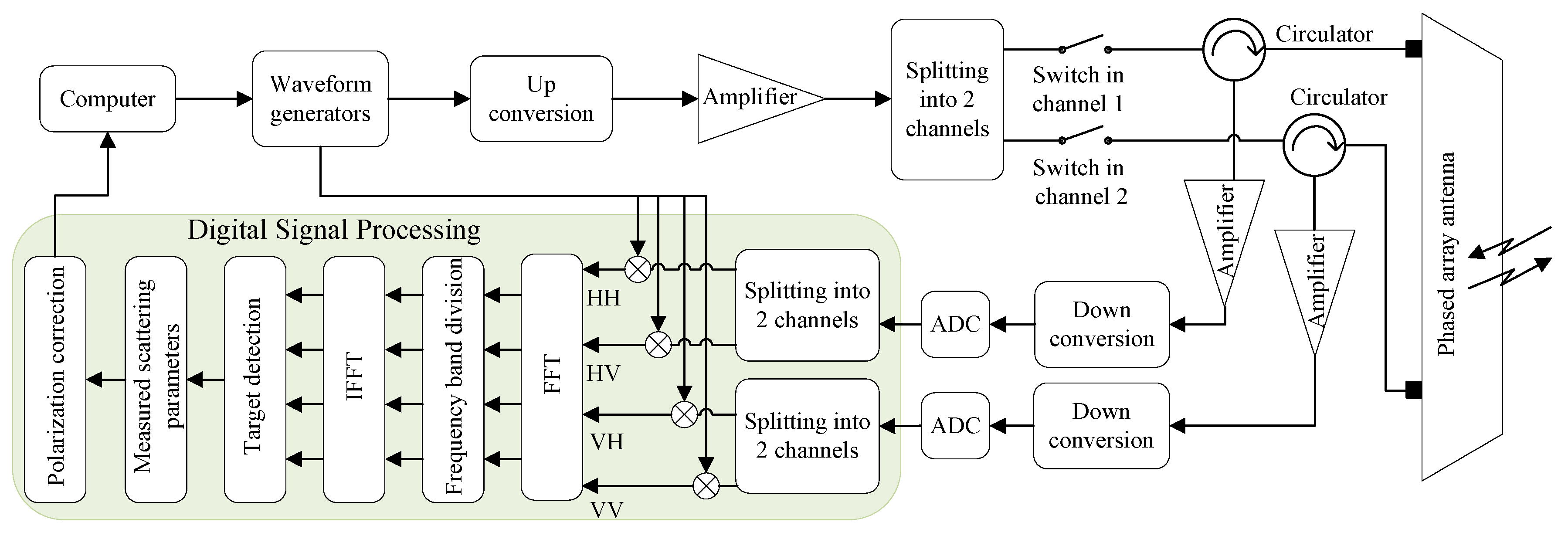
3. Correction Algorithm

The scheme of bias correction for the frequency response is displayed in Figure 2. The correction is implemented in the digital domain (the coloring regions in Figure 2). The correction matrix $\mathbf{C}\left(f_R\right)$ is frequency-dependent and is diverse from each frequency point. To reduce the number of frequency points, the correction can be done by using some specific points in the corresponding subbands, namely the frequency band division method. The measured scattering matrix ${\mathbf{S}}^{\left(\mathrm{p}\right)}$ is corrected by the correction matrices corresponding to each given subband. The sum of the estimated values is taken as the correction result. This method will improve correction effectiveness and maintain the polarization measurement accuracy.

The output of the matched filter in the frequency domain is denoted as ${\mathbf{X}}_m\left[k\right]$ in the digital signal processing, where $k=1,2,\cdots ,K$, K is the total number of sampling points in the frequency band. We divide the bandwidth (specifically, 3 dB bandwidth herein) of ${\mathbf{X}}_m\left[k\right]$ to multiple subbands. To be specific, the emphasis is on how to divide the frequency into subband and how to select one frequency point in each subband to obtain the corresponding correction matrix. The frequency point in each subband is selected to obtain the minimal estimation bias. Therefore, the problem in this paper can be described as a frequency point selection problem. 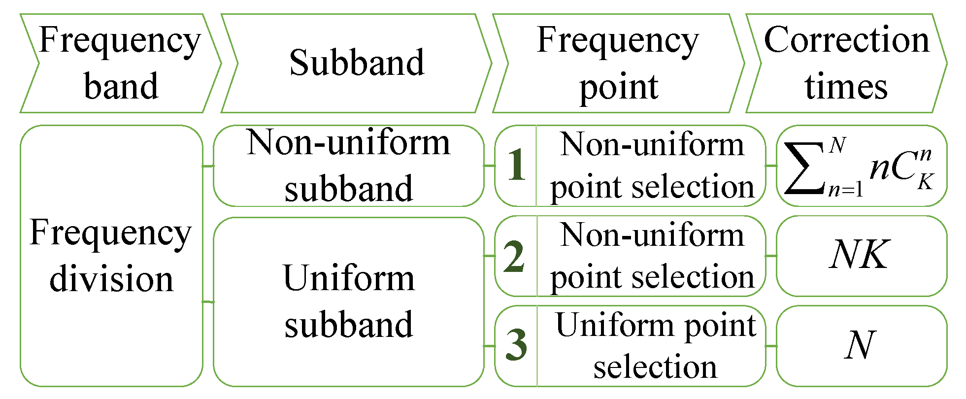The number of the selected frequency points is defined as N, the same as the number of subbands. The frequency division strategies and their computational complexity are shown in Figure 3. Several alternative ways are available.

• Strategy 1: Selecting the non-uniform frequency point in the individual non-uniform subband is equivalent to selecting the frequency point randomly. The number of permutation and combination for selecting n frequency points in K sampling points is $C_K^n$. To compare the effectiveness of the various permutation of the frequency point selection, the correction to the scattering matrix is implemented for each permutation. Thus, the correction times for n frequency points is $n{C}_K^n$. To obtain N optimal frequency points iteratively, the total correction times is ${\sum }_{n=1}^{N}n{C}_K^n$. The computation complexity has an exponential growth with the increasing number of frequency points.
• Strategy 2: If the non-uniform point is selected in the individual uniform subband, the correction times $K_n$, that is, the sampling points in each subband is $K/N$. The correction times in the total frequency band remains unchanged with N and is K. The total correction times is $NK$ before the iteration operation is completed. Obviously, the computation complexity of this strategy is considerably lower than that of Strategy 1. If the frequency response does not fluctuate dramatically, the way dividing the transfer function $\mathbf{V}\left[k\right]$ uniformly with an equal bandwidth interval is reasonable.
• Strategy 3: Uniform point selection in the uniform subband describes the case that the frequency point position is invariant for each subband, such as the center frequency. The strategy has fewer correction times. However, the frequency point is not necessarily optimal in each subband, and the number of needed frequency points will be greater than the two strategies mentioned above.

${\mathbf{X}}_{mn}\left[k\right]$ represents the nth subband of the matched filter output. According to Equations (8)–(10), the measured scattering matrix ${\mathbf{S}}_n^{\left(\mathrm{p}\right)}$ of the nth subband can be derived. When the correction is done within the subband, the estimated scattering matrix is given by

$${\widehat{\mathbf{S}}}_n\left[k\right]={\mathbf{C}}_n^T\left[k\right]·{\mathbf{S}}_n^{\left(\mathrm{p}\right)}·{\mathbf{C}}_n\left[k\right],$$

(13)

where ${\mathbf{C}}_n\left[k\right]$ denotes the kth correction matrix for the nth subband, corresponding to the k frequency point.

Now, the problem has become a choice matter of the frequency point, thereby obtaining the global optimal correction matrix. The iteration calculation is a candidate as a way to get the optimal results mathematically. If the frequency is divided iteratively, the number of subbands increases gradually and the number of frequency points has a continuous increase. The operation is repeated until the bias is corrected acceptably. The method is referred to as the iterative frequency division (IFD) algorithm. Using the IFD method, the bias of ${\widehat{\mathbf{S}}}_n\left[k\right]$ could be as low as possible. The formula in (13) is expanded for analyzing the polarization bias as follows:

$${\widehat{\mathbf{S}}}_n\left[k\right]={\left[\begin{array}{cc}{C}_{n11}\left[k\right]& C_{n12}\left[k\right]\\ C_{n21}\left[k\right]& C_{n22}\left[k\right]\end{array}\right]}^T\left[\begin{array}{cc}{S}_{nhh}^{\left(\mathrm{p}\right)}& S_{nhv}^{\left(\mathrm{p}\right)}\\ S_{nvh}^{\left(\mathrm{p}\right)}& S_{nvv}^{\left(\mathrm{p}\right)}\end{array}\right]\left[\begin{array}{cc}{C}_{n11}\left[k\right]& C_{n12}\left[k\right]\\ C_{n21}\left[k\right]& C_{n22}\left[k\right]\end{array}\right].$$

(14)

In addition, the four elements of the corrected scattering matrix are written as

$$\left\{\begin{array}{cc}\hfill & {\widehat{S}}_{nhh}\left[k\right]=C_{n11}^2\left[k\right]S_{nhh}^{\left(\mathrm{p}\right)}+C_{n21}\left[k\right]C_{n11}\left[k\right]S_{nvh}^{\left(\mathrm{p}\right)}+C_{n11}\left[k\right]C_{n21}\left[k\right]S_{nhv}^{\left(\mathrm{p}\right)}+C_{n21}^2\left[k\right]S_{nvv}^{\left(\mathrm{p}\right)},\hfill \\ \hfill & {\widehat{S}}_{nhv}\left[k\right]=C_{n11}\left[k\right]C_{n12}\left[k\right]S_{nhh}^{\left(\mathrm{p}\right)}+C_{n21}\left[k\right]C_{n12}\left[k\right]S_{nvh}^{\left(\mathrm{p}\right)}+C_{n11}\left[k\right]C_{n22}\left[k\right]S_{nhv}^{\left(\mathrm{p}\right)}+C_{n21}\left[k\right]C_{n22}\left[k\right]S_{nvv}^{\left(\mathrm{p}\right)},\hfill \\ \hfill & {\widehat{S}}_{nvh}\left[k\right]=C_{n12}\left[k\right]C_{n11}\left[k\right]S_{nhh}^{\left(\mathrm{p}\right)}+C_{n11}\left[k\right]C_{n22}\left[k\right]S_{nvh}^{\left(\mathrm{p}\right)}+C_{n12}\left[k\right]C_{n21}\left[k\right]S_{nhv}^{\left(\mathrm{p}\right)}+C_{n21}\left[k\right]C_{n22}\left[k\right]S_{nvv}^{\left(\mathrm{p}\right)},\hfill \\ \hfill & {\widehat{S}}_{nvv}\left[k\right]=C_{n12}^2\left[k\right]S_{nhh}^{\left(\mathrm{p}\right)}+C_{n12}\left[k\right]C_{n22}\left[k\right]S_{nvh}^{\left(\mathrm{p}\right)}+C_{n22}\left[k\right]C_{n12}\left[k\right]S_{nhv}^{\left(\mathrm{p}\right)}+C_{n22}^2\left[k\right]S_{nvv}^{\left(\mathrm{p}\right)}.\hfill \end{array}\right.$$

(15)

The sum of N corrected matrices is referred to as the scattering matrix of the wideband polarization measurement,

$$\widehat{\mathbf{S}}=\sum _{n=1}^N{\widehat{\mathbf{S}}}_n,$$

(16)

where ${\widehat{\mathbf{S}}}_n=\left[\begin{array}{cc}{\widehat{S}}_{nhh}& {\widehat{S}}_{nhv}\\ {\widehat{S}}_{nvh}& {\widehat{S}}_{nvv}\end{array}\right]$.

Therefore, the estimated polarization scattering matrix (PSM) of the observed target can be computed.

To evaluate the performance of the correction matrix for polarization bias correction, we use the polarimetric variables including the differential reflectivity ($Z_{DR}$) and linear depolarization ratio ($LDR$) [25]. The scattering phenomenon is modeled as a reflection from a single point scatterer. The echo signal is received after the two-way propagations, that is, before and after scattering. The scattering matrix can be estimated through the echo by using correction methods, and the corrected ${\widehat{Z}}_{DR}$ scaled in dB is given by

$${\widehat{Z}}_{DR}=10\log \left(\frac{{\left|{\widehat{S}}_{hh}\right|}^2}{{\left|{\widehat{S}}_{vv}\right|}^2}\right).$$

(17)

We describe the bias of differential reflectivity with

$$\Delta Z_{DR}=\left|{\widehat{Z}}_{DR}-Z_{DR}\right|.$$

(18)

The expected requirement for $\Delta Z_{DR}$ is less than $0.1$ dB for the phased array radar system [14]. The scattering matrix of the target in this research is a unit matrix. Thus, $S_{hh}=S_{vv}$ and $Z_{DR}=0$. Hence, the bias of differential reflectivity is equal to the differential reflectivity after correcting, namely, $\Delta Z_{DR}={\widehat{Z}}_{DR}$.

Consider the assumption that the intrinsic scattering matrix of the target is a unit matrix, namely, $S_{hv}=S_{vh}=0$, the measured $\widehat{LDR}$ is strictly the bias of $LDR$. Hence, the $\Delta LDR$ of H channel after correcting scaled in dB is given by

$$\Delta LD{R}_h={\widehat{LDR}}_h=10\log \left(\frac{{\left|{\widehat{S}}_{vh}\right|}^2}{{\left|{\widehat{S}}_{hh}\right|}^2}\right).$$

(19)

We assume that the constraint condition of the polarization variable measurement is $\Delta LD{R}_h\le -40\mathrm{dB}$.

Two constraint conditions are utilized to determine how many subbands it needs to be divided into, and the two polarization variables imply the relative relations of four components in the scattering matrix. To increase the data comparability, we normalize the $\Delta Z_{DR}$ and $\Delta LD{R}_h$, and the sum of normalized data $\Delta Z_{DR}^{nor}$ and $\Delta LD{R}_h^{nor}$ is written as

$$\delta =\Delta Z_{DR}^{nor}+\Delta LD{R}_h^{nor}.$$

(20)

The framework of the IFD algorithm for bias correction is displayed in Algorithm 1.

Algorithm 1: IFD for bias correction

The input of the algorithm is the matched filter output ${\mathbf{X}}_m\left[k\right]$, system transfer function $\mathbf{V}\left[k\right]$. The output of the algorithm is the minimal number of the subbands N. The iterative operations start with n = 1. Firstly, we divide ${\mathbf{X}}_m\left[k\right]$ to N sections uniformly, such as ${\mathbf{X}}_{m1}\left[k\right],{\mathbf{X}}_{m2}\left[k\right],\cdots ,{\mathbf{X}}_{mN}\left[k\right]$. Secondly, a time-frequency conversion is made for the nth subband ${\mathbf{X}}_{mn}\left[k\right]$ by using the IFT. The scattering matrix ${\mathbf{S}}_n^{\left(\mathrm{p}\right)}$ can be measured through detecting the peak value. Thirdly, ${\mathbf{S}}_n^{\left(\mathrm{p}\right)}$ is corrected by multiplying the correction matrices corresponding to $K_n$ frequency points in the current subband. We select the frequency point which could minimize the $\delta$ as the expected one, and take the N corrected results as the total corrected results. Lastly, N increases progressively and repeats the operations above until $\Delta Z_{DR}\le 0.1$ dB and $\Delta LD{R}_h\le -40$ dB. Therefore, the corrected $\widehat{S}$ of the observed target is computed and the number N of the subbands is determined.

4. Simulation Results and Analyses

In this section, we provide the polarimetric characteristics with the frequency and off-axis deviation angle based on a designed wideband polarimetric antenna. The numerical results and comparisons present the correction to the polarization measurement bias. Furthermore, the reasons for the number of frequency points selection are discussed.

4.1. The Polarization Characteristics of a Wideband Polarimetric Antenna

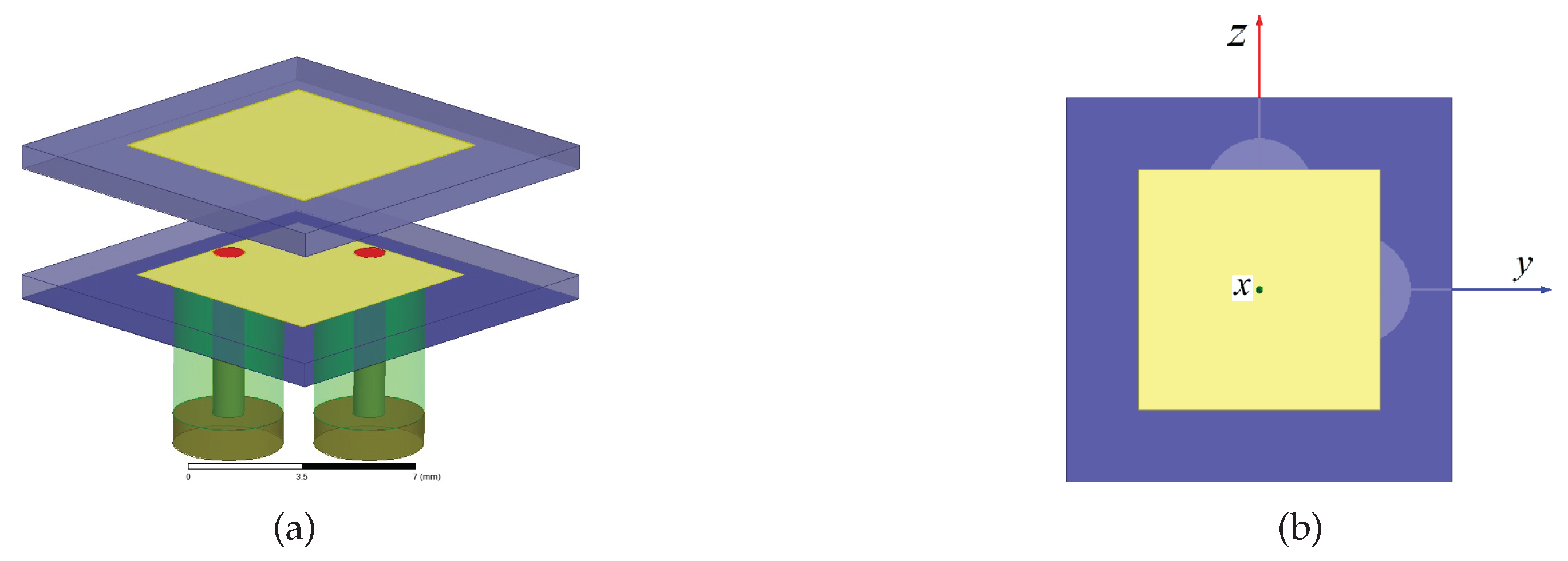
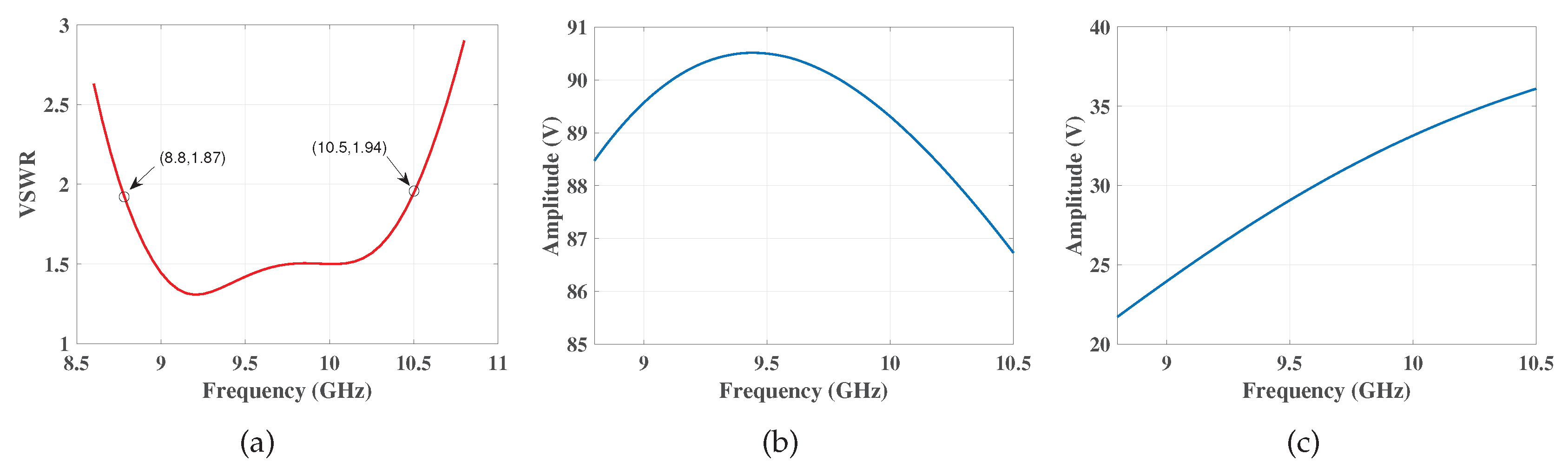
A wideband microstrip patch antenna is designed by High Frequency Structure Simulator (HFSS) software to demonstrate the frequency response. The design of this wideband antenna is relatively mature and applied abroad, and its radiation characteristics can be used to test the influence of frequency response on polarization measurement. This is an X-band microstrip patch antenna which adopts two layers of substrates. The dielectric constant of the substrates ${ϵ}_r=4.3$, and the medium between the upper substrate and the lower substrate is air. The feeding configuration is a coaxial probe as displayed in Figure 4. Considering the antenna’s voltage standing wave ratio (VSWR), as shown in Figure 5a, the bandwidth is up to $1.77$ GHz when VSWR $\le 2$.

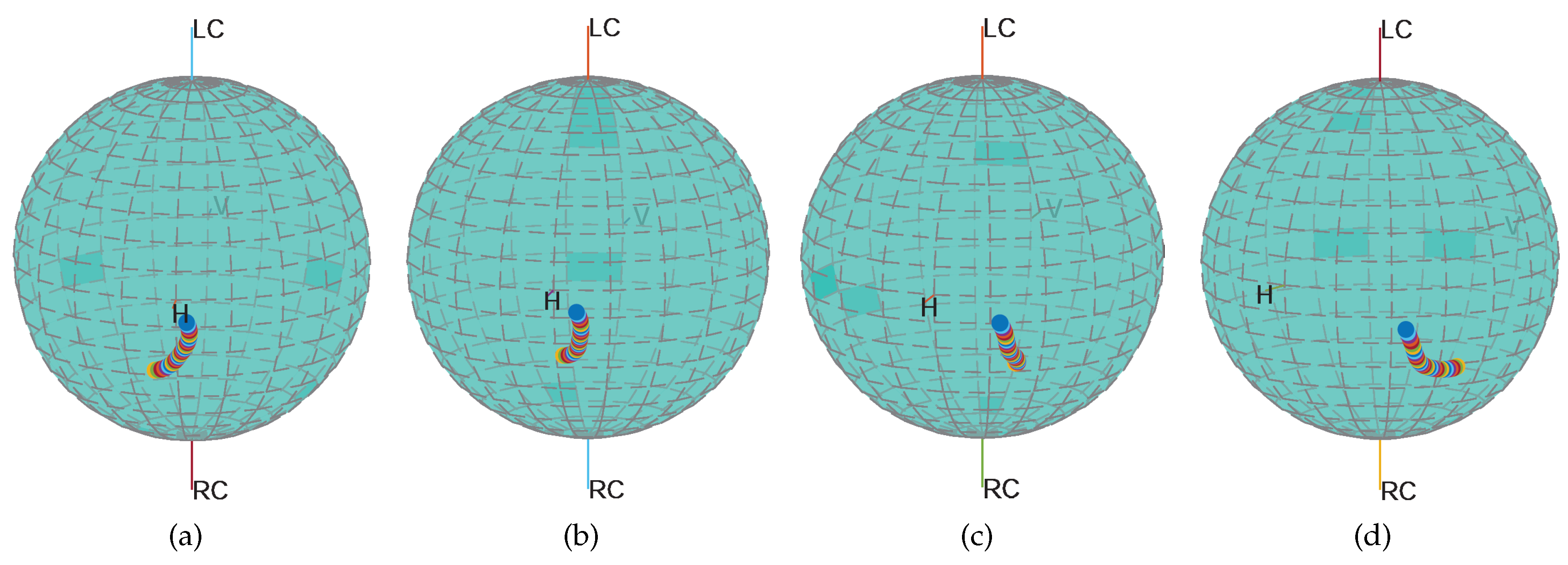
The electric fields of H and V ports create cross-polar coupling (i.e., polarization non-orthogonality) when the beam direction is away from the broadside (x-axis) of the antenna array. The off-axis deviation angle, the beam deviating from the boresight direction, is indicated with ($\varphi ,\theta$). $\varphi$ is the azimuth angle. $\theta$ is the angle subtended from the z-axis. Without loss of generality, we choose ($\varphi ,\theta$) in the three-dimensional space and assume that a complementary angle relationship is restrained between $\varphi$ and $\theta$, which is $\varphi +\theta =\frac{\pi }{2}$.

We use HFSS to compute the radiation fields ${\mathbf{E}}_{\varphi }$ and ${\mathbf{E}}_{\theta }$ from the H and V ports which are activated alternately. Figure 6 shows the polarization state of the radiated fields from the H port. The points distribution on the Poincare sphere describes the variation of the polarization state. The investigation has manifested that polarization state changes with the bandwidth, that is, the amplitude of ${\mathbf{E}}_{\varphi }$ and ${\mathbf{E}}_{\theta }$ is not invariable or flat and the phase of ${\mathbf{E}}_{\varphi }$ and ${\mathbf{E}}_{\theta }$ is not linear. Meanwhile, the state changes across with the deviation angle.

The polarization state of fields from V port is similar to that of the H port. In addition to the variation of the polarization state in each frequency point, the non-orthogonality state of fields from H and V ports also changes over the bandwidth and beam direction separately. The intercoupling between the polarization state and the non-orthogonality makes it more complicated in the bias terms, and both of them contribute to the frequency response. In fact, the transmitting and receiving process all have the frequency response, so it will affect the measurement twice. The influence of the complex polarization characteristics on the polarization measurement accuracy is investigated in the next subsection.

4.2. Bias Correction with Bandwidth and Deviation Angle

The simulations and tests are conducted on the array antenna element and the tests are carried out in the ATSR mode. The emission waveform is the linear frequency modulation (LFM) signal and the central frequency is $9.5$ GHz. The bandwidth B increases gradually from 100 MHz to 1700 MHz with a 100 MHz interval, and the pulse duration $\tau$ from $1\mathsf{\mu }\mathrm{s}$ to $17\mathsf{\mu }\mathrm{s}$ with $1\mathsf{\mu }\mathrm{s}$ interval. The chirp rate $B/\tau$ remains invariant, so the waveforms are consistent for pulses with different bandwidths. The trends of the $\Delta Z_{DR}$ and $\Delta LD{R}_h$ are investigated based on different bandwidths and beam directions.

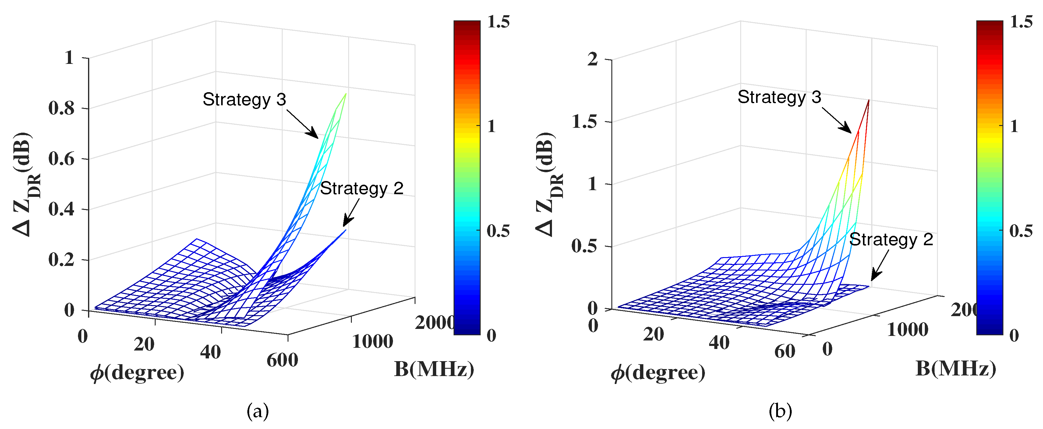
To manifest that the superiority of the non-uniform frequency point selection in the subband (Strategy 2)is better than the uniform selection (Strategy 3), a comparison is conducted. Situations when $n=1$ and $n=2$ are presented in Figure 7. The upper mesh surface in Figure 7a describes the bias after polarization correction using Strategy 3 across with the bandwidth B and deviation angle $\varphi$, and the lower mesh surface using Strategy 2. It can be seen that the polarization variable $\Delta Z_{DR}$ is lower when the frequency point selection is optimized. Similar results have been observed when $N=2$, as illustrated in Figure 7b. It is worth noting that Strategy 3 when $N=2$ does not result in lower correction bias than that when $N=1$, so the effect of Strategy 3 is doubtful. However, Strategy 2 can reduce the $\Delta Z_{DR}$ considerably. In addition to $\Delta Z_{DR}$, a similar situation exists for $\Delta LD{R}_h$ and differential phase (${\Phi }_{\mathrm{DP}}$). Therefore, it is essential to search the optimal frequency point, thereby obtaining the corresponding correction matrix. Thus, the polarization measurement bias could be reduced. In the following analysis and discussion, only Strategy 2 is considered.

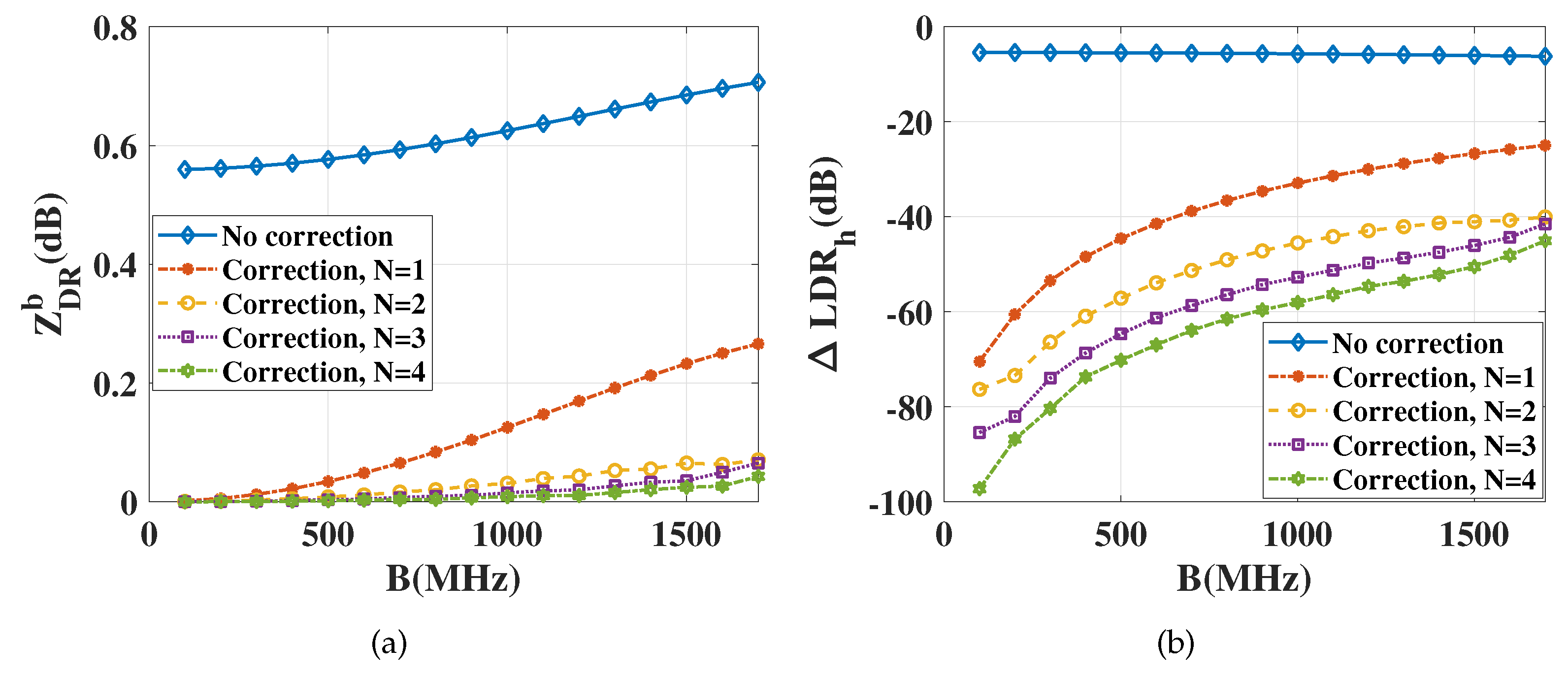
Comparison of the corrected results for different N is displayed in Figure 8. Figure 8a shows that the measured $\Delta Z_{DR}$ is $0.56$ dB greater than that when the system frequency response acts on the polarization scattering matrix without correction. When N = 1, namely a single matrix corresponding to a single frequency point is used for correction, the biases decrease significantly. When N is larger than 2, the change is slight. However, the biases increase gradually with the gain of bandwidth, which proves the effect of bandwidth on the polarimetric measurement accuracy. Similarly, the $\Delta LD{R}_h$ in Figure 8b increases with bandwidth. As manifested in Figure 8, the corrected $\Delta Z_{DR}$ is less than $0.1$ dB over the whole bandwidth if $N\ge 2$, and $\Delta LD{R}_h$ is less than $-40$ dB when the bandwidth is up to 1700 MHz. If the frequency band is divided into more than two parts, the goal of accurate measurement can be achieved.

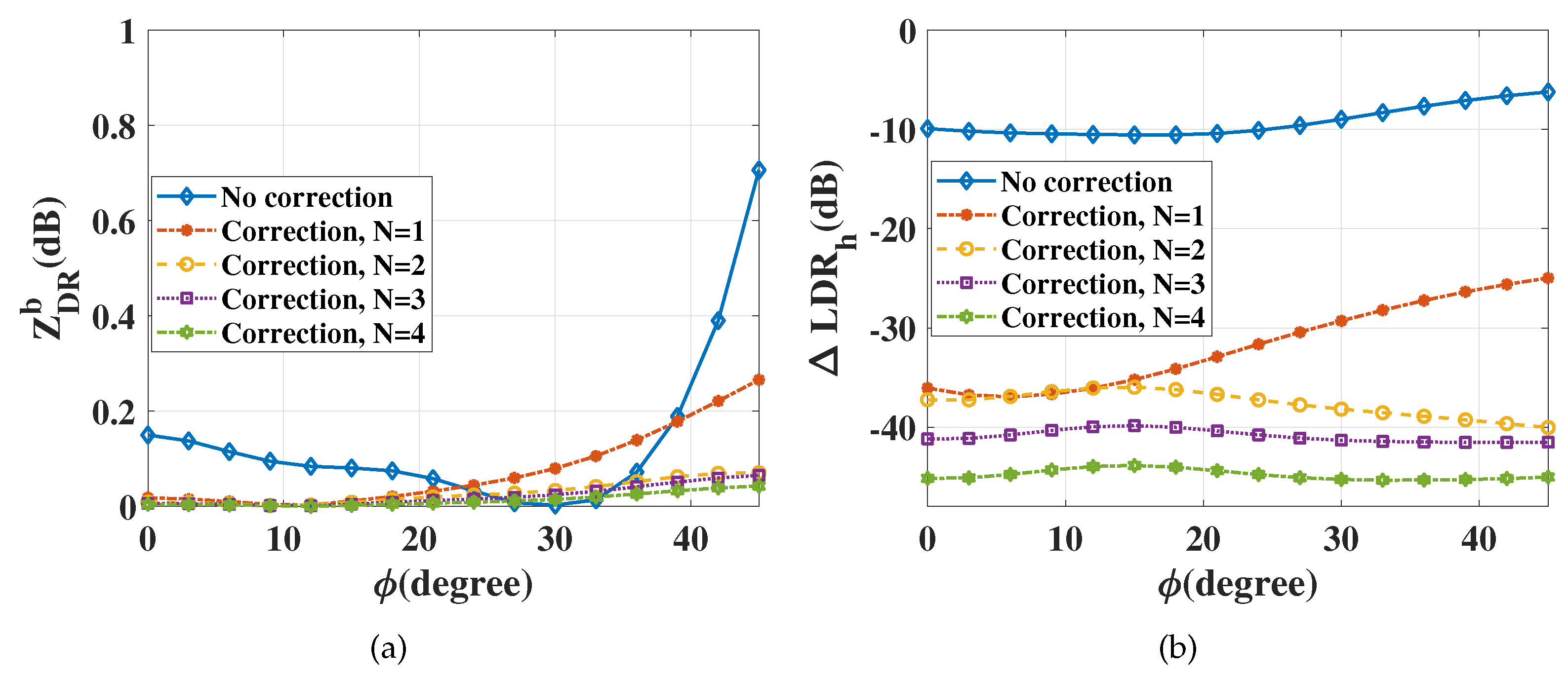
In addition, the influence of the deviation angle on the bias correction is investigated. The polarization characteristics of the wideband array element, especially the non-orthogonal state of the dual-polarized antenna, are very complicated. The co-polarization and the cross-polarization vary with the deviation angle. Taking the bandwidth $B=1700$ MHz, for example, the corresponding results are shown in Figure 9. Without any correction, the $\Delta Z_{DR}$ is very sensitive to deviation angle (fluctuating from 0 dB to 0.7 dB), and the $\Delta LD{R}_h$ keeps large values (around $-10$°). With IFD correction, the $\Delta Z_{DR}$ and $\Delta LD{R}_h$ decrease significantly. Additionally, the correction biases decrease with the increase of N. The correction using the matrix corresponding to a single frequency point cannot meet the accuracy requirement. The $\Delta Z_{DR}$ is greater than $0.2$ dB at several angles and $\Delta LD{R}_h$ reaches $-24.97$ dB. The corrected $\Delta Z_{DR}$ is less than $0.1$ dB over the whole bandwidth if $N\ge 2$, and the $\Delta LD{R}_h$ is below $-40$ dB when $N=3$. Thus, $N=3$ should be considered for this case.

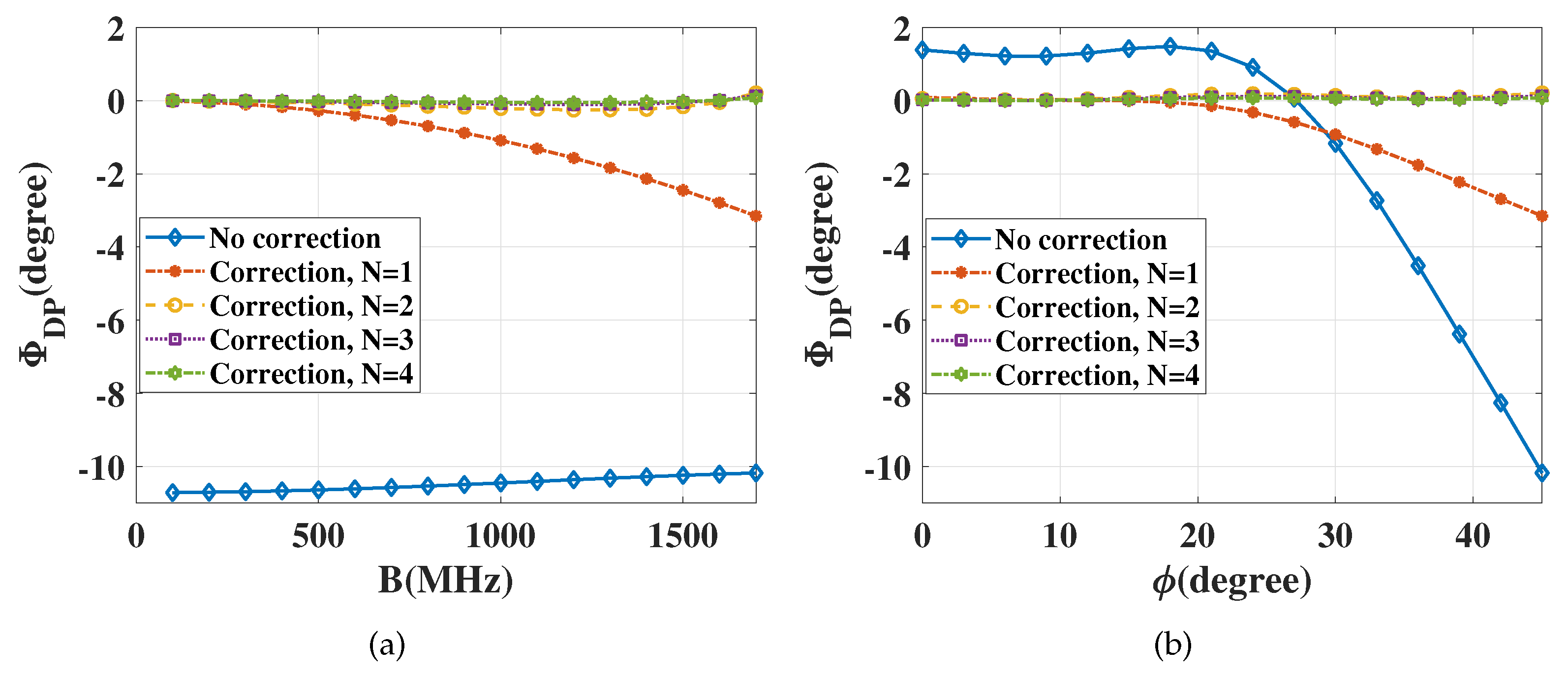
$\Delta Z_{DR}$ and $\Delta LD{R}_h$ are designated as the constraints of bias correction. The simulations present the $\Delta Z_{DR}$ and $\Delta LD{R}_h$, which denote the relationship of the amplitudes between co-polarization and cross-polarization components. To test the validity of the proposed algorithm, the phase of the corrected PSM is investigated. This paper focuses on the differential phase between the two elements of diagonal terms, and it can be corrected similarly, as displayed in Figure 10. The ${\Phi }_{\mathrm{DP}}$ after bias correcting is less than ${3.15}^{\circ }$ under different bandwidths and deviation angles. The bias will be so small that it can be ignored when the corrections are conducted within multiple frequency subbands.

4.3. Discussion

Numerical results and comparisons show that the greater the number of divided subbands is, the smaller the corrected bias will be. However, the computational complexity grows with the increase of the number of divided subbands. The simulations are carried out using MATLAB 2017b (MathWorks, Natick, United States) on a laptop with Intel Core CPU i7-8550U (Intel, Santa Clara, United States) at $1.99$ GHz and 8 GB RAM. The computation time is $5.62$ minutes, $8.02$ minutes, $9.56$ minutes and $10.86$ minutes for $N=1,2,3$ and 4, respectively. According to the given constrained polarization variables, three non-uniform frequency points are enough to make a bias correction. In addition, the time consumed for $N=3$ is 13.6% lower than that for $N=4$. Therefore, we divide the frequency band to three subbands and select three correction matrices corresponding to three frequency points.

In this case, the number of frequency points seems to be small. The reasons may be as follows. On one hand, some idealizations in bias modeling are made, such as the nonlinearity of power amplifier, the amplitude and phase imbalance of H and V channels. On the other hand, the parameters, such as electric field, gain and impedance matching are the function of frequency. These factors contribute to the frequency response of the antenna system which affects the bias correction of the polarization measurement, thereby determining the number of divided subbands. Therefore, N depends on the antenna system parameters. The frequency response of the designed wideband antenna is relatively smooth, as shown in Figure 5b,c. Furthermore, the antenna effective length of an ultrawideband antenna is presented in the frequency-domain in [27], whose amplitude is flat and the phase is linear approximately. Hence, the bias correction operation by several frequency points is enough in the ideal situation.

5. Conclusions

This paper presents a key consideration for the measured PSM bias that arises from the frequency response of the antenna system with wide bandwidth. We propose an IFD method to correct the polarization measurement bias. The measured PSM can be corrected by iteratively multiplying the correction matrices in each subband. The simulation results show that the iterative non-uniform selection of frequency point in each subband is more effective than uniform selection on obtaining the corresponding correction matrix. When the frequency band is divided into three or more parts, it can meet the measurement requirement when the deviation angle varies from $0^{\circ }$ to ${45}^{\circ }$ and bandwidth from 100 MHz to 1700 MHz. That is, $\Delta Z_{DR}$ is less than $0.1$ dB; $\Delta LD{R}_h$ is less than $-40\mathrm{dB}$. The ramification of this paper is that the frequency band division is an effective way to improve the polarization measurement accuracy, especially in the context of wideband antenna system in WPPAR.

An isolated phased array element is analyzed in this paper, without involving the mutual coupling. Future research would investigate the whole array with multiple elements, and the mutual coupling between the elements is necessary to be considered for correcting the bias of polarization measurement.