Fault Detection of a Flow Control Valve Using Vibration Analysis and Support Vector Machine

Abstract

A control valve plays a very significant role in the stable and efficient working of a control loop for any process. In a fluid flow process, the probability of failure of a control valve may increase for many reasons pertaining to a flow process such as high pressures at the inlet, different properties of the liquid flowing through the pipe, mechanical issue related to a control valve, ageing, etc. A method to detect faults in the valve can lead to better stability of the control loop. In the proposed work, a technique is developed to determine the fault in a pneumatic control valve by analyzing the vibration data at the outlet of the valve. The fault diagnosis of the valve is carried out by analyzing the change in vibration of the pipe due to the change in flow pattern induced by the control valve. The faults being considered are inflow and insufficient supply pressure faults. Vibration data obtained is processed using a signal processing technique like amplification, Fourier transform, etc. The support vector machine (SVM) algorithm is used to classify the vibration data into two classes, one normal and the other faulty. The designed algorithm is trained to identify faults and subjected to test with a practical setup; test results show an accuracy of 97%.

1. Introduction

Industrial plants consist of several flow processes to produce by-products. A typical flow process consists of a control valve, which is used to vary the flow rate of flow in the pipe based on the control input. Various types of control valve are available in the market, and these valves are chosen based on the applications depending on the size of the pipe, range of flow rate to be controlled, control input (voltage or current), type of fluid passing through the pipe, and principle of working (electromagnetic, hydraulic, pneumatic, etc.). A pneumatic control valve is one of the widely used control valves [1], and consists of a stem, whose position is varied to increase or decrease the opening in the pipe thereby varying the flow rate of fluid flowing through the pipe [2]. The pressure exerted on the diaphragm connected to the stem results in the movement of the stem. The pressure change is induced by varying the input current applied to the current to the pressure converter, which is the control signal from the controller whose variation is based on the sensor feedback and user input. It can be understood that a pneumatic control valve plays a vital role in the performance of any control loop. Deviation or malfunction of this would lead to a deviation in performance of the control loop and would lead to major problems in the by-product of the industry and hence losses. The causes for a control valve failure in a steam turbine are evaluated in [3]. The effect of improper function of control valves in offshore oil and gas sectors is discussed in the report by the Health and Safety Executive [4]. To understand the present scenarios of control valves in process industries and its effect of faults on the process, a detailed survey was carried out. Reference [5] discusses the effects of valve-induced faults on the performance of industrial loops. The effect of dynamic constraints of a valve such as acceleration and jerks on the system performance is reported in [6]. The cause and effect of stiction fault of a pneumatic valve on the system performance are discussed in [7]. The performance of a steam turbine is analyzed for variation in control valve and actuation system characteristics in [8].

Fault detection and diagnosis of valves are being carried out in many ways. Few of these are reported here; a method for detection of faults in valves in a high-pressure leaching process is discussed in [9]. Valve fault detection for a single stage-reciprocating compressor is discussed in [10]. Detection of a stiction valve fault is discussed in [11], using the pattern recognition technique. A sensor-less, control valve fault-detection method using an observer is discussed in [12]. In [13], fault detection and isolation in a pneumatic control valve used in a flow process are performed using residual evaluation of wavelet transform signal derived from process parameters. Fault diagnosis in actuators is simulated on the Development and Application Methods for Actuator Diagnosis in Industrial Control System (DAMADICS) workbench using fuzzy logic algorithms. Valve clogging, an electro-pneumatic transducer fault, a positioner spring fault and a flow rate sensor fault are reported in [14]. The DAMADICS model is used to generate faults like apositioner supply pressure drop, a partly opened bypass valve and a flow-sensor fault in [15], and an eccentricity data analysis algorithm is used for fault detection. A non-contact process for pneumatic control valve fault detection using a camera and image processing is discussed in [16]. A model predictive controller is designed to stabilize the flow process dynamics even with a stiction fault in [17]. An image of subsystems is processed to detect the faults in [18]. In [19], faults in the pneumatic valve are detected and diagnosed using neuro-fuzzy methods. Reference [20] reported a signature analysis technique based on the hysteresis property of an actuator for fault isolation in pneumatic actuators used for aviation applications. Several pneumatic faults and their fault detection techniques are reviewed in [21]. Both model-driven and data-driven techniques are discussed. This shows the fault diagnosis of valves plays a vital role in any process. Although there are many fault identification algorithms reported in the literature, non-contact type fault identification techniques are widely used and are preferred, because they do not influence the process functionality and due to their ease of installation.

Vibration analysis for fault detection is becoming more prominent in most applications. A deep statistical feature learning method for fault diagnosis of rotating machinery using vibration measurement is considered in [22]. A misfire and valve-clearance faults associated with a combustion engine are detected using vibration analysis in [23]. A method of fault diagnosis for a check valve in a slurry pipeline using vibration signals is formulated in [24]. The time-domain signals of the actuator are analyzed for dimensionality characteristics for fault detection, which is reported in [25]. From the research in this field, it becomes clear that vibration analysis is a cost-effective and non-invasive way to determine faults and monitor a system.

Classification algorithms are becoming a common method for automating a fault detection problem. A fault classification method in an industrial process using support vector machine (SVM)-tree and SVM-forest algorithms is investigated in [26]. A compressor valve fault-detection and monitoring method using an SVM classifier on acoustic emission singles are considered in [27]. For automating a fault detection process, a classification algorithm comes as a handy tool.

It can be seen from the reported works above that a fault can be detected using vibration data and can be automated using a classifier algorithm. Therefore, by combining the techniques, we can achieve an accurate, cost-effective, and non-invasive fault-detection method for a pneumatic control valve. In this paper, a technique is proposed to detect the fault in a pneumatic control valve using an accelerometer to acquire the vibration data. The novelty of this process is that the methods generally used for vibration data analysis are being used to detect control valve faults. By placing the accelerometer on the wall of the pipe, the flow rate can be estimated as described in [28]. It can be inferred that the fault in the control valve will lead to a change in flow rate, which can be detected using vibration data from an accelerometer. Frequency domain data are used as the feature space for classification. The power spectrum density (PSD) of the time domain vibration data is the aspect considered in the frequency domain as the variation in the data was most noticeable in this method as compared to fast Fourier transform (FFT) data. These PSD values are computed for both normal and faulty systems, which in turn are combined to form the training data set. A support vector machine is used to classify between the normal and faulty data from the training set.

Since this method involves a non-contact type of measurement and the detection is done using a machine learning algorithm, this gives us a method to update the detection process to include more faults or to enhance the performance later on. To the best of our knowledge this type of sensing in combination with artificial intelligence has not been carried out on a real-time system regarding control valves.

After the introduction in the first section, the experimental setup used to perform the desired work is discussed, followed by a problem statement, problem solution, results and discussion and finally a conclusion.

2. Experimental Setup

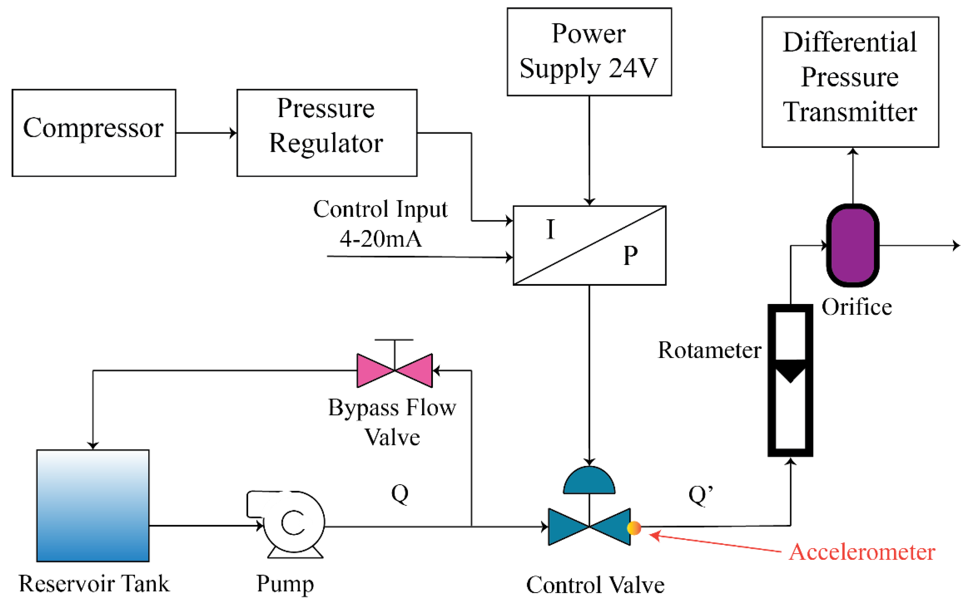
A flow process is considered to demonstrate the proposed algorithm. The process diagram is shown in Figure 1. In the above process, liquid (water) is pumped from the reservoir at a constant rate (Q), a control valve is placed in the path to vary flow rate at the output of the valve (Q’). A bypass path is given at the inlet of the pneumatic control valve for reverse flow. A flow valve is also placed to control the reverse flow. A control signal (4–20 mA) from the controller is given to the pneumatic control valve through an I/P (current to pressure) converter. A rotameter is placed at the outlet of a control valve to display the flow rate (Q’). By varying the control signal, the pressure from the compressor to the I/P converter can be varied and the valve position can be changed which results in a change in flow rate (Q’) at the output of the valve. Furthermore, the flow is directed back to the reservoir, and an orifice flow meter exists to monitor the flow rate via a differential pressure transmitter. 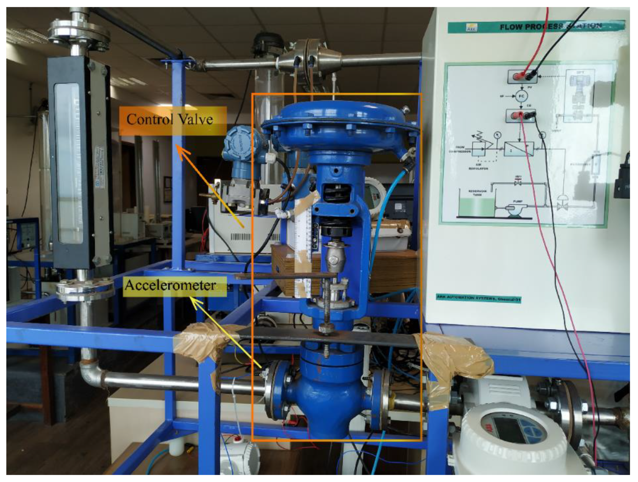Figure 2 shows a picture of the actual process.

Before going into the working of the proposed system a brief introduction to control valves and its faults are discussed here.

2.1. Control Valve

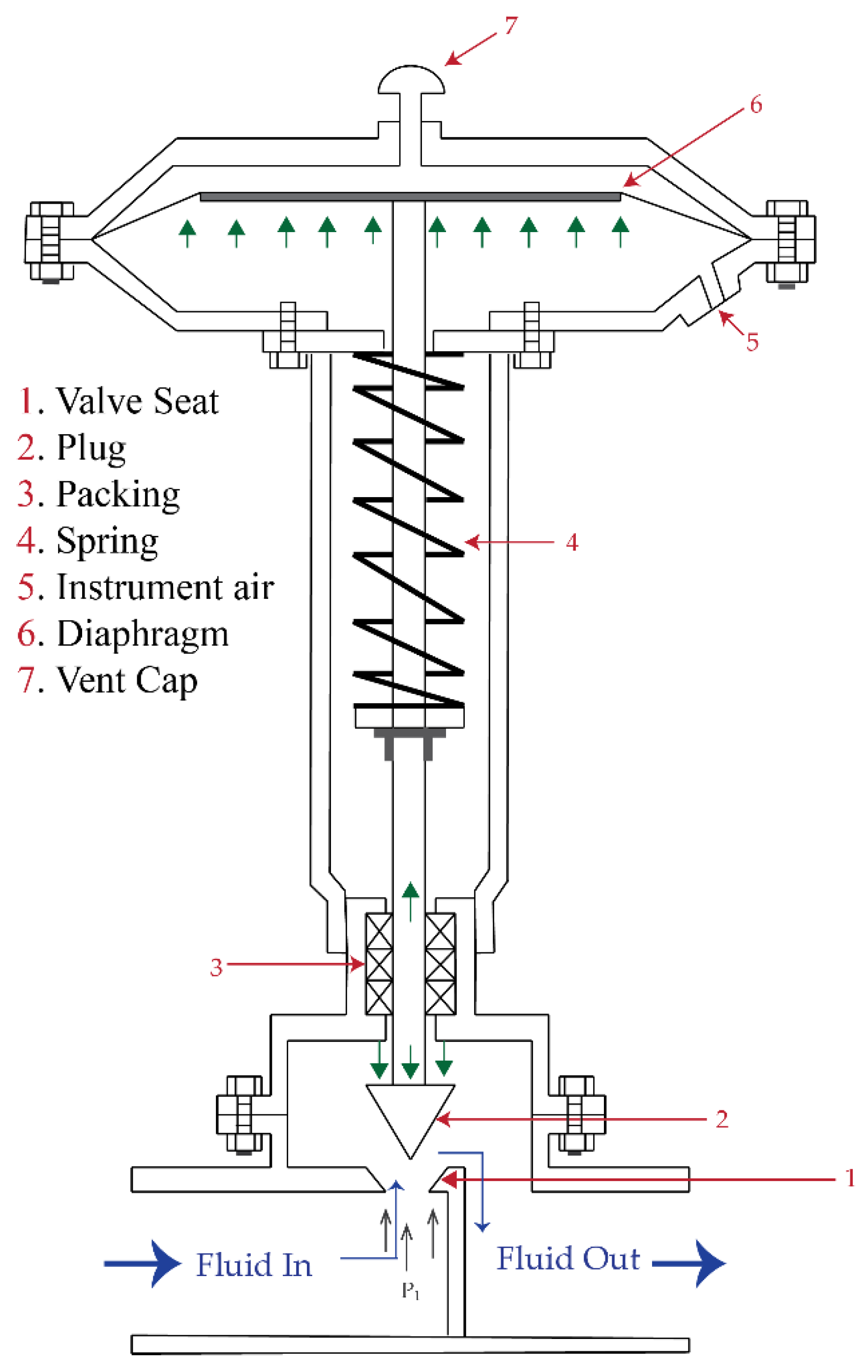
The control valve used in our application is a pneumatic valve which means the actuator used for opening and closing the valve is pneumatic in nature. A cross-section of such a valve is shown in Figure 3 [2]. The purpose of a valve is to hinder the flow of the liquid through a pipe. A valve plug ensures that the proper amount of fluid is transferred to the outlet and based on the design of the plug many flow characteristics can be achieved such as linearity, equal percentage, high flow etc. In the proposed work, an equal percentage valve is considered. The valve plug is attached to a stem, which in turn is attached to a diaphragm as shown above. The diaphragm is placed at the pressure chamber such that when pressure is applied the diaphragm moves up resulting in the upward movement of the stem and valve plug which opens the valve. Since the valve is a normally closed valve, when pressure is reduced the valve closes.

2.2. Control Valve Faults

Pneumatic control valve faults are classified as valve faults, servomotor faults, positioner faults, and general/external faults [2]. Some commonly reported faults are

• Valve clogging—this fault occurs due to dust particles accumulating at the inlet of the valve leading to inaccurate output flow characteristics.
• Positioner supply pressure drop—this fault occurs due to blockage or leak in the supply line and leads to an insufficient supply pressure to the diaphragm, thereby affecting the movement of the stem.
• Fully or partially opened bypass valve—this is due to incorrect inflow because of a malfunction of the flow valve in the bypass path, resulting in erroneous outflow.
• Flow rate sensor fault—can lead to an incorrect measurement of flow rate even though the outflow is correct resulting in the controller making erroneous adjustments.
• Internal leakage (valve tightness)—occurs due to leakage around the valve seat and can lead to a flow of liquid even with a closed valve.
• Stem displacement fault—occurs due to physical misalignment in the stem and can lead to incorrect transmission of movement of the diaphragm to the closing and opening of a valve.

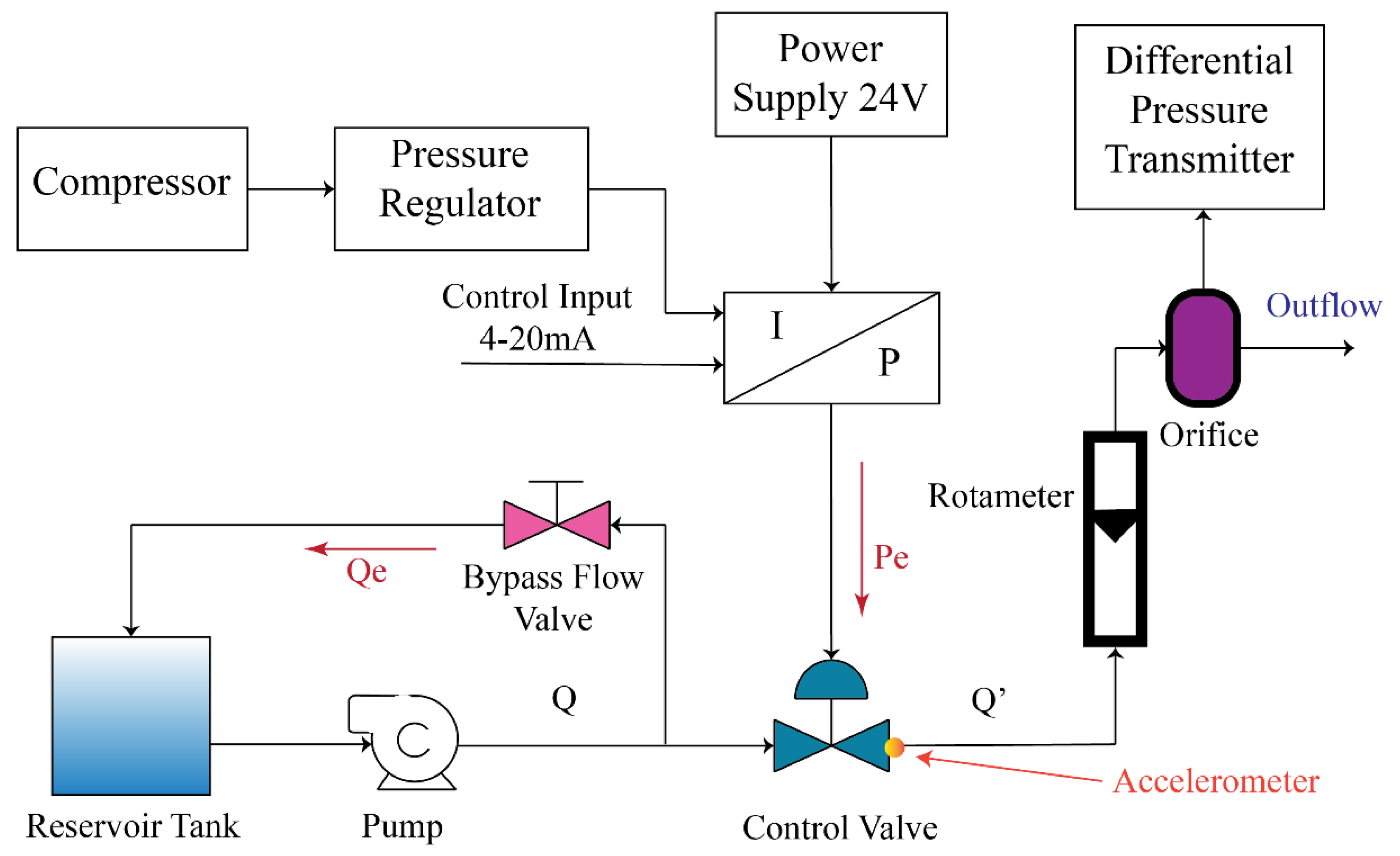
In the proposed work, two types of fault are considered, an inflow fault and an insufficient supply pressure fault, represented in Figure 4 by ‘Qe’ and ‘Pe’, respectively. The former is caused due to the change in the input flow rate of the liquid (here water) and the latter is caused due to lack of pressure to the diaphragm of the control valve itself.

If there is a change in the position of the bypass flow valve in the process, the amount of liquid going back into the reservoir tank varies, which causes the flow rate (Qe) at the inlet of the control valve to either increase or decrease thereby causing the outflow to vary resulting in an error. This error is referred to as the inflow error. The flow rate at the output is controlled by the control valve by varying the stem position, which is excited by the pressure at the diaphragm chamber. Excitation pressure is supplied at a value greater than the control pressure of 3–15 psi. If the excitation pressure (Pe) is kept less than control pressure, the diaphragm will not be able to cause movement to the stem position as expected. The resulting fault is termed the insufficient supply pressure error. The resulting changes in the flow rates due to these induced errors at the output of the control valve are detected by the accelerometer as a change in vibration and are used by the detection algorithm.

Both the inflow fault and insufficient fault cause variation in the outlet flow even with a proper control signal, and this change in outflow will affect the process stability. Hence to avoid this situation it becomes necessary to detect the error so that the controller can be notified of the cause of error at the output and a suitable method can be designed to incorporate the additional information into the controller. A method is proposed to identify both faults automatically.

3. Methodology

To detect the faults mentioned above, a system is proposed that uses non-invasive techniques using vibration analysis. An accelerometer is placed at the outlet to obtain the vibration data needed for the detection. Since it is possible to estimate the flow rate using a vibration sensor as mentioned in [28], it will also be possible to detect a fault in the flow rate.

The placement of the accelerometer is considered first by taking into account that any changes in the control valve operation are directly reflected at the output of the valve. Second, it is seen that the flow becomes uniform after a distance of over “6 times pipe diameter from the valve” which would mean that the lower the effect of vibration the farther the accelerometer is placed. In the proposed work, a distance of two times the diameter of the pipe from the coupling of pipe and valve is maintained. Third, any controller in the process would use the output flow rate as the parameter to be monitored and any changes in this would affect the controller operation, hence it is intuitive to measure the same.

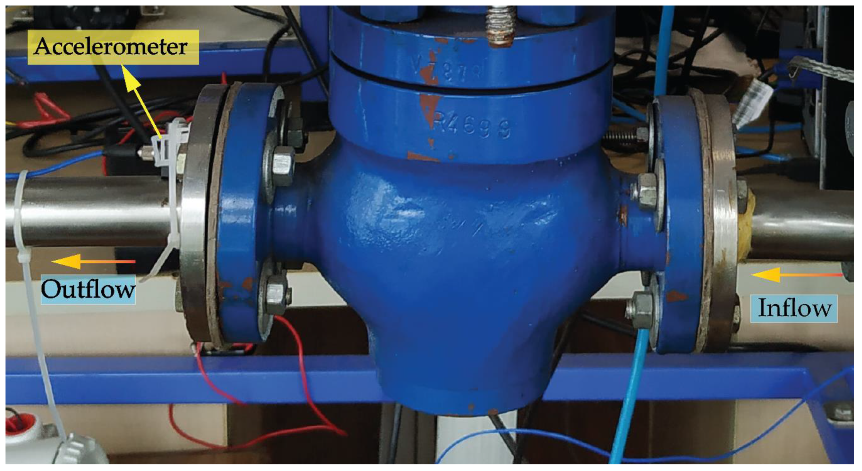
The accelerometer is placed near the output of the control valve, as shown in Figure 5, which gives us the vibration data of the control valve for changes in the flow. Sensor placement is considered based on the point of maximum vibration, as the sensor is coupled to the flange of the valve. The acquisition setup consists of a PCB 352C03 ceramic shear ICP^® accelerometer, which is a single axis vibration sensor with a sensitivity of 10 mV/g and frequency range of 0.5 to 10000 Hz [29].

The NI 9234 Sound and Vibration module, which is designed for the measurement of IEPE (Integrated Electronics Piezo-Electric) sensors, is used for the acquisition and conditioning of the accelerometer data. This module needs either a CompactDAQ or CompactRIO or a Carrier module. Since processing power is not required for the proposed method, a carrier was enough to acquire data.

The accelerometer (PCB 352C03) is a single-axis accelerometer hence only one-dimension data is considered for this process. Although multi-axis accelerometer can also be used, it will lead to large feature set hence longer computation time. In order for the vibration data to be analyzed, data has to be acquired, this is achieved using a NI Sound and Vibration input module (NI 9234) in conjunction with a wireless and ethernet carrier (NI WLS 9163). NI WLS 9163 is a wireless or ethernet interface for an I/O module. Here we have used the Ethernet port for connectivity. Using NIMAX, the acquisition setup has been configured for later use in MATLAB’s data acquisition module. MATLAB’s data acquisition module is used to acquire the data into MATLAB for further processing. The SVM algorithm is implemented using MATLAB built-in classifier libraries. The workflow is shown in Figure 6.

3.1. Vibration Analysis

For the purpose of vibration analysis, all the vibrations can be considered to be combinations of sine waves. This forms the basis for frequency domain analysis of vibration data. Because all the time domain data can be summed up to have sinusoidal waveforms of different frequency, it makes sense to perform further analysis in the frequency domain. For this, a Fourier transform is used, and since our application needs digital inputs, we consider a discrete Fourier transform as given in Equation (1) [30]:

$$\mathrm{S}({\mathrm{f}}_{\mathrm{k}})={{\displaystyle \sum }}_{i=0}^{N-1}s(t_i){\mathrm{e}}^{-\mathrm{j}2\pi {\mathrm{f}}_{\mathrm{k}}{\mathrm{t}}_{\mathrm{i}}}({\mathrm{t}}_{\mathrm{i}+1}-{\mathrm{t}}_{\mathrm{i}})\hspace{1em}\hspace{1em}\mathrm{k}=0,1,...,\mathrm{N}-1,$$

(1)

where S(f_k) is the frequency domain data for a given data s(t_i) in the time domain. N is the number of data points after sampling.

Power spectrum density is the best option if the vibration data is random, with no prior knowledge of the mode of vibration [31]. Power spectral density gives the energy for the whole period considered, distributed about the normalised frequency.

Due to the sampling of the data involved to get the data into MATLAB, there can be a discontinuity in the acquired image, which causes power leakage in the frequency domain. To reduce this effect, we need a window function for the FFT or PSD computation. In our case, the best-suited window was found to be a Hanning window of length 2048. The Hanning window equation is given as in Equation (2) [32]:

$$w(n)=0.5(1-\cos (2\pi \frac{n}{N})),0\le n\le N,$$

(2)

where w(n) is the window function, N is equal to one less than window length.

Most applications using vibration analysis discussed in the introduction use the vibration measurement of the instrument itself, but here the accelerometer does not measure the vibration associated with control valve, rather the vibration due to the flow of liquid in the pipe at the outlet of the control valve. Placement of the accelerometer directly on the control valve will affect the vibration data obtained, whereas in the proposed work the vibration data is more discernible towards the estimation of the fault.

3.2. Support Vector Machine (SVM)

The support vector machine is a classification method where the classes are divided by a decision boundary. The type of boundary depends on the number of features, in a two-feature one-class SVM classifier, the decision boundary will be a line (both linear or a higher-order polynomial function). Similarly, the decision boundary will be a line in a hyperplane for more features. In this work, since the vibration data obtained is random and hard to quantify using models or equations, a more generalised classification algorithm is needed [33]. A simple logistic or linear regression does not have the robustness associated with the SVM needed for the proposed application. As the requirement was a binary classification, there was no need for a neural network classification.

The raw vibration data acquired from the NI module into MATLAB is hard to distinguish for the SVM classifier. Hence, the time domain data is converted to the frequency domain for a better understanding, as explained earlier. FFT did not produce many details compared to PSD, as shown in Figure 7. Hence, power spectrum density will be used as the frequency domain data for the SVM classifier.

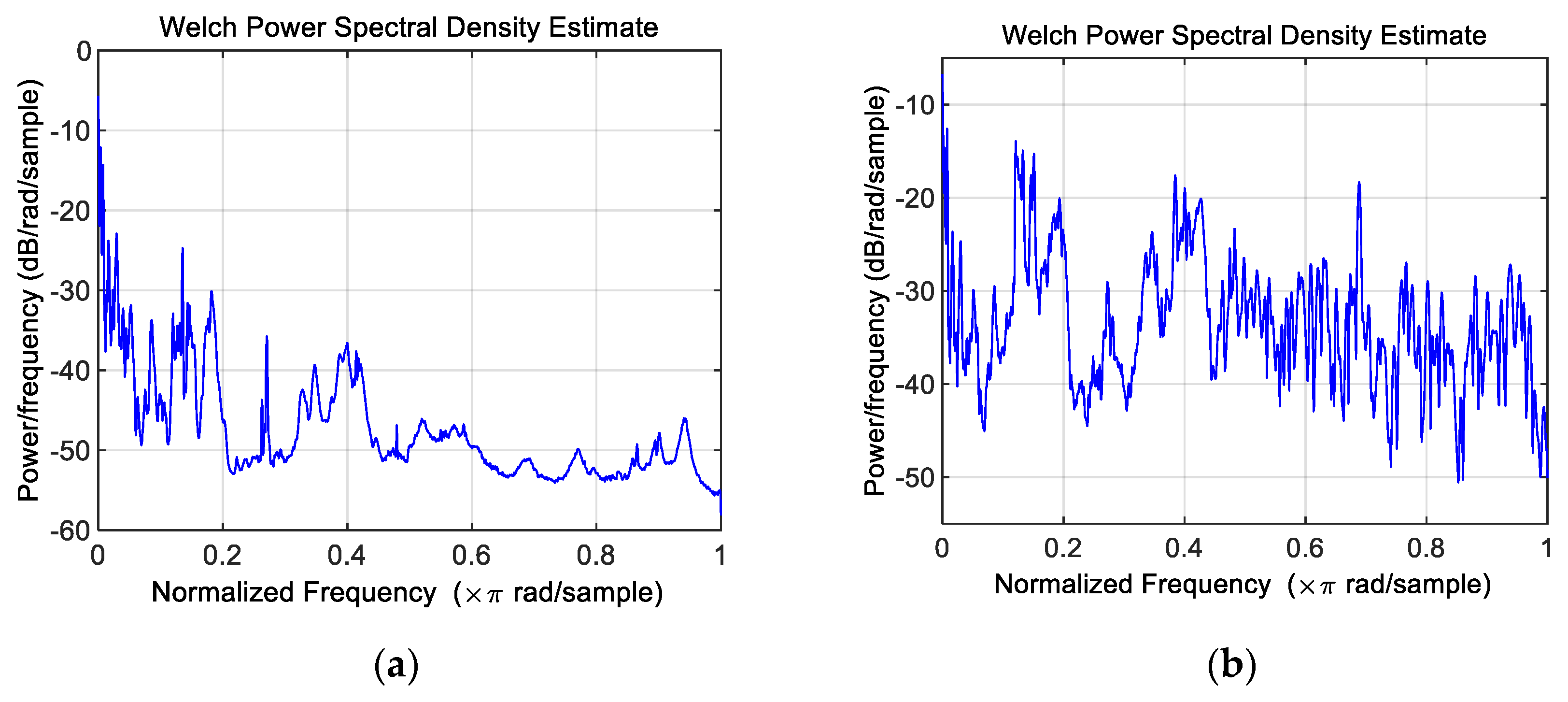
By adjusting the window function used for frequency domain analysis, a better frequency division of raw data is obtained. By comparing the normal PSD values with faulty PSD value, the difference is noticeable as shown in Figure 8.

As seen from Figure 8, considering the data as a pattern instead of single data for classification will be intuitive, since the difference is most apparent when considered as a whole pattern.

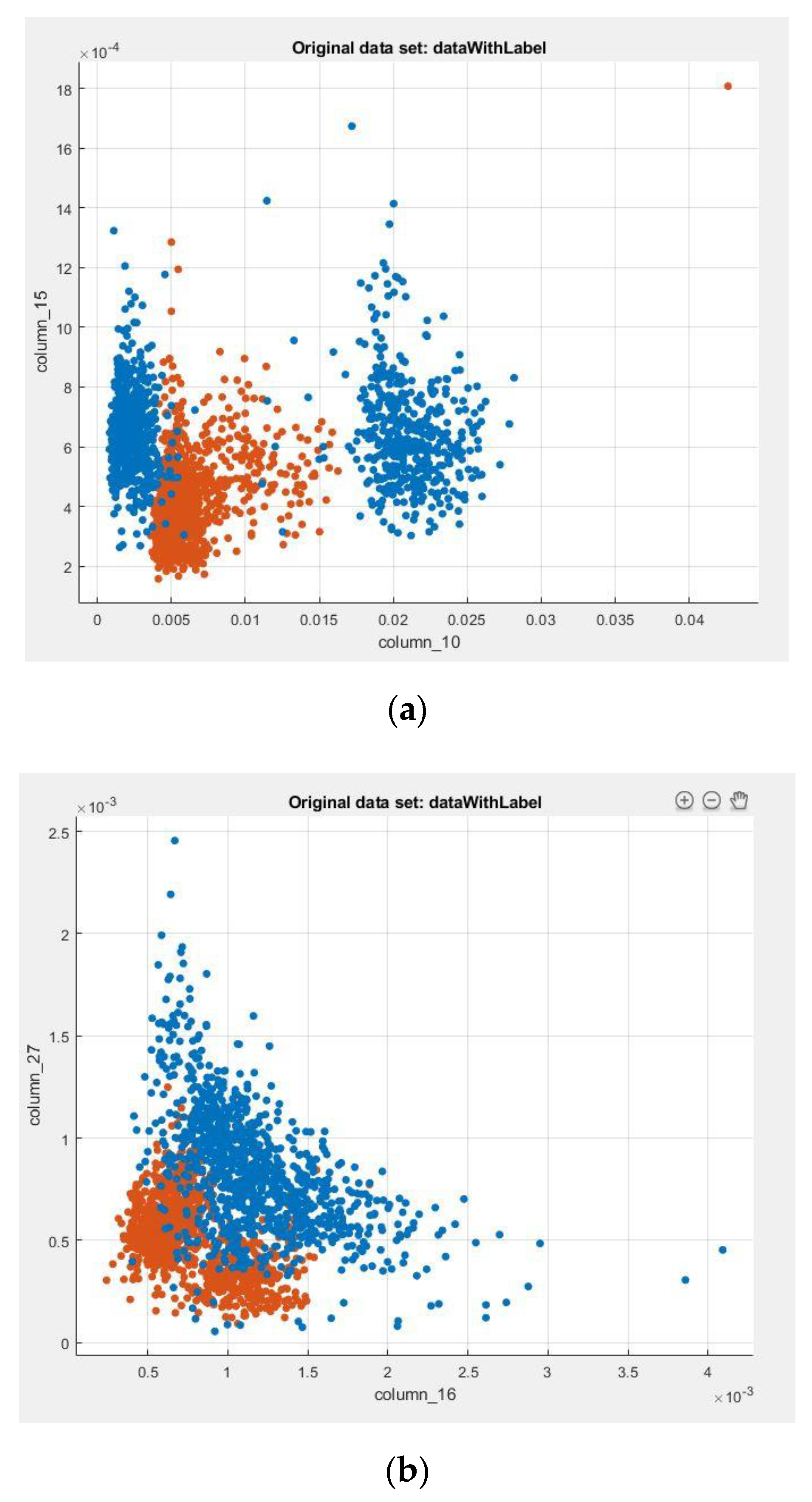
Once the data is processed as required, it can be used for the classification by selecting the features from the computed PSD data. Here, the features are chosen such that the pattern of variation of vibration data from one sampling time makes up the entire feature space. This will be similar to a pattern classification in an image-processing application. In choosing this method, only the vibration associated with faults consisting of a different pattern to that of normal vibration data will be classified as faulty. Since the features will be around 2000, data sets for training were chosen to be around 4000 to get a more accurate model. Figure 9 shows scatter plots of some columns of the feature set. The blue points indicate normal data and red points indicate faulty data. It can be seen from these plots that the faulty data is distinguishable. By combining many such features, a training model is obtained.

The model used for training the SVM classifier is a Gaussian kernel or radial basis function, which is given by Equation (3) [34]:

G(x₁, x₂) = exp(−‖x₁ − x₂‖²),

(3)

These features are then fed to the SVM classifier function along with its label vector for training the SVM model. The best results were obtained using the Gaussian kernel and cross-validation of five folds.

4. Results and Analysis

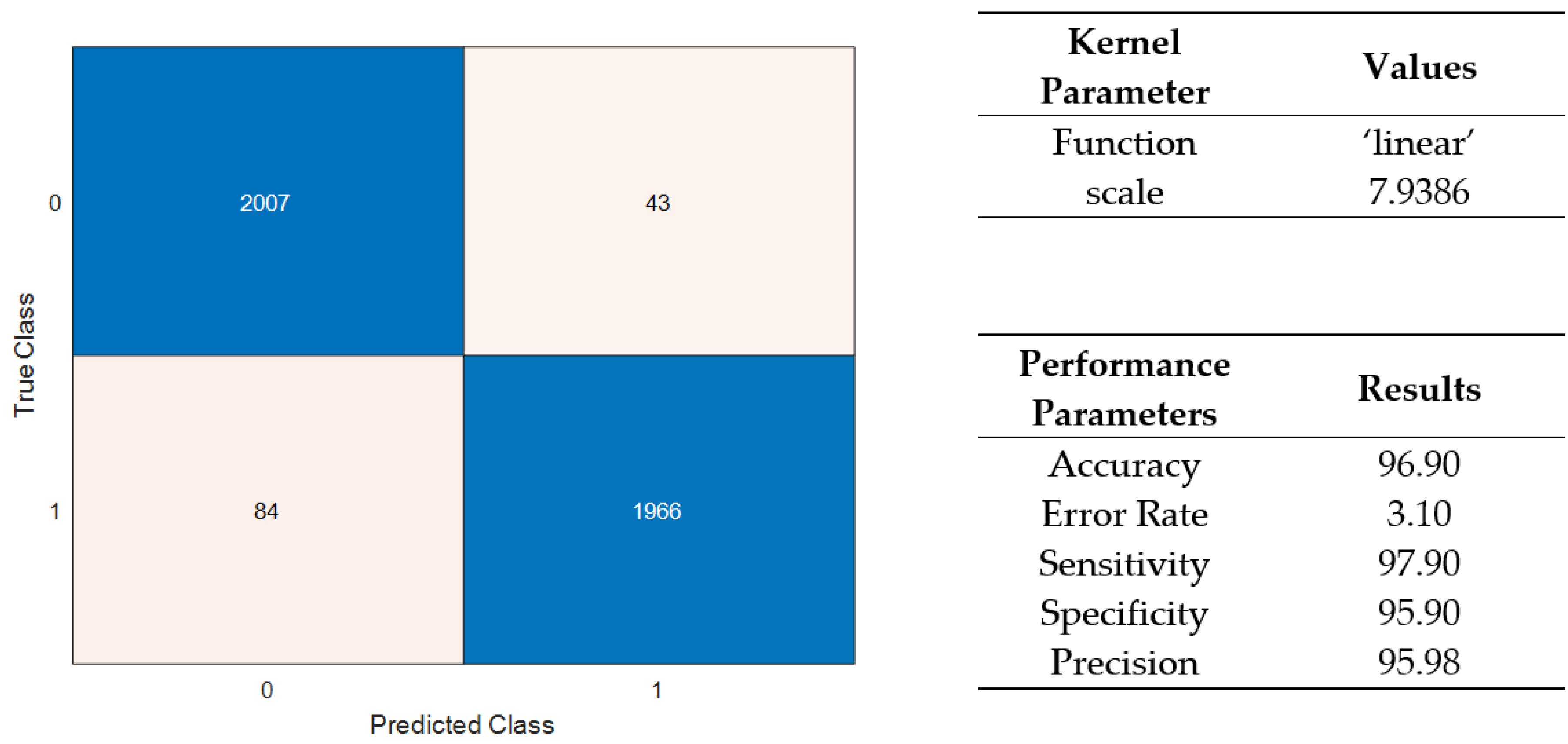
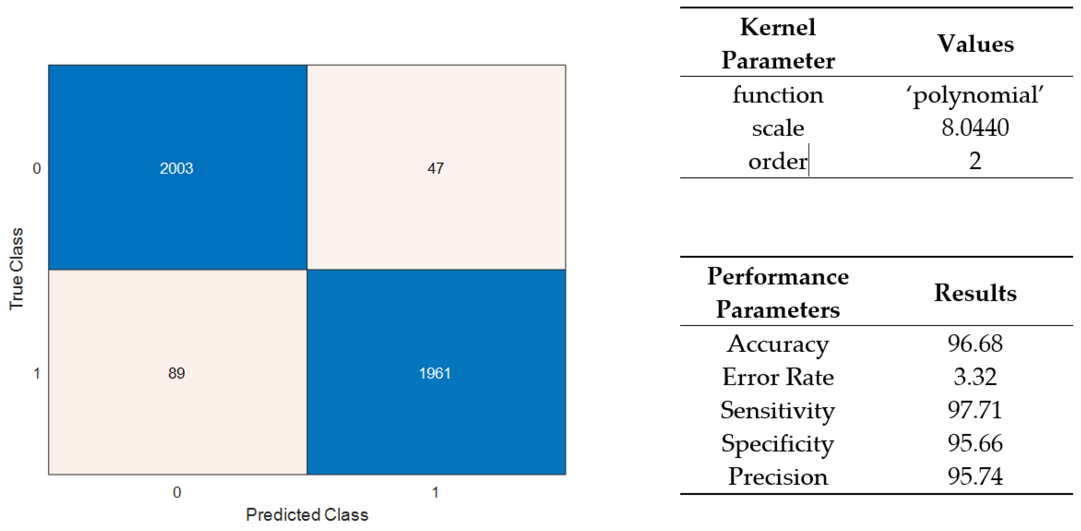
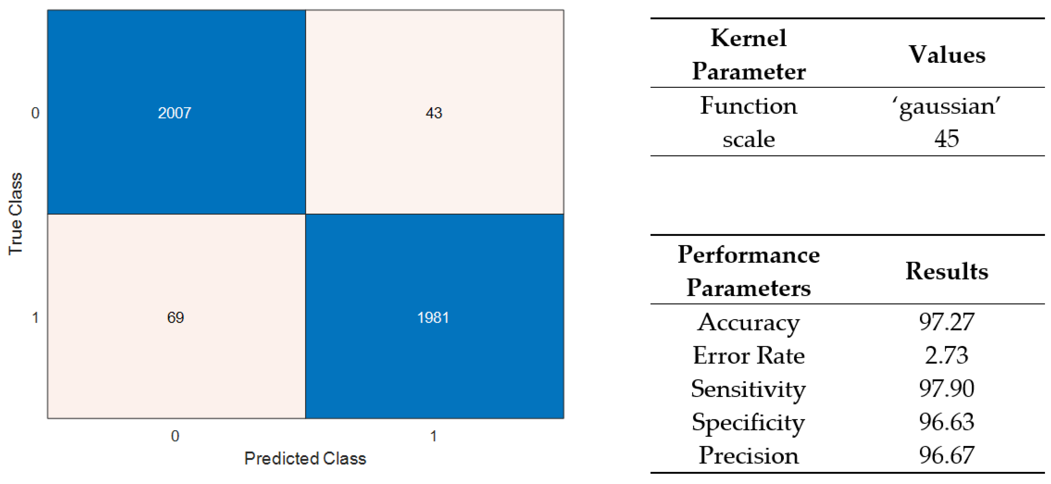
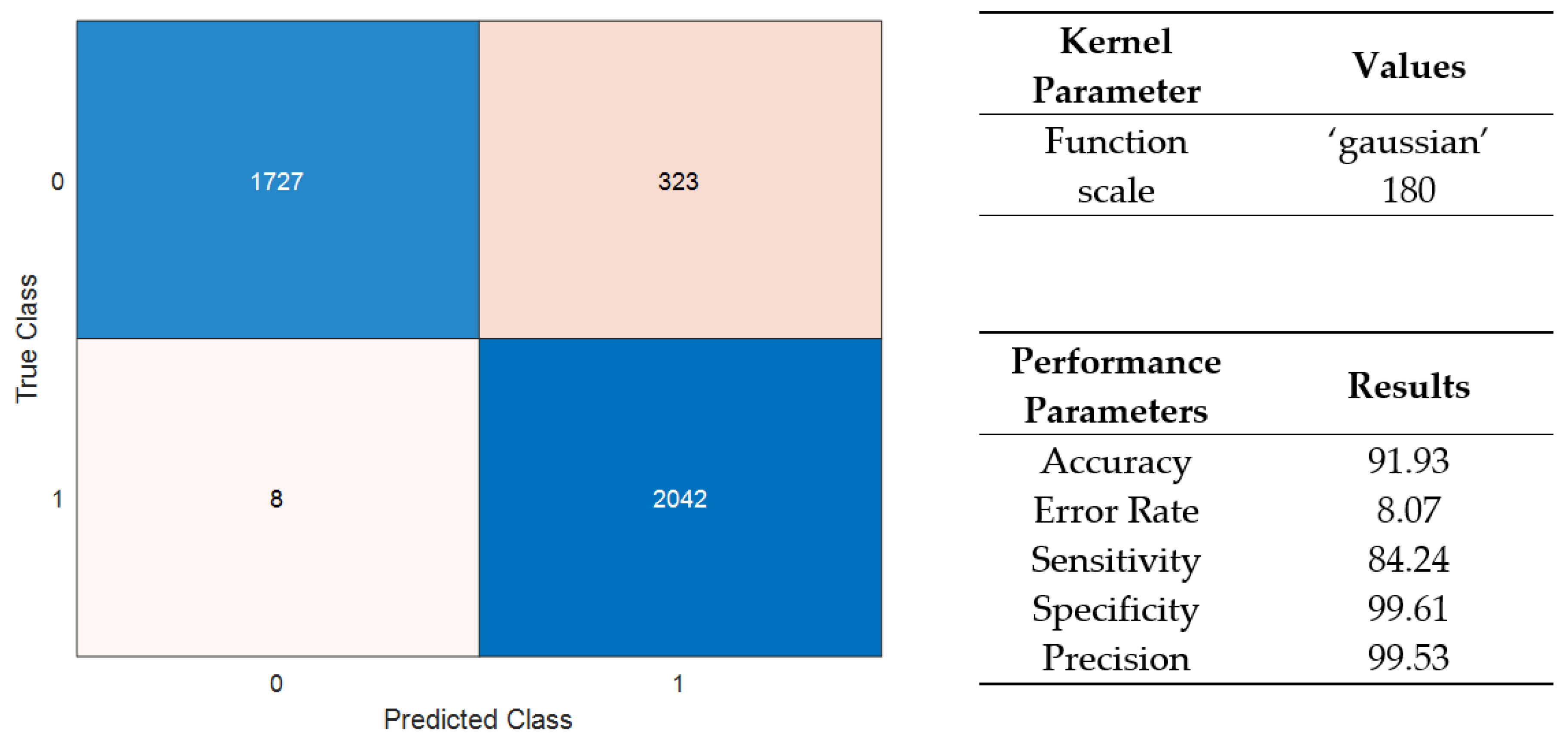
Implementing the SVM in MATLAB, a trained model is obtained with the feature set, as mentioned earlier. The label vector consists of ones for normal data and zeroes for faulty data. By modifying the parameters such as the type of kernel and cross-validation folds, various results were obtained for comparison. The best possible model with the most accuracy was selected for further prediction. A test data set was used for prediction, which gives a prediction vector consisting of predicted class labels associated with the test data. By comparing the predicted class labels with the class labels of test data, a confusion matrix can be created as shown in Figure 10. After computing the confusion matrix of the obtained results, the accuracy was found to be 97%. This implies that when a data set is classified as either faulty or not faulty, then 97% of the time it is correctly classified.

The fault diagnosis technique designed is tested by subjecting it to various flow conditions. Two faults, namely input flow and supply pressure, are manually induced. The control valve is designed to operate between 3 and 15 psi, which is controlled by the control input current of 4–20 mA. This conversion is done by an I to P converter. This I to P converter needs a supply pressure of 18 psi to function as an excitation source for the control valve. If the pressure is less than the actual pressure of 18 psi, it is said to be faulty. This fault might happen due to leakage or breakage in the connecting tube.

Similarly, it is desired to have a constant inflow of liquid to the control valve. In the proposed experiment, 2000 lph is the inflow that is maintained by the pump. This inflow can be regulated by varying the bypass valve position to induce the inflow error. If the bypass valve is fully closed, the inflow rate would be at its maximum, which is related to the pump rating. When the bypass valve is fully open, the inflow rate at the valve would almost reduce to zero. To validate this, a test is conducted by changing the control valve position with a varying control current signal; in normal working conditions the outflow should change according to the control signal. However, by changing the bypass valve position, the outflow rate differs from the normal operation even though the control signal remains the same as before.

The experiment is tabulated as shown in

Table 1. Test results of fault-detection technique.

Control Input (mA)	Supply Pressure (psi)	Inflow Rate (lph)	Measured Outflow Rate (lph)	Condition Identified
5.2	18	2000	80	OK
14	18	2000	610	OK
10	0	2000	0	Fault
18.5	2	2000	0	Fault
18.5	18	2000	900	OK
12	18	300	240	Fault
4.2	18	100	0	Fault
17	10	2000	300	Fault
12	3	200	100	Fault

. The first column of Table 1 shows the control signal in terms of mA obtained from the controller. The second column represents the supply pressure given to the I to P converter. If the supply pressure is less than a rated control pressure of 3 to 15 psi, the operation of the control valve will be affected. The third column gives the inflow rate at the valve. In the normal operation, the inflow is the same as the flow rate obtained from the pump. Desired outflow is expected to be between 0 and 1000 lph, where 0 corresponds to 4 mA of the control signal and 1000 lph corresponds to 20 mA of the control signal. The measured outflow is given in the fourth column. The last column of the table gives information about the condition of the valve.

The proposed technique is tested by varying the control signal from 4 to 20 mA. On varying the control signal, we can see that outflow would vary proportionally as shown in serial numbers 1, 2, and 5 in Table 1. In other cases, a fault is induced by varying the supply pressure and inflow rate. It can be observed that this leads to abnormal behaviour, producing outflow that is not proportional to the control signal. Results identified by the proposed classifier are shown in the last column. Only a few test results are included here.

Similar tests were repeated with different operating conditions by varying the control signal with and without induced faults in the system. Out of the 224 fault-induced test cases, the system could detect the fault in 217 cases. From the above results, it is clear that the proposed fault detection technique can be used on a real-time application.

Once the system is trained with the offline data set, it can be subjected to a test in real time in an online mode. For this the trained set should be dumped on the real-time target device like a NI cRIO (CompactRIO) and the signal from the vibration sensor and the control signal directly captured by the NI cRIO using analog channels.

Performance

Performance matrices can be calculated from the confusion matrix as described below [35]:

• Accuracy = (TP1 + TP0)/TS. This defines how well the classifier can distinguish between classes.
• Error Rate = (FP1+ FP0)/TS. Similar to accuracy but considered in terms of the wrong prediction.
• Sensitivity =TP0/ T0. This tells us how well the fault vibration data can be detected by the training model.
• Specificity =TP1/T1. This quantifies how well a normal vibration data can be detected by the training model
• Precision =TP0/P0. This parameter gives us an estimate of how often the fault predicted is actually faulty.

Here, TP1 is the number of samples truly predicted as class 1; TP0 is the number of samples truly predicted as class 0; TS is total test samples used for prediction (in our case 4100); FP1 is the number of samples falsely predicted as class 1; FP0 is the number of samples falsely predicted as class 0; T0 is the total number of samples that belong to class 0; T1 is the total number of samples that belong to class 1; P0 is the total number of samples predicted as 0; Class 0 is the class associated with faulty vibration data and Class 1 with normal vibration data.

From Figure 11 and Figure 12, it can be inferred that, even though the accuracy is not the best, the sensitivity is high, leading to better fault detection. From Figure 13 it can be inferred that both accuracy and sensitivity are high, leading to better detection of fault compared to all other models. Although it can be seen from Figure 14 that this model predicts normal vibration data better than any other model, since specificity is very high the faulty data will be considered as normal data more often. Therefore, if this model predicts that the data is faulty then the chances of it being right are very high since precision is 99.53%. From all the above results, it can be seen that some models have advantages over the other and only the accuracy cannot be a determining factor. In addition, by combining two or three models’ data, better prediction can be achieved.

A comparison of performance of some of the existing methods for detection of faults in control valve is shown in

Table 2. Comparison of performance with existing work.

Paper	Performance
[8]	95% accurate under simulation
[9]	93.2% accurate for wear fault detection under simulation
[11]	78% accurate under simulation
[13]	95% accurate under simulation
[14]	89% accurate
[36]	95% prediction accuracy under simulation

.

5. Discussion

Identification of faults in a pneumatic control valve is very essential as the flow process is a quick process, and many physical parameters are controlled directly or indirectly using the flow data, like pressure, temperature, etc. Pneumatic control valves are also used in pharmaceutical and dye-manufacturing companies for manufacturing products by mixing different parameters. Reported work considers the use of a vibration sensor for fault identification in the control valve. Vibration sensors are considered because of their non-invasive characteristics. Fault identification techniques are designed using SVM classifiers. The results obtained from the tests conducted show that it is possible to detect a fault in the control valve by using vibration data as the predictor with good accuracy. In the reported work, only two of the errors normally occurring in a control valve operation like inflow fault and insufficient supply pressure faults were considered. The reported method could detect faults with an accuracy of 97%. As compared to the existing works, as seen in Table 2, where most of the papers spoke about simulation results, the proposed worked showed better results. The model can be further improved to include other errors such as actuator vent blockage, diaphragm leakage.