Article

Efficient Emergency Load Shedding to Mitigate Fault-Induced Delayed Voltage Recovery Using Cloud–Edge Collaborative Learning and Guided Evolutionary Strategy

1
Hainan Power Grid Co., Ltd., Haikou 570203, China
2
Global Institute of Future Technology, Shanghai Jiao Tong University, Shanghai 200240, China
*
Author to whom correspondence should be addressed.
Electronics 2026, 15(7), 1377; https://doi.org/10.3390/electronics15071377
Submission received: 10 January 2026 / Revised: 5 March 2026 / Accepted: 10 March 2026 / Published: 26 March 2026
(This article belongs to the Section Power Electronics)

Abstract

Fault-induced delayed voltage recovery (FIDVR) poses a serious threat to modern power grid operation, where stalled induction motors following a fault can sustain dangerously low bus voltages and potentially trigger cascading failures. While deep reinforcement learning (DRL) has shown promise for emergency load shedding control, existing centralized DRL approaches require extensive communication infrastructure and large neural network models that are computationally prohibitive to train at scale. Fully decentralized approaches, on the other hand, lack inter-agent information sharing and coordination, often resulting in inadequate voltage recovery across area boundaries. To address these limitations, we propose a Cloud–Edge Collaborative DRL framework that combines lightweight, area-specific edge agents for local load shedding control with a supervisory cloud agent that coordinates their actions globally, achieving scalable training and system-wide voltage recovery simultaneously. Training is further accelerated through a modified Guided Surrogate-gradient-based Evolutionary Random Search (GSERS) algorithm. Validation on the IEEE 300-bus system demonstrates that the proposed framework reduces training time by approximately 90% compared to the fully centralized approach, while achieving comparable voltage recovery performance to the centralized method and approximately 80% better reward performance than the fully decentralized approach, confirming the critical benefit of the cloud-level coordination mechanism.

1. Introduction

Modern power grids face new challenges as an increasing number of inverter-based renewable resources and variable loads are connected to the system. Faults can cause bus voltages to remain depressed for several seconds even after the fault clears, a phenomenon known as fault-induced delayed voltage recovery (FIDVR) [1]. This phenomenon occurs primarily because induction motors stall under low-voltage conditions and absorb large amounts of reactive power during the stall stage, while protection devices require time to trip the stalled motors [2]. FIDVR events threaten grid stability and can trigger cascading failures that propagate across wide areas of the grid [3].
The current industrial approach to mitigating the FIDVR problem is to perform load shedding to trip stalled motors and thereby reduce the excessive reactive power demand of the stalled motor loads [4]. Existing load shedding methods deploy fixed rules based on predetermined voltage thresholds [5], but these rules do not account for coordinated load shedding across different locations and therefore often result in excessive load curtailment. In other words, rule-based approaches tend to shed more load than strictly necessary to ensure safe system operation, and these excessive load shedding actions severely inconvenience electricity customers who experience supply interruptions. Researchers have proposed more sophisticated methodologies to identify appropriate shedding locations and minimize the load shedding amount required to restore system voltage, including security-constrained optimal power flow [6], coordinated inverter control [7], and  model predictive control [8]. These approaches require detailed grid models and intensive computation, making them difficult to apply in real time, given that load shedding decisions must be made within a few seconds of a FIDVR event to prevent the voltage problem from propagating through the system.
To overcome the limitations of model-dependent methods, researchers have turned to data-driven approaches that circumvent the need for accurate grid models. Decision trees [9] and extreme learning machines [10] can learn patterns from measurement data to make load shedding decisions that adapt automatically to different operating conditions. Deep reinforcement learning (DRL) goes further by enabling agents to discover effective load shedding strategies through trial and error [11,12]. A DRL agent is a neural network (referred to as a policy network) that interacts with the grid environment, receives feedback on its actions, and iteratively improves its policy. The DRL paradigm effectively combines principles from adaptive control theory with deep learning frameworks, enabling agents to learn optimal action policies through environmental interaction and cumulative reward maximization over training iterations. Various DRL methods for solving the Markov decision process (MDP) have been proposed, including value function methods [13], policy gradient techniques [14], and hybrid approaches [15]. Over recent years, DRL has been applied to a wide range of power system problems, including battery dispatch in microgrids [16], damping of power oscillations [17], and volt-var optimization in distribution networks [18]. Recent advances have further extended DRL to broader power system operation tasks, including frequency regulation and active power balancing under high renewable penetration [19], as well as robust distributed voltage control in multi-feeder distribution networks [20]. Building on this progress, we develop a scalable DRL framework using cloud–edge computing for emergency load shedding to address the FIDVR problem in large-scale power grids.
Current DRL-based emergency load shedding control strategies typically adopt centralized control architectures, in which a single controller aggregates measurements from buses at different geographic locations and dispatches control commands to multiple load shedding points throughout the network. This setup requires extensive communication links connecting the control center to geographically dispersed sites, and any failure in these links can disable the entire control architecture. Furthermore, training a single neural network policy to handle a large-scale grid is time-consuming, as the network must have a large number of parameters whose space must be explored extensively across the high-dimensional operating conditions of the large-scale power grid to ensure adequate tuning. Conversely, reducing the neural network size shortens training time but significantly degrades control performance. This scalability issue becomes particularly acute in large-scale power grids. As the grid size grows, the dimension of the observation space increases with the number of monitored buses, and the action space expands with the number of controllable loads available for shedding. Moreover, the dynamics of large-scale grids are considerably more complex, necessitating a larger policy network as well as substantially broader coverage of operating conditions and fault scenarios during training. Together, these factors cause the training time of a centralized DRL agent to grow dramatically with system size, making centralized approaches impractical for real-world large-scale power grid applications. This scalability bottleneck is the critical motivation behind the development of the proposed Cloud–Edge Collaborative DRL framework. Decentralized designs avoid these problems by placing independent controllers in each area of the power grid. However, the drawback of decentralized control architectures is that these controllers do not share information with one another and therefore lack coordination. Without full system observability and proper inter-area coordination, the load shedding actions taken independently by decentralized agents may result in sub-optimal load curtailment or inadequate voltage recovery in neighboring areas.
Deep learning and deep reinforcement learning (DRL) have recently attracted significant attention for fault detection, fault diagnosis, and fault-tolerant control in power electronic systems and power grids. For fault detection in power converters, Kiranyaz et al. proposed a real-time fault detection and identification scheme for modular multilevel converters (MMCs) using adaptive one-dimensional CNNs that process raw voltage and current signals directly, achieving high detection accuracy while operating in real time [21]. Han et al. combined short-time wavelet entropy with an improved LSTM network to diagnose faults in MMCs from sampled current data [22]. Ye et al. proposed a wavelet packet and LSTM-based method for simultaneous fault diagnosis and fault-tolerant reconfiguration in five-level nested neutral-point-piloted converters within a unified framework [23]. Fan et al. developed an LSTM-based approach to detect multiple open-circuit faults in MMC systems under various operating conditions [24], and  further extended this to a hybrid perturbation estimation convolution network (PECN) for simultaneous fault detection and location in cascaded H-bridge multilevel converters [25]. More recently, Teimouri et al. proposed a hybrid CNN and reliability-based fault detection and location (HCNN-FD-RFL) method for short-circuit faults in multilevel inverters, achieving fault detection in approximately 45 μs using only a single voltage sensor [26]. Beyond component-level fault diagnosis, DRL has also been applied to fault-tolerant control at the power system level. Igder et al. applied DRL to service restoration in distribution networks [27], while Zhang et al. demonstrated DRL-based intelligent fault-tolerant active power control for wind farms [28]. It is important to note that the DRL framework proposed in the present paper operates on a fundamentally different principle from the fault detection and fault-tolerant control approaches reviewed above. Our DRL agent does not perform fault detection or component-level fault identification; instead, it directly observes the bus voltage trajectory following a disturbance and makes continuous real-time load shedding decisions based solely on the observed voltage conditions, without any explicit fault identification step. This design deliberately bypasses the fault detection stage, enabling faster emergency response and eliminating dependence on fault type or location information, which clearly distinguishes our contribution from the fault detection-oriented literature reviewed above.
We propose a Cloud–Edge Collaborative DRL framework that combines the strengths of both centralized and decentralized designs. Edge computing nodes run local DRL controllers, one for each grid area. A cloud-level DRL agent oversees these edge agents and coordinates their actions. The grid naturally divides into operational zones [29], and our architecture follows this structure. Cloud–edge collaborative computing has recently emerged as a promising paradigm for latency-sensitive control tasks in smart grids, where computationally intensive learning tasks are distributed between resource-constrained edge nodes and powerful cloud servers to achieve a favorable balance among response speed, communication overhead, and control quality [30,31]. Such architectures have been applied to real-time state estimation [32], distributed energy resource scheduling [33], and fault diagnosis in distribution systems [34], demonstrating their versatility and practical value for power system operation. Other studies have investigated multi-agent frameworks using optimization-based or machine learning techniques [35,36,37,38]. Multi-agent DRL, however, faces a well-known difficulty: when one agent changes its behavior, the environment appears non-stationary from the perspective of the other agents [39], making joint training unstable. To mitigate this non-stationarity, recent works have explored centralized training with decentralized execution (CTDE) paradigms [40], as well as communication-aware consensus mechanisms that allow agents to share compressed state information during training [41]. Despite these advances, scaling such approaches to large power grids with many agents and complex inter-area coupling remains an open challenge, motivating the hierarchical cloud–edge coordination mechanism proposed in this work.
Our training process sidesteps the issues discussed above by running edge and cloud training simultaneously but on separate tracks. Edge agents learn their local policies during the training stage using only fault scenarios specific to their own areas. The  cloud agent is trained based on the updated policies from the edge agents, and therefore only needs to be trained on a fraction of all fault scenarios across the power grid. This division of labor reduces total simulation time while still achieving inter-area coordination and robustness to a variety of fault scenarios (contingencies). Unlike hierarchical RL methods that stack decision layers in time [42,43], our layers are stacked in space, matching the physical layout of the power grid. For the learning algorithm, we use a distributed version of the guided surrogate-gradient-based evolutionary random search (GSERS) algorithm. Compared to other model-free multi-agent methods [35,36] that explore the action space, GSERS explores the policy space more efficiently by sampling random directions and using gradient estimates.
Contributions: This work presents the following key advances:
  • A Cloud–Edge Collaborative DRL framework for emergency voltage control. The framework trains faster and scales better than centralized methods. The cloud–edge collaborative design incorporates distributed computing principles such that edge agents provide local control while cloud coordination ensures global inter-area coordination, creating a topology-exploiting DRL architecture through the strategic integration of cloud–edge computing and multi-agent learning techniques. The cloud–edge structure aligns with grid area boundaries or cluster definitions, while the coordination of multiple edge agents employs computationally efficient neural network parameter-space random search methodologies.
  • A parallel training scheme in which edge agents learn area-specific policies on local fault scenarios while a cloud supervisory agent concurrently learns to coordinate the edge-level agents. This approach reduces computation compared to training a single centralized DRL agent with a much larger neural network.
  • Comprehensive performance validation of the proposed method and comparison against both a fully centralized and a fully decentralized DRL baseline on the IEEE 300-bus test system featuring a 3-area configuration. The proposed framework achieves approximately 90% reduction in training time compared to the centralized approach (9.59 h vs. 96.37 h), delivers comparable voltage recovery reward performance to the centralized method, and outperforms the fully decentralized approach by approximately 80% in terms of reward performance across all tested fault scenarios, demonstrating both its scalability and the effectiveness of the cloud-level coordination.
The remainder of this paper is organized as follows. Section 2 presents the DRL-based formulation for voltage stability control of the FIDVR problem. Section 3 provides details of the proposed cloud–edge collaborative DRL architecture for voltage stability control. Section 4 presents comprehensive simulation results and comparative analysis. Section 5 offers conclusions and directions for future research.

2. Problem Formulation

2.1. Emergency Voltage Stabilization Through Strategic Load Reduction

Load shedding is one of the most practical and widely used methods for handling voltage instability during emergencies [44]. In real-world applications, this is usually done through rule-based under voltage load shedding (UVLS) schemes. Relays at distribution substations monitor bus voltages and disconnect loads step by step once voltage magnitude of the bus at the substation drop below certain thresholds. UVLS can act fast, which is its main advantage. The downside is that each substation works alone without knowing what others are doing, and this lack of coordination often leads to more load being cut than actually needed [19].
We noted earlier that a good load shedding strategy must optimize three critical decision factors simultaneously: the time to shed the load, the location to shed the load, and the amount of load to be shed. Finding the best combination of these three decision factors is a nonlinear, non-convex optimization problem. The mathematical form of this optimization problem can be formulated as:
P 1 : arg min μ τ τ s τ f L ξ τ , η τ , μ τ d τ
subject to:
ξ ˙ τ = h ( ξ τ , η τ , ω τ , μ τ )
0 = q ( ξ τ , η τ , ω τ , μ τ )
ξ τ m i n ξ τ ξ τ m a x , τ τ s , τ f
η τ m i n η τ η τ m a x , τ τ s , τ f
μ τ m i n μ τ μ τ m a x , τ τ s , τ f
In this formulation, ξ τ is the dynamic state vector that includes generator and motor rotor angles, rotation speeds, and other dynamic quantities. The algebraic state vector η τ mainly contains the voltage phasors at all buses. Control actions such as tripping generators or shedding loads are grouped in μ τ , and  ω τ describes the fault or disturbance occurs in the system. The time window runs from τ s to τ f , and the objective function L ( · ) measures how expensive the emergency control actions are. Equation (2) describes how the dynamic devices (such as generator and motors) in the power grids and their controllers evolve over time. The power balance across the network, linking generators, loads (motors), and branches (transmission lines and transformers), appears as the algebraic constraint in (3). Constraints (4)–(6) set the allowed ranges for dynamic states, algebraic variables, and control inputs during the whole period. These bounds can change with time if needed. Model predictive control (MPC) is one way to solve the optimization problem for power grid voltage emergency control and load shedding P 1 [8].

2.2. Markov Decision Process Framework for Load Reduction Control

The load shedding optimization problem described above can also be formulated as a Markov decision process (MDP), which is suitable for applying reinforcement learning methods to solve. Here we give the MDP problem formulation for the load shedding optimization problem as follows.
State Representation: At time τ , the system observation Ω τ includes bus voltage magnitudes at monitored locations (written as V τ ) and the remaining load fractions at controllable buses (written as P L τ ). Voltage magnitude changing trajectory information is critical for control decision making, so we stack several past observations together. The state seen by the agent at time τ becomes S τ = ( Ω τ K h 1 , , Ω τ ) , where K h sets the historical window size.
Action Definition: At each controllable load bus, the agent decides what fraction of the current load to shed. We limit this fraction to between 0 and 20% per time step in our tests. The action space is continuous and lies in [−0.2, 0] for every controllable load bus, where negative values mean load is being shed. Note that the continuous action defined above corresponds to the edge agent emergency control executed on controllable load buses. In the proposed cloud–edge framework in Section 3, the cloud agent does not directly issue continuous shedding ratios; instead, it outputs a Boolean activation signal indicating whether the regional edge policy is applied at the current step. The cloud action acts as a regional gating signal: the edge action is executed only if the cloud activates the corresponding region. Otherwise, the edge action has no effect and a zero vector is applied for that region. At each time step τ , the cloud agent outputs the regional activation signal and each edge agent outputs its emergency intervention action in parallel and jointly determine the executed control. More detailed information will be discussed in Section 3.1.
Transition Dynamics: Given the current state and the chosen action, the system evolves to the next state according to the power system differential-algebraic equations described by Equations (2) and (3) [8]. This transition is deterministic because the physical laws governing the grid do not involve randomness.
Reward Definition: We design the reward to push the agent toward meeting transient voltage recovery standards, which are used to judge how well the system bounces back after a fault. The standard from [45], shown in Figure 1, requires voltages to recover back to above 0.8, 0.9, and 0.95 per unit within 0.33, 0.5, and 1.5 s after fault clearing. The reward at each instant R τ has the following form:
R τ = M , if V k ( τ ) < 0.95 , τ > τ f c + 4 α 1 k Δ V k ( τ ) α 2 m Δ P m ( τ ) α 3 U p e n , otherwise
Δ V k ( τ ) = min V k ( τ ) 0.7 , 0 , if τ f c < τ < τ f c + 0.33 min V k ( τ ) 0.8 , 0 , if τ f c + 0.33 < τ < τ f c + 0.5 min V k ( τ ) 0.9 , 0 , if τ f c + 0.5 < τ < τ f c + 1.5 min V k ( τ ) 0.95 , 0 , if τ f c + 1.5 < τ
Here τ f c is the moment when the fault clears. The reward has three parts. The first part sums up how far bus voltages fall below the thresholds shown in Figure 1, with  V k ( τ ) being the voltage at bus k. The second part counts the total load shed, where Δ P m ( τ ) is the per-unit load shed at bus m at time τ . It is requested that the agent should shed the minimal amount of load to bring the voltage back. The third part is a penalty term U p e n that kicks in when the controller tries to shed load at a bus that has no remaining load that can be shed or when there is no fault while the agent shed the load. The weights α 1 , α 2 , and  α 3 balance these three parts. If any bus voltage stays below 0.95 p.u. for more than 4 s after the fault clears, the agent receives a large negative reward M .
The goal in reinforcement learning is to maximize the sum of discounted rewards over the horizon τ m a x : max τ = 0 τ m a x λ τ R τ , with  λ being the discount factor. Because of how we set up the reward in Equation (7), chasing a higher total reward naturally leads the agent to shed as little load as possible while still keeping voltage magnitude at all buses of the system above the bounds shown in Figure 1 after the fault is cleared. In other words, the agent learns to recover the voltage using the smallest amount of load curtailment that gets the job done.

3. Cloud–Edge Reinforcement Learning

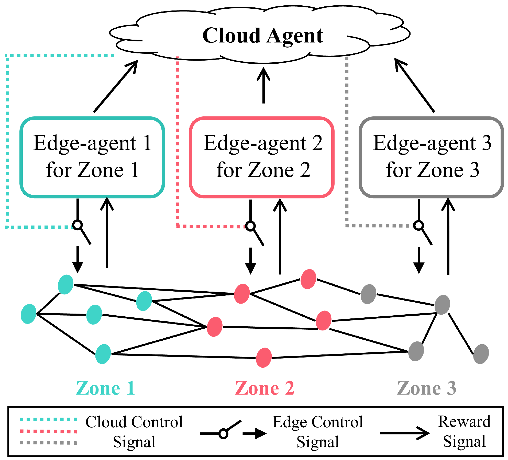
In this section, the decentralized cloud–edge reinforcement learning framework is introduced for the emergency voltage stabilization problem. Cloud agents activate specific edge agents, while the edge agents control their associated loads. The cloud–edge collaborative reinforcement learning formulation for emergency voltage control will be first introduced in this section, including the state, action, and reward settings for both cloud agent and edge agents, respectively; subsequently, the optimization algorithm for training the cloud agent and edge agents, guided surrogate-gradient-based evolutionary random search (GSERS), will be presented; finally, the framework for emergency voltage control based on cloud–edge collaborative reinforcement learning will be introduced.

3.1. Cloud–Edge RL Formulation

Consider a power system divided into a total of N regions with each edge agent corresponds to a region. The set of nodes included in each region is defined as Z n r e g , with  n N + and n N . Given that in complex power systems, there exist non-negligible connections between each region, such as mutual influences of power flows, it is necessary to assign some nodes to multiple regions simultaneously. Formally, the set of these public nodes are defined as Z n p u b . On this basis, we define Z n as the union of all nodes within region n and the public nodes in Z n p u b , i.e.,  Z n = Z n r e g Z n p u b . Its physical meaning is the set of nodes that have a significant influence on region n. In practice, the regional partition { Z n reg } is determined using the electrical centrality-based clustering method of [46], which groups buses according to their effective electrical resistance distances to identify operationally coherent areas that reflect the physical coupling structure of the grid. Alternative approaches such as spectral clustering on the admittance matrix or power transfer distribution factor (PTDF)-based sensitivity partitioning could equally be applied. The public node set Z n pub consists of tie-line endpoint buses whose voltages are materially influenced by power injections in neighboring areas. Including these nodes in each edge agent’s observation set ensures that cross-area coupling effects are explicitly captured without requiring full system observability. The proposed architecture is inherently robust to partition choices, since the cloud coordinator observes the full system state and compensates for any inter-area coordination gaps arising from imperfect partitioning. A formal sensitivity analysis with respect to partition boundary variations is left for future work. Therefore, we introduce the RL formulation for the cloud agent and each edge agent as follows:
(1) RL state: For a power system with region n, the state of cloud agent at time step τ is represented by s τ . Similarly, the state of each edge agent at time step τ is represented by s τ , n . Formally, s τ and s τ , n are represented as follows:
s τ = { ξ τ , η τ }
s τ , n = { ξ τ , n , η τ , n }
where ξ τ denotes the bus voltage magnitudes at monitored locations; η τ denotes the remaining load fractions at controllable buses in the system. Similarly, ξ τ , n and η τ , n denote the corresponding bus voltage magnitudes at monitored locations and the remaining load fractions at controllable buses only included within Z n .
(2) RL action: For a power system with region n, the load reduction control action of cloud agent at time step τ is represented by a τ . Similarly, the load reduction control action of each edge agent at time step τ is represented by a τ , n . Formally, a τ and a τ , n are represented as follows:
a τ = { X n } n = 1 N with X n { T r u e , F a l s e }
a τ , n = μ τ , n
where a τ is a vector of length N composed of Boolean variables X n ; μ τ , n represents the emergency intervention vector, implemented as a continuous load shedding ratio vector over the controllable buses in region n.
(3) RL reward: For a power system with region n, the emergency voltage stabilization reward of cloud agent with respect to policy ϕ is represented by J ( ϕ ) . Similarly, the emergency voltage stabilization reward of each edge agent with respect to policy ϕ n is represented by J n ( ϕ n ) . Formally, J ( ϕ ) and J n ( ϕ n ) are represented as follows:
J ( ϕ ) = τ = τ s τ f R τ
J n ( ϕ n ) = τ = τ s τ f R τ , n
where R τ and R τ , n are the instant reward of cloud agent and each edge agent that detailed in (7). Note that J ( ϕ ) and J n ( ϕ n ) are the sum of immediate rewards.
Remark (Stabilizing Nature of Load Shedding for FIDVR): It is worth emphasizing that, for the FIDVR problem considered in this work, load shedding is by physical nature an inherently stabilizing control action. The root cause of FIDVR is the excessive reactive power absorbed by stalled induction motors following a fault, which prevents bus voltages from recovering after fault clearance [2]. Shedding the stalled motor loads directly eliminates the source of excessive reactive power demand, thereby facilitating voltage recovery regardless of the specific timing or location of the shedding action. Consequently, the coordination decisions made by the cloud–edge framework—determining when, where, and how much load to shed—affect the optimality of the control outcome (i.e., how little load needs to be interrupted to achieve recovery), but not the stability of the voltage recovery process itself. This is a key distinction from other power system control problems where inappropriate control actions could actively worsen system stability. In this problem context, the cloud–edge coordination mechanism cannot introduce new voltage instability by design, and the closed-loop stability of the voltage recovery process is guaranteed by the physical properties of the load shedding action itself.

3.2. Guided Surrogate-Gradient-Based Evolutionary Random Search (GSERS)

Evolutionary strategies borrow ideas from natural selection, where organisms with better traits survive and reproduce over generations. In a similar way, the evolutionary strategies generate populations of randomly changed parameters ϕ j and measure how well each one performs based on total rewards [47]. The algorithm keeps the best candidates from each round and uses their statistical properties to guide the next round of search. This selection-and-variation cycle repeats until the strategy converges to a good solution.
One practical benefit of evolutionary strategies is that they do not rely on the critical backpropagation step needed by derivative-based DRL methods. Instead of computing exact gradients through the derivative backpropagation of the neural network, evolutionary strategies estimate the gradient direction by comparing rewards from many stochastic perturbed parameter sets. This simultaneous stochastic-perturbation approach can be performed in a fully parallel manner, as the computation of different stochastic-perturbation directions is independent from each other, which provides a very efficient speeds-up training. The core RL goal is to minimize the negative expected discounted return:
J ( ϕ ) = E { k = 0 T ρ k k ( s k , π ( s k | ϕ ) ) }
In an evolutionary strategy setup, the parameter ϕ is updated step by step based on estimates of which perturbation direction improves J ( ϕ ) . The problem is that the objective function often has many local minima because it is non-convex, and the optimizer can get stuck before reaching a global solution.
Gaussian smoothing offers a way around this problem. The idea is to average the objective over a range of nearby points so that small bumps in the reward function’s landscape are smoothed out, making the main trends easier to follow. Think of it as blurring a noisy image to see the underlying pattern. With a d-dimensional Gaussian distribution N ( 0 , I d ) , the smoothed objective J ν ( ϕ ) takes the form [48]:
J ν ( ϕ ) = 1 ( 2 π ) d / 2 R d J ( ϕ + ν ϵ ) e 1 2 | | ϵ | | 2 2 d ϵ
where ν controls how much smoothing is applied. If we write the Gaussian density as ζ ( ϵ ) = 1 ( 2 π ) d / 2 e 1 2 | | ϵ | | 2 2 , then the gradient of J ν ( ϕ ) with respect to ϕ can be written as:
ϕ J ν ( ϕ ) = ϕ 1 ( 2 π ) d / 2 R d J ( ϕ + ν ϵ ) e 1 2 | | ϵ | | 2 2 d ϵ = ϕ R d ζ ( ϵ ) J ( ϕ + ν ϵ ) d ϵ = E ϵ N ( 0 , I d ) ϵ | | ϵ | | 2 2 2 J ( ϕ + ν ϵ ) ν = 1 ν E ϵ N ( 0 , I d ) J ( ϕ + ν ϵ ) ϵ ,
This gradient can be seen as an average of directional derivatives along random Gaussian directions:
G = 1 ν M j = 1 M ϵ j [ J ( ϕ + ν ϵ j ) J ( ϕ ) ] ,
For evolutionary strategies to converge well, the variance of the gradient estimate must stay low. The error variance goes as ν 2 / m , where m is the number of samples. One way to reduce the error variance is to use more samples in parallel.
Another way to reduce the error variance is antithetic sampling, which pairs each sample with its mirror image [49]. The logic is simple: when J ( ϕ ) is high for one sample, it tends to be low for the paired sample because they sit on opposite sides of the current point. These opposite values help cancel out noise in the gradient estimate. With M pairs evaluated at ϕ j + = ϕ + ν ϵ j and ϕ j = ϕ ν ϵ j , the gradient estimate becomes:
G = κ 2 ν M j = 1 M ϵ j [ J ( ϕ j + ) J ( ϕ j ) ] ,
where κ is a scaling constant.
Antithetic sampling has its own limits, though. It only reduces variance when the correlation between J ( ϕ j + ) and J ( ϕ j ) is negative. When ϕ varies a lot, the curvature in exponential and logarithmic parts of the objective weakens the cancellation effect [49]. In practical terms, the paired samples stop producing opposite reward values, and the variance stays high. As a result, evolutionary strategies can still have difficulties with converging, especially for large problems with many parameters.
We address these issues with the guided surrogate-gradient-based evolutionary random search (GSERS) algorithm. The key idea is to combine the robustness of evolutionary search with lower-variance gradient estimates estimated from past optimization steps [50]. By keeping track of previous surrogate gradients, the algorithm builds a low-dimensional subspace that captures the main directions of improvement. Future perturbations are then concentrated in this low-dimensional subspace, which is more likely to contain useful search directions. Even if we cannot compute ϕ J ν ( ϕ ) directly, the history of past updates tells us something useful about how J ( ϕ ) behaves. The accumulated gradient vectors form a kind of map of the objective landscape. By focusing the random samples inside this guided subspace, we cut down the variance of the search directions substantially. This helps GSERS scale better and converge more reliably than standard evolutionary methods while still giving unbiased gradient estimates.
Suppose we have surrogate gradient vectors from each iteration of the optimization. By collecting these gradients over the last h iterations, we form a subspace that captures the recent history of improvement directions. This subspace has an orthonormal basis U of size d × h , where U T U = I h . GSERS uses this subspace by changing the distribution of the perturbation ϵ j from the standard Gaussian N ( 0 , I d ) to a guided Gaussian N ( 0 , Λ ) , with  Λ defined as:
Λ = δ 2 I d + ( 1 δ ) 2 U U T
In Equation (19), the parameter δ sets the trade-off between random exploration and guided search using the surrogate gradient subspace. When δ = 1 , GSERS acts like a plain evolutionary strategy with no guidance, sampling perturbations uniformly in all directions. When δ = 0 , all perturbations are sampled within the guided subspace, which may miss good directions outside that subspace. We use δ = 0.5 in our algorithms to make the exploration and exploitation balanced. Under this new distribution, each perturbation ϵ j is sampled as:
ϵ j = δ ϵ ( 1 ) + ( 1 δ ) ϵ ( 2 ) ,
where ϵ ( 1 ) N ( 0 , I d ) and ϵ ( 2 ) N ( 0 , I h ) . The full procedure of the GSERS is shown in Algorithm 1.
Algorithm 1 Guided Surrogate-gradient-based Evolutionary Random Search (GSERS).
  1:
Input Parameters: ( E ), where E denotes the system environment;
  2:
Initial Configuration: ( ϕ , s 0 , η , ν ), where ϕ represents policy parameters; s 0 denotes initial system state; η is the step size; ν controls perturbation magnitude;
  3:
while training incomplete do
  4:
   Generate guided perturbations: ϵ N ( 0 , Λ )
  5:
   Formulate parameter variations: ϕ + = ϕ + ν ϵ , ϕ = ϕ ν ϵ
  6:
   Initialize environment state, set time index k = 0
  7:
   for each parameter set ϕ + and ϕ  do
  8:
     while  k T  do
  9:
         a k ϕ + ( s k )   alternatively a k ϕ ( s k )
10:
         s ( k + 1 ) E ( a k ) , k k + 1
11:
     end while
12:
     Compute trajectory return J
13:
   end for
14:
   Estimate G via Equation (18)
15:
   Execute parameter update: ϕ ϕ η G
16:
end while
17:
Output: Optimized policy parameters ϕ

3.3. Cloud–Edge Collaborative DRL Algorithm

This section presents a distributed learning framework for emergency voltage control using the GSERS method described in Section 3.2. The main idea is to allow each area of the power grid to learn its own control policy for load shedding. For this setup to work, every area must contain a sufficient number of controllable loads so that the RL agent has a meaningful action space to explore. If an area has too few controllable resources, the  learning problem becomes trivial or poorly defined.
An edge agent operating within a single area alone, however, cannot observe what is happening elsewhere in the grid. Power flows across tie lines that link the areas together, meaning that actions taken in one area can affect the bus voltages in neighboring areas. Without some form of coordination, the edge agents of different areas may work at cross purposes, with one area shedding too much load while another sheds too little. To address this problem, a cloud-level controller sits above the edge agents and decides when and how to activate them, steering the overall system toward a globally optimal outcome. Figure 2 shows this cloud–edge layout.
Each edge agent of an area is treated as a separate DRL agent with its own environment and operating limits. During the distributed training phase, every edge agent runs GSERS over many episodes and learns a local policy for voltage recovery within its own area. The  edge policies are trained on fault scenarios that occur within each area, so each agent becomes an expert in its own territory. Once the edge policies are trained, the cloud agent learns how to coordinate them by observing the joint behavior of all edge agents acting together. This two-level setup allows the cloud agent to determine which edge agents should take load shedding control actions and in what time sequence, bringing the combined behavior of multiple edge agents close to a system-wide optimum. The complete training loop is given in Algorithm 2.
Algorithm 2 Cloud–Edge Collaborative Training Framework.
  1:
System Parameters: ( E , N , N c , N e ), where E denotes the complete power system environment containing N regional partitions; N c and N e specify iteration counts for cloud-level and edge-level training respectively;
  2:
Initial Setup: { ϕ j } j = 1 N , ϕ c , where { ϕ j } j = 1 N represents the policy collection for edge agents; ϕ c denotes the cloud agent’s coordination policy;
  3:
while convergence not achieved do
  4:
   Generate regional environment collection: E = { E j } j = 1 N
  5:
   for Edge training cycle n e = 0 to N e  do
  6:
     for Regional index j = 1 to n do
  7:
         ϕ j Algorithm 1 ( E j );
  8:
        Refresh policy collection Φ ;
  9:
     end for
10:
   end for
11:
   for Cloud training cycle n c = 0 to N c  do
12:
      ϕ c Algorithm 1 ( E );
13:
   end for
14:
end while
15:
Output: Cloud coordination policy ϕ c ; Edge policy collection Φ

4. Results

4.1. Test System and Simulation Setup

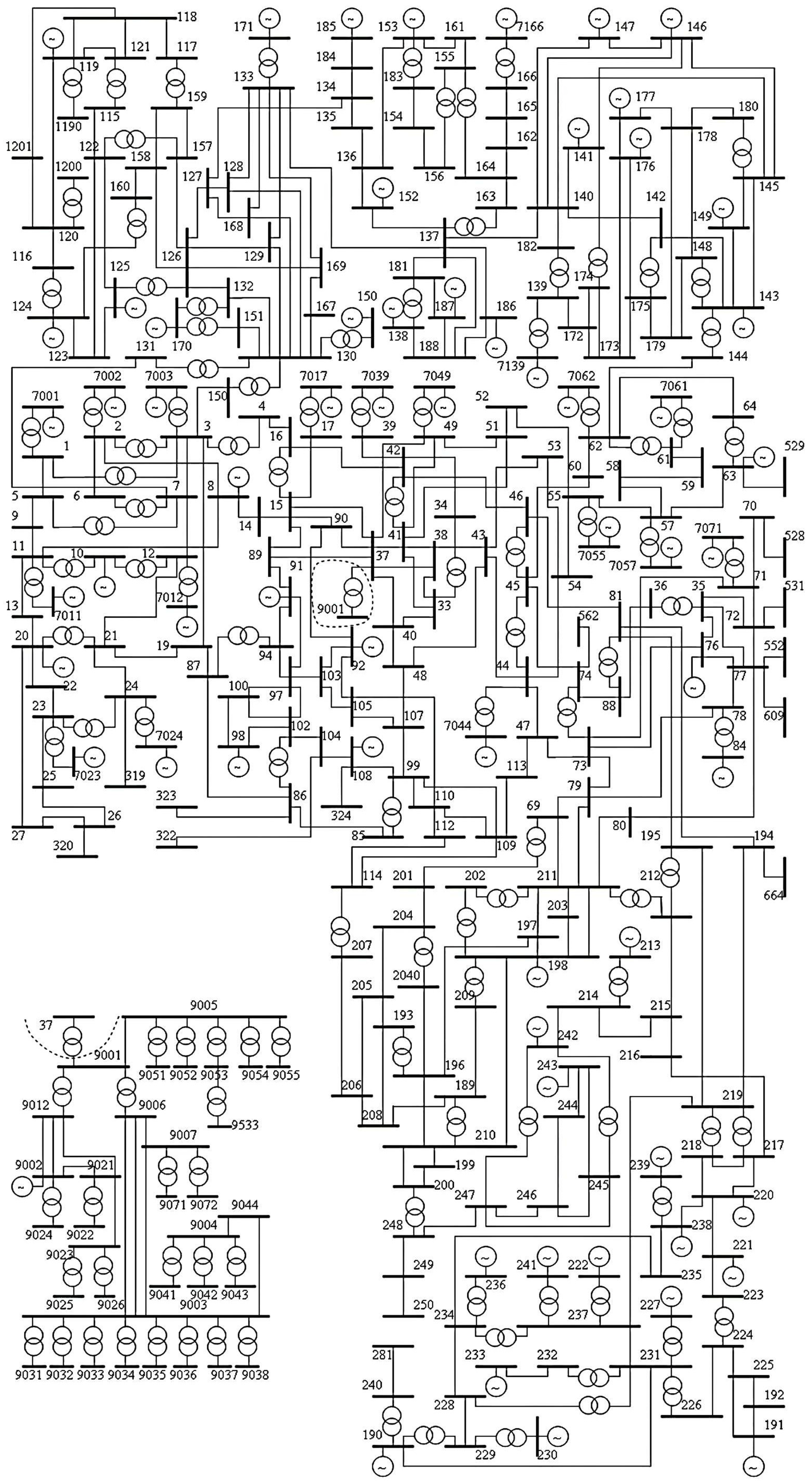
The simulation is performed on the IEEE 300-bus test system [51], as illustrated in Figure 3. This system was deliberately chosen over smaller benchmarks for two reasons. First, the IEEE 300-bus system is large enough to expose the scalability limitations of centralized DRL: the high-dimensional observation and action spaces, combined with the complex dynamics of the large-scale grid, require a substantially larger policy network and a much broader set of training scenarios, leading to prohibitive training times under the centralized approach. A smaller system, such as the IEEE 39-bus or IEEE 118-bus system, would not adequately stress-test these scalability properties, as a centralized DRL agent can be trained on such systems within a manageable time. Second, the IEEE 300-bus system is a well-established and widely adopted benchmark in the power systems research community, ensuring that our results are reproducible and can be meaningfully compared with existing literature. The network topology can be partitioned into three separate operational zones as shown in [46]. Within each zone, we select specific buses to introduce the fault during the training. In Area 1, fault is applied at buses 2, 33, 59, 67, 45, 18, 87, 22, denoted as the fault bus subset F s e t 1 ; in Area 2, fault is applied at buses 110, 132, 123, 128, 135, 140, 154, 161, and 21, denoted as the fault bus subset F s e t 2 ; and for Area 3, fault is applied at buses 190, 232, 205, 220, 217, 228, 231, denoted as the fault bus subset F s e t 3 .
The proposed Cloud–Edge Collaborative DRL framework was implemented and validated on a hardware setup designed to reflect a realistic deployment scenario for large-scale power grid emergency control. The hardware architecture consists of two layers, corresponding to the cloud level and the edge level of the proposed framework, respectively.
At the cloud level, a centralized server equipped with an Intel Xeon Gold 6258R processor (28 cores, 2.7 GHz base frequency), 256 GB of DDR4 RAM, and an NVIDIA A100 GPU (40 GB HBM2 memory) is used to host the cloud supervisory DRL agent. This server is responsible for coordinating the edge agents by aggregating their updated policies and executing the cloud-level GSERS training. The high memory capacity and multi-core architecture of the cloud server allow it to handle the global system observations and run the coordination training efficiently.
At the edge level, three edge computing nodes are deployed, one for each operational zone of the IEEE 300-bus system. Each edge node is equipped with an Intel Core i7-1185G7 processor (4 cores, 3.0 GHz base frequency) and 32 GB of DDR4 RAM. These edge nodes are representative of the computing hardware that would typically be available at regional grid control centers. Each edge node runs its own local DRL agent and executes the area-specific GSERS training independently using fault scenarios local to its assigned zone.
The cloud server and edge nodes communicate over a dedicated local area network (LAN) with a bandwidth of 1 Gbps. In the training phase, communication between the cloud and edge layers is limited to the transmission of updated policy network parameters (i.e., neural network weights), which have a small data footprint compared to raw measurement data. In the inference (deployment) phase, the cloud agent transmits Boolean activation signals to the edge agents, and the edge agents return their local reward signals to the cloud agent for monitoring purposes. This lightweight communication design ensures that the cloud–edge framework remains robust to communication delays and is well-suited for real-world deployment.
The power system simulations were carried out using the dynamic simulation method described in reference [53,54]. All training and testing experiments were conducted on the hardware described above, with edge-level training processes running in parallel across the three edge nodes simultaneously.

4.2. Test Results

Prior to demonstrating the effectiveness of the proposed Cloud–Edge Collaborative Deep Reinforcement Learning framework, we establish baselines by evaluating two alternative approaches as comparison methods: (1) a full-scale centralized training approach, which uses a training procedure described in [55], and (2) a purely decentralized area-wise policy approach, which uses a training procedure described in [56]. For the centralized full-scale model, we construct a policy network featuring an LSTM layer with 64 hidden units followed by a fully connected layer with 64 units. For the purely decentralized area-wise policy approach, each of the three areas is assigned a policy network featuring an LSTM layer with 16 hidden units followed by a fully connected layer with 16 units.
For both the centralized and the decentralized approaches, the fault bus set is the union of the three predefined fault bus subsets F s e t 1 F s e t 2 F s e t 3 . These faults are applied with three varying durations: 0.05, 0.1, and 0.2 s. Upon completing the training, the resulting policies are tested against a variety of grid faults.
Subsequently, we implement the Cloud–Edge Collaborative Deep Reinforcement Learning framework. We deploy the control architecture depicted in Figure 2 and subject it to the same fault scenarios used for training and testing with the centralized and decentralized methods. Both the edge-layer policy networks and the cloud-level coordinator network are structured with 16 hidden units in the LSTM layer and 16 units in the fully connected layer, aiming to learn optimized control strategies. We adhere to the protocol detailed in Section 3 to train the edge controller policies for the three areas, utilizing the parameters listed in Table 1. The cloud coordinator is assigned a larger number of search directions (24 vs. 18) and top candidates (10 vs. 8) compared to the edge agents, as it must navigate a higher-dimensional coordination policy space that spans all three areas of the grid simultaneously, requiring broader exploration to converge to a reliable coordination strategy.
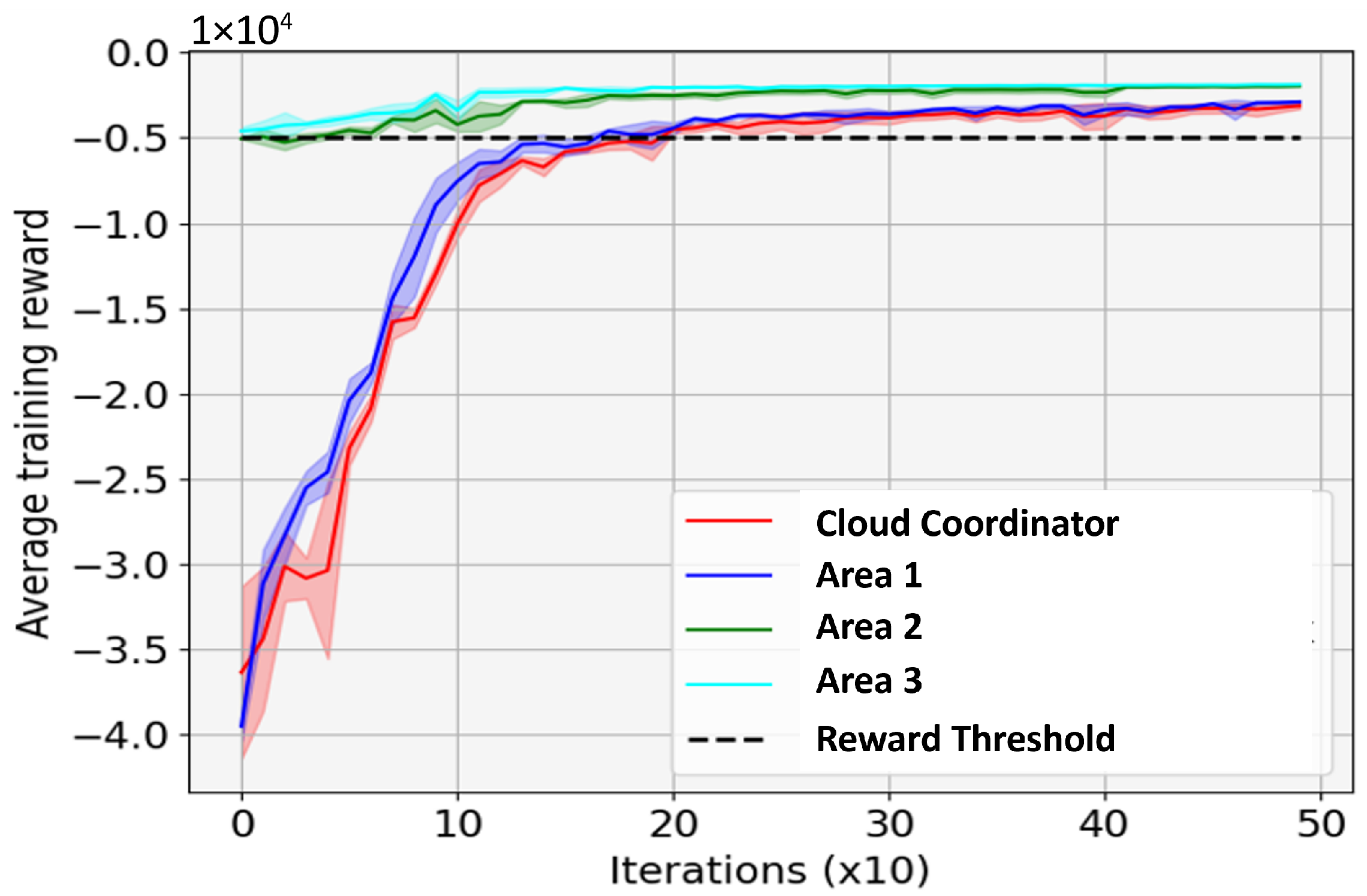
Figure 4 illustrates the learning curve during the Cloud–Edge Collaborative DRL training process, plotting average rewards over all fault rollouts at the end of every 10 iterations. To verify reproducibility, the training was conducted using multiple random seeds. The area-wise decentralized edge training involved three distinct training processes for the individual area policies. Simultaneously, lower-level edge policy updates are integrated via Algorithm 2 to train the high-level cloud coordinating RL agent. This agent learns to intelligently select lower-level edge policies based on the fault’s impact on the grid. The coordinator generates rollouts by randomly selecting a fault bus from the training set of each area. Figure 4 also depicts the cloud coordinator’s training progress. A comparison with the centralized training is shown in Table 2, which demonstrates that the training time is reduced by approximately 90%, confirming the computational scalability of the proposed Cloud–Edge DRL framework relative to the fully centralized approach.
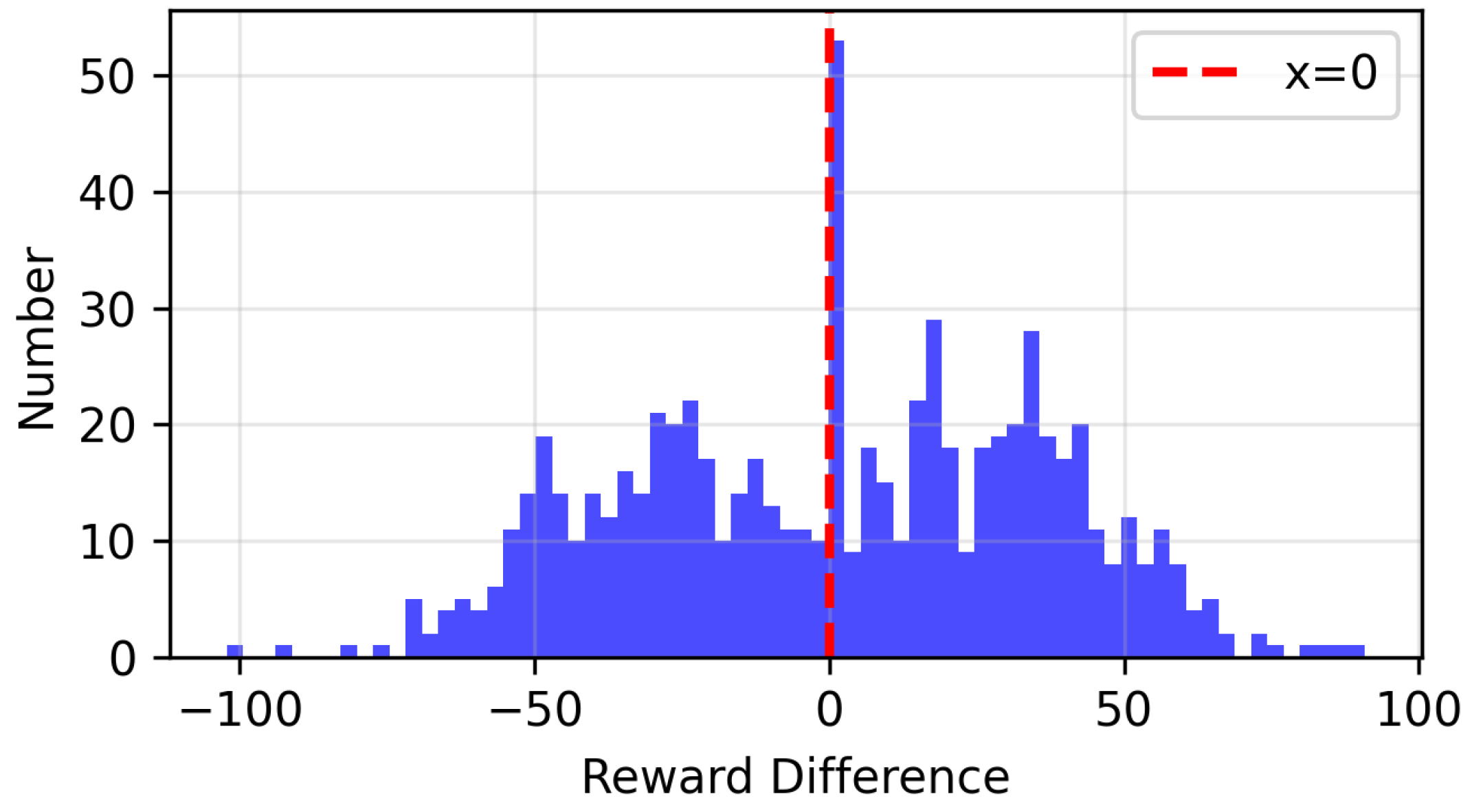
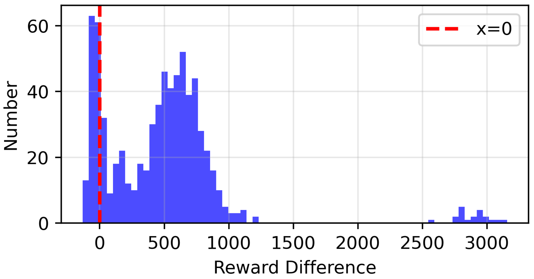
To validate the performance of the Cloud–Edge policies quantitatively, we compare the rewards for all test cases among the proposed Cloud–Edge Collaborative DRL method, the fully centralized DRL method, and the fully decentralized method. We compute the reward differences (i.e., the reward of the Cloud–Edge method minus that of the fully centralized method) for all test cases. A positive value indicates that the Cloud–Edge method performs better for the corresponding test scenario with respect to the reward defined by Equation (7), and vice versa. Figure 5 shows the reward difference histogram between the proposed Cloud–Edge method and the fully centralized method. As seen in Figure 5, the proposed Cloud–Edge method achieves comparable performance to the fully centralized method, as the counts of positive and negative reward differences are nearly equal and symmetrically distributed, confirming that the Cloud–Edge framework matches centralized control performance while drastically reducing training cost.
Figure 6 shows the reward difference histogram between the proposed Cloud–Edge method and the fully decentralized method. As seen in Figure 6, the proposed Cloud–Edge method achieves approximately 80% better reward performance compared to the fully decentralized approach across all test fault scenarios, clearly demonstrating the critical benefit of the cloud-level coordination mechanism. It is also worth noting that approximately 24 counts correspond to reward differences around the value 3000. This indicates that for these 24 test scenarios, the fully decentralized method failed to restore the system voltage to its normal value within 1.5 s of fault clearance, incurring a large negative reward penalty, whereas the proposed Cloud–Edge method successfully restored the system voltage within the required timeframe.
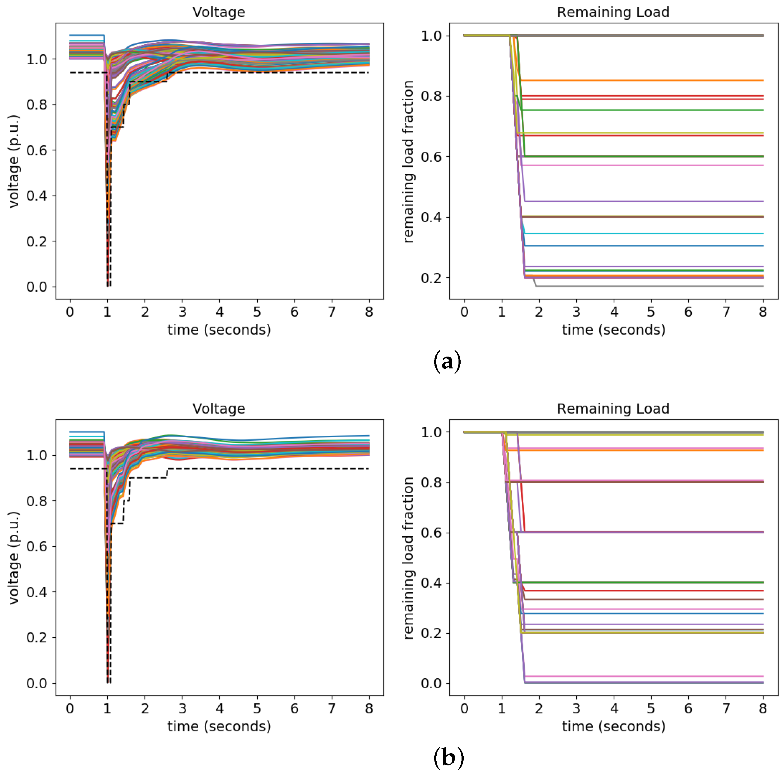
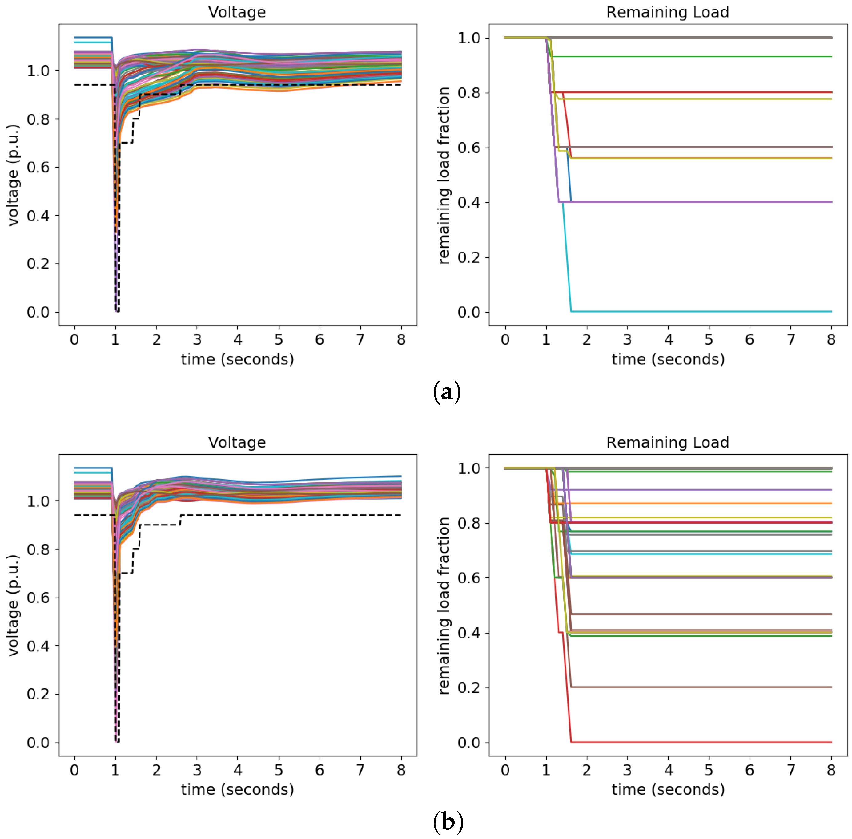
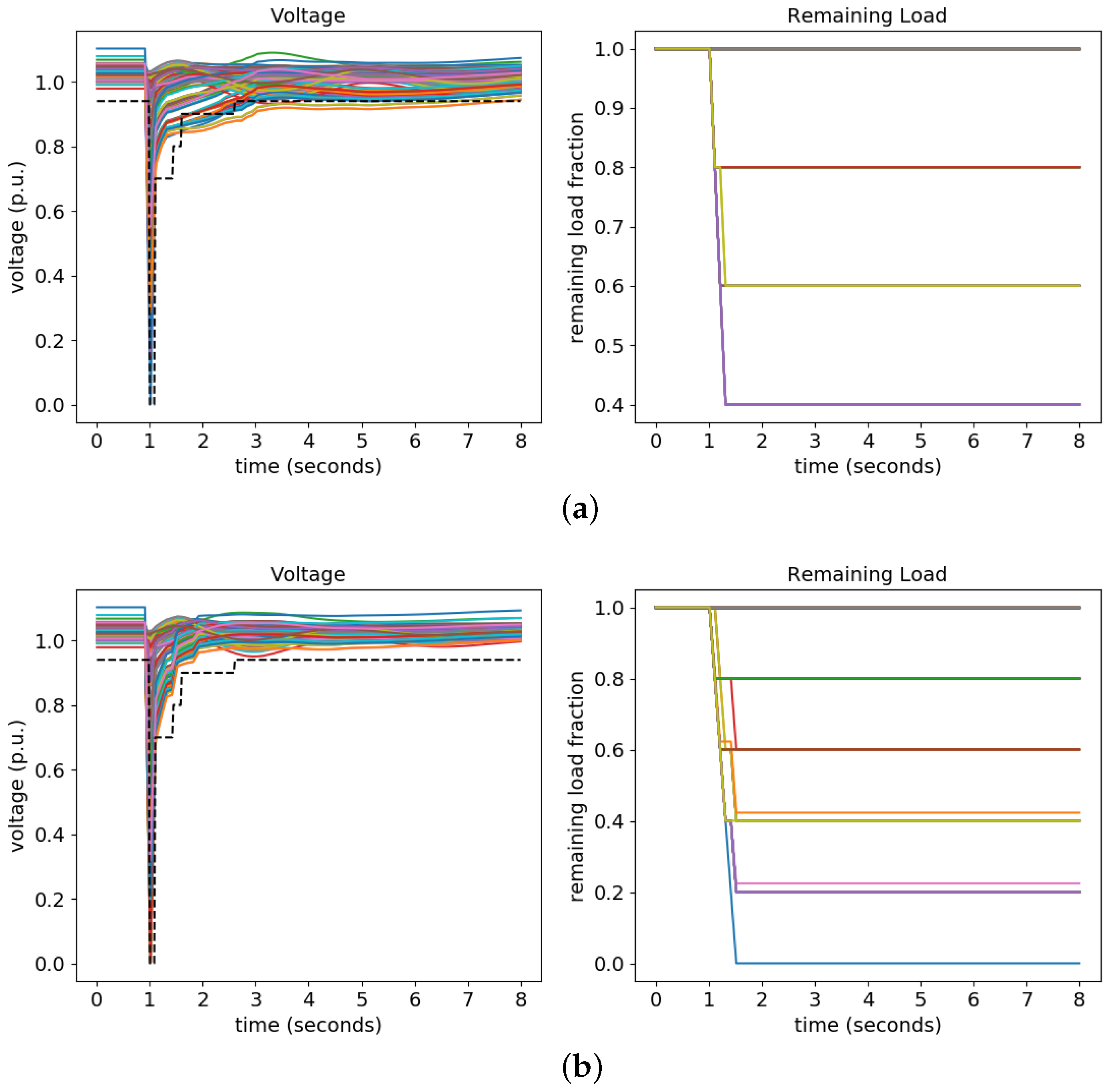
To further illustrate the performance of the proposed Cloud–Edge method and compare it with the fully centralized and decentralized methods, we present detailed system voltage recovery curves and load shedding actions for several specific test scenarios under each approach. Figure 7a depicts a case where the centralized policy fails to restore voltages across all buses following a fault at bus 163 with a fault duration of 0.1 s. Specifically, the voltage of some buses in the system falls below the voltage recovery criterion defined in Figure 1 during the recovery period (particularly around 1.8 to 2.5 s). This outcome suggests that the non-collaborative centralized policy design requires a significantly larger policy network with more parameters to achieve acceptable performance levels. However, scaling up the policy network creates a computational bottleneck for large power grids, and the full-scale centralized training process required 96.37 h to complete. By comparison, Figure 7b shows that the proposed Cloud–Edge Collaborative method successfully keeps the system voltage above the recovery criterion defined in Figure 1 throughout the entire voltage recovery period. This detailed comparison demonstrates the Cloud–Edge Collaborative DRL framework’s ability to coordinate edge agents across different areas, yielding performance that surpasses the centralized design. Figure 8 presents another test case comparison between the centralized policy and the proposed Cloud–Edge Collaborative method, which further demonstrates that the centralized policy fails to satisfy the voltage recovery criterion during the recovery period, while the proposed method succeeds.
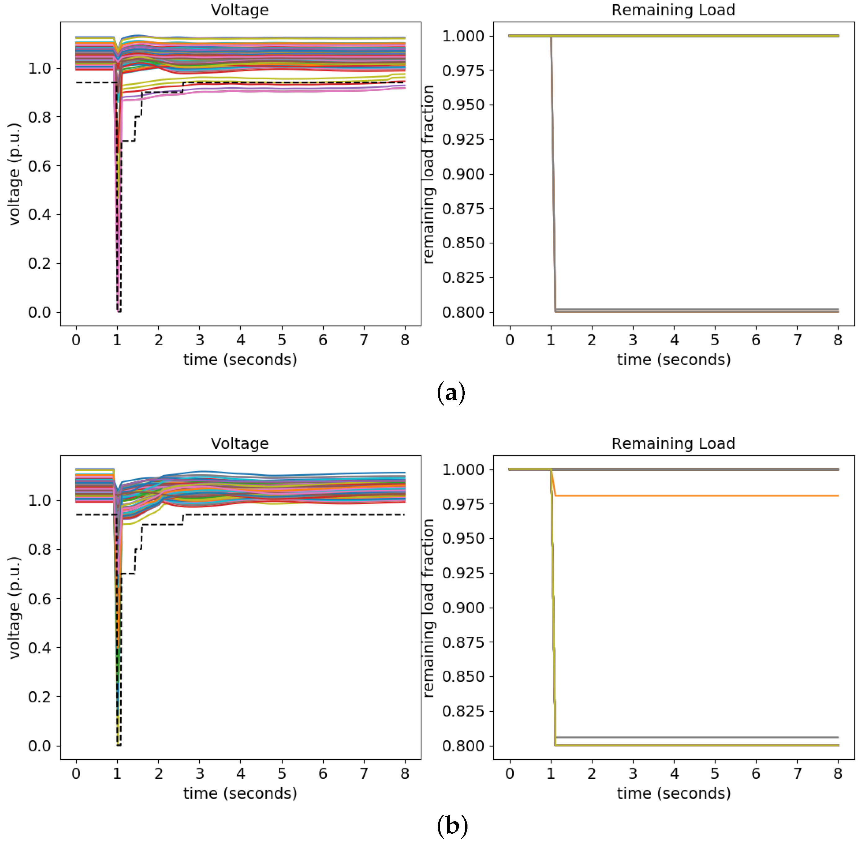
Figure 9a depicts a failure case where the fully decentralized policy fails to restore voltages across all buses following a fault at bus 52 with a fault duration of 0.1 s, as the voltages of some buses remain below the recovery criterion defined in Figure 1 even 4 s after fault clearance. This outcome indicates that the fully decentralized policy design cannot guarantee complete voltage recovery across the system, as it lacks coordination between different areas. Figure 9a clearly illustrates that control actions confined to Area 1 alone fail to improve the grid’s dynamic response, even when the fault originates within Area 1 (fault at bus 52 with a 0.1 s duration). This is because the fault occurs near the boundary of Areas 1 and 2, causing FIDVR issues at buses in both areas simultaneously, which the non-collaborative decentralized policies are unable to handle through coordination. By comparison, Figure 9b shows that the proposed Cloud–Edge Collaborative method successfully restores the system voltage, with bus voltages remaining above the recovery criterion defined in Figure 1 throughout the recovery period. Note that this test scenario corresponds to one of the 24 counts with reward differences around 3000 in Figure 6, where the fully decentralized method failed to restore the system voltage within 1.5 s of fault clearance and thus incurred a large negative reward penalty. This detailed comparison demonstrates the Cloud–Edge Collaborative DRL framework’s ability to coordinate edge agents across different areas, yielding performance that significantly surpasses the fully decentralized method. Figure 10 presents another test case comparison between the fully decentralized policy and the proposed Cloud–Edge Collaborative method, which further confirms that the fully decentralized policy fails to restore system bus voltages to meet the recovery criterion, while the proposed method succeeds.
The test results provide empirical evidence of bounded and stable closed-loop behavior under the proposed cloud–edge collaborative DRL framework. The trained policies were evaluated on fault scenarios with randomly selected fault durations in the range of 0.1 s to 0.3 s at multiple grid locations, including fault buses deliberately withheld from the training set to assess the generalization of the learned policies to previously unseen operating conditions. Across all tested scenarios, the cloud–edge framework successfully recovered bus voltages above the required thresholds within the prescribed time windows defined by the transient voltage recovery criterion shown in Figure 1. No unbounded or divergent voltage trajectory was observed under the proposed control framework, which is consistent with the analytical argument presented in Section 2 that load shedding is an inherently stabilizing action for the FIDVR problem. Furthermore, the reward difference histogram in Figure 5 confirms that the proposed method achieves comparable performance to the fully centralized approach across the full distribution of test cases, with no systematic failure modes or destabilization events observed, providing further empirical support for the robustness of the learned coordination and edge-level policies. We acknowledge that formal closed-loop stability certificates—analogous to Lyapunov-based guarantees in classical control theory —are not yet available for general DRL-based controllers and remain an important open problem in the field [57]. Extending the proposed framework with formal safety guarantees, for example through the integration of control barrier functions or safe reinforcement learning techniques, is identified as a valuable direction for future research.
It is important to acknowledge that the proposed cloud–edge collaborative DRL framework does not represent a completely decentralized solution. We have integrated a cloud-level coordinator that maintains limited interaction with the grid’s lower layers. Furthermore, the neural networks employed in both the centralized and collaborative approaches introduce significant non-linearity into the closed-loop dynamics. This complexity makes direct reward comparisons nuanced, as the conventional assumption that centralized designs inherently outperform distributed ones may not strictly apply in these machine learning paradigms. However, our empirical results validate that the cloud–edge collaborative deep reinforcement learning framework achieves average performance levels close to the centralized approach, and in certain fault scenarios, may even yield superior rewards.

4.3. Computational Cost Assessment

To assess the real-time feasibility of the proposed cloud–edge collaborative DRL framework, we measured the average wall-clock inference time for both the edge agents and the cloud coordinator per control cycle. All measurements were performed on the hardware described in Section 4.1, with each timing result averaged over 1000 inference calls to ensure statistical reliability. The results are summarized in Table 3.
All edge agents achieve an average inference time well below 12 ms per control cycle, which is significantly shorter than the required emergency response window of several seconds for FIDVR mitigation. Note that in the proposed architecture, the three edge agents execute their inference steps in parallel on their respective edge computing nodes simultaneously, so the effective edge-level latency per control cycle is equal to the inference time of a single edge agent rather than the sum of all three.
Beyond the neural network inference time, the additional overhead introduced by the cloud coordinator involves two components: the coordinator’s own inference step and the cloud–edge communication latency. As shown in Table 3, the cloud coordinator’s inference time is comparable to that of the edge agents, owing to its similarly compact network architecture. Regarding communication overhead, the proposed framework is specifically designed to minimize inter-layer data transmission. In the downlink direction (cloud to edge), the coordinator transmits only a vector of N = 3 Boolean activation signals per control cycle—one per grid area—representing a payload of just 3 bits. In the uplink direction (edge to cloud), each edge agent transmits its local state observation vector, consisting of bus voltage magnitudes and load fractions. Table 4 summarizes the communication payload and estimated transmission latency for a standard 1 Gbps LAN connection.
As evident from Table 4, the communication overhead is negligible compared to both the inference time and the control cycle duration, confirming that the cloud–edge communication design does not impose any real-time bottleneck. The total latency per control cycle—comprising parallel edge inference, cloud coordinator inference, and communication—remains well within the required emergency response window for FIDVR control, validating the real-time feasibility of the proposed framework. We note that the present study is simulation-based and the communication latency values reported above are theoretical estimates based on payload size. A full hardware-in-the-loop validation under realistic wide-area network conditions, where latency jitter and packet loss may be relevant, is identified as an important direction for future research.

5. Future Work Discussion

Several promising directions remain for future research. First, the current framework assumes that communication between the cloud coordinator and the edge agents is instantaneous and reliable. In practice, however, real-world deployments of cloud–edge architectures are subject to both input-side delays—arising from measurement transmission latencies between field sensors and edge nodes—and parametric delays in the cloud-to-edge control signal propagation. Such delays can degrade the performance of the trained DRL policies, as the agents may act on outdated state observations or receive coordination signals after the optimal intervention window has passed. Future work will investigate the incorporation of explicit delay models into the MDP formulation, for example by augmenting the state representation with delayed observation buffers [58], or by training the agents under randomized delay conditions to improve robustness to variable communication latencies in realistic grid communication infrastructures.
Second, the current framework does not explicitly account for regional uncertainties in power system operating conditions. In practice, load behavior varies significantly across regions and time periods, renewable generation introduces stochastic variability that is difficult to characterize precisely, and grid topology may change due to planned switching or unexpected outages. These sources of uncertainty can cause the learned edge policies to encounter operating conditions that differ substantially from the training distribution, potentially degrading voltage recovery performance. Future extensions will explore the integration of robust reinforcement learning formulations [59] and distributionally robust optimization techniques into the GSERS training process, enabling the edge agents to learn policies that are explicitly resilient to regional parametric uncertainties and distributional shifts in fault scenarios.
Third, the current work models induction motor loads using a fixed parametric representation. Future work will investigate the sensitivity of the trained policies to variations in motor model parameters—such as rotor resistance, inertia constants, and load composition ratios—across different regions of the grid. This will help quantify the robustness margins of the proposed framework and guide the design of adaptive retraining strategies for edge agents operating in regions with heterogeneous or time-varying load characteristics.
Finally, while this work focuses on the FIDVR problem as the primary application, the proposed cloud–edge collaborative DRL architecture is general and can in principle be extended to other power system emergency control tasks, such as frequency regulation under large generation loss events and transient stability control following severe network faults. Exploring these extensions, as well as the combination of the cloud–edge framework with physics-informed neural network architectures [60] that can better generalize across operating conditions, represents a rich avenue for future investigation.

6. Conclusions

In this study, we proposed a scalable reinforcement learning methodology for automated emergency voltage control via load shedding. By leveraging the inherent interconnected topology of power grids, we engineered a Cloud–Edge Collaborative Deep Reinforcement Learning framework. In this architecture, edge-level RL agents are trained in a decentralized, area-specific manner, while a high-level cloud agent is trained to intelligently synchronize and oversee the load shedding maneuvers executed by the edge agents. By incorporating modularity into the training phase, this design demonstrates the ability to train sufficiently optimized policies significantly faster than full-scale centralized counterparts. Our analysis confirms that while independent, area-specific decentralized policies may struggle to fully restore bus voltages following severe faults, the intervention of the cloud-level coordinator effectively manages these agents to guarantee voltage stability during emergency conditions. Quantitative evaluation on the IEEE 300-bus system demonstrates three key advantages of the proposed framework. First, the cloud–edge collaborative training achieves approximately 90% reduction in training time compared to the fully centralized approach (9.59 h vs. 96.37 h), confirming its superior scalability to large power grids. Second, the proposed method achieves comparable voltage recovery performance to the fully centralized approach, with the reward difference histogram showing an approximately equal distribution of positive and negative reward differences across all test fault scenarios. Third, the proposed method significantly outperforms the fully decentralized approach, achieving approximately 80% better reward performance, which directly validates the effectiveness of the cloud-level coordination mechanism in resolving the inter-area voltage recovery challenges that purely decentralized agents fail to address. Future research will focus on exploring efficient design variations within multi-agent systems and further refining collaborative frameworks.

Author Contributions

Conceptualization, D.Y., B.C. and R.H.; methodology, D.Y.; software, D.Y. and J.W.; validation, D.Y., J.W. and Y.Z.; writing, D.Y. and R.H.; visualization, Y.Z. and X.T.; supervision, D.Y. and R.H.; project administration, D.Y. and R.H. All authors have read and agreed to the published version of the manuscript.

Funding

This research was funded by Hainan Provincial Natural Science Foundation of China, project number 525QY911.

Data Availability Statement

The original data (code) presented in the study are openly available in https://github.com/Henry-cloud-c/coordinatedRL.git (accessed on 9 March 2026).

Conflicts of Interest

Author Dongyang Yang, Bing Cheng, Jisi Wu, Yunan Zhao, Xingao Tang were employed by the company Hainan Power Grid Co., Ltd. The remaining authors declare that the research was conducted in the absence of any commercial or financial relationships that could be construed as a potential conflict of interest.

Nomenclature

Abbreviations
DRLDeep Reinforcement Learning
FIDVRFault Induced Delayed Voltage Recovery
GSERSGuided Surrogate-gradient-based Evolutionary Random Search
MDPMarkov Decision Process
MPCModel Predictive Control
RLReinforcement Learning
UVLSUnder Voltage Load Shedding
Parameters and Variables
L ( · ) objective function
ξ τ , ξ τ m i n , ξ τ m a x dynamic state vector and the corresponding bounds
η τ , η τ m i n , η τ m a x algebraic state vector and the corresponding bounds
μ τ , μ τ m i n , μ τ m a x control actions and the corresponding bounds
ω τ system fault or disturbance
τ , τ s , τ f time index, start/end time of the emergency control window
h ( · ) , q ( · ) differential and algebraic equations of the system
Ω τ observation at time τ
V τ bus voltage magnitudes in Ω τ
P L τ remaining load fractions at controllable buses
K h historical window size
S τ stacked state of RL
R τ , R τ , n cloud/edge instant reward of RL at time τ
V k ( τ ) voltage at bus k
Δ V k ( τ ) voltage shortfall term
Δ P m ( τ ) per-unit load shed at bus m at time τ
U p e n penalty for invalid shedding actions
α 1 , α 2 , α 3 reward weights
τ f c fault clearing time
M large negative reward penalty constant
τ m a x horizon length
λ discount factor
n , N region index and number of regions
Z n r e g the set of nodes included in each region
Z n p u b public nodes shared across regions
Z n the union of all nodes within region n
s τ , s τ , n cloud/edge agent states
ξ τ , n , η τ , n regional dynamic/algebraic states
a τ , a τ , n cloud/edge action vector
X n activation indicator for region n
ϕ cloud/edge policies
J ( ϕ ) , J n ( ϕ n ) cloud/edge returns as sum of immediate rewards
ν perturbation magnitude
ϵ , ϵ j Gaussian perturbation directions
ρ , π ( · ) discount factor and policy distribution
J ν ( ϕ ) Gaussian-smoothed objective
ζ ( ϵ ) Gaussian density
I d , I h identity matrices
G gradient estimation
κ scaling constant
Msample count
U orthonormal basis of surrogate-gradient subspace
Λ guided covariance
δ exploration–guidance trade-off
E j , E (regional) environment simulator
T , η rollout length and step size in Algorithm 1
N c , N e cloud-level / edge-level training iterations
ϕ c cloud coordination policy
Φ Edge policy collection
F s e t 1 , F s e t 2 fault bus subsets used for training

References

  1. Adhikari, S.; Schoene, J.; Gurung, N.; Mogilevsky, A. Fault Induced Delayed Voltage Recovery (FIDVR): Modeling and Guidelines. In 2019 IEEE Power & Energy Society General Meeting (PESGM); IEEE: Atlanta, GA, USA, 2019; pp. 1–5. [Google Scholar]
  2. Van Cutsem, T.; Vournas, C. Voltage Stability of Electric Power Systems; Springer Science & Business Media: Berlin/Heidelberg, Germany, 2007. [Google Scholar]
  3. Australian Energy Market Operator. Black System South Australia 28 September 2016; Australian Energy Market Operator Limited: Melbourne, VIC, Australia, 2017. [Google Scholar]
  4. Sun, H.; Guo, Q.; Qi, J.; Ajjarapu, V.; Bravo, R.; Chow, J.; Li, Z.; Moghe, R.; Nasr-Azadani, E.; Tamrakar, U.; et al. Review of Challenges and Research Opportunities for Voltage Control in Smart Grids. IEEE Trans. Power Syst. 2019, 34, 2790–2801. [Google Scholar] [CrossRef] [Scilit]
  5. Dong, Y.; Xie, X.; Wang, K.; Zhou, B.; Jiang, Q. An Emergency-Demand-Response Based Under Speed Load Shedding Scheme to Improve Short-Term Voltage Stability. IEEE Trans. Power Syst. 2017, 32, 3726–3735. [Google Scholar] [CrossRef] [Scilit]
  6. Amraee, T.; Ranjbar, A.; Feuillet, R. Adaptive under-voltage load shedding scheme using model predictive control. Electr. Power Syst. Res. 2011, 81, 1507–1513. [Google Scholar] [CrossRef] [Scilit]
  7. Chakraborty, R.; Chakrabortty, A.; Farantatos, E.; Patel, M.; Hooshyar, H.; Darvishi, A. Hierarchical frequency and voltage control using prioritized utilization of inverter based resources. Int. J. Electr. Power Energy Syst. 2023, 144, 108527. [Google Scholar] [CrossRef] [Scilit]
  8. Jin, L.; Kumar, R.; Elia, N. Model Predictive Control-Based Real-Time Power System Protection Schemes. IEEE Trans. Power Syst. 2010, 25, 988–998. [Google Scholar] [CrossRef] [Scilit]
  9. Genc, I.; Diao, R.; Vittal, V.; Kolluri, S.; Mandal, S. Decision tree-based preventive and corrective control applications for dynamic security enhancement in power systems. IEEE Trans. Power Syst. 2010, 25, 1611–1619. [Google Scholar] [CrossRef] [Scilit]
  10. Matavalam, A.R.R.; Ajjarapu, V. PMU-Based Monitoring and Mitigation of Delayed Voltage Recovery Using Admittances. IEEE Trans. Power Syst. 2019, 34, 4451–4463. [Google Scholar] [CrossRef]
  11. Zhang, J.; Lu, C.; Fang, C.; Ling, X.; Zhang, Y. Load shedding scheme with deep reinforcement learning to improve short-term voltage stability. In Proceedings of the 2018 IEEE Innovative Smart Grid Technologies-Asia (ISGT Asia); IEEE: Piscataway, NJ, USA, 2018; pp. 13–18. [Google Scholar]
  12. Huang, R.; Chen, Y.; Yin, T.; Li, X.; Li, A.; Tan, J.; Huang, Q. Accelerated Deep Reinforcement Learning Based Load Shedding for Emergency Voltage Control. arXiv 2020, arXiv:2006.12667. [Google Scholar] [CrossRef] [Scilit]
  13. Mnih, V.; Kavukcuoglu, K.; Silver, D.; Graves, A.; Antonoglou, I.; Wierstra, D.; Riedmiller, M. Playing Atari with Deep Reinforcement Learning. arXiv 2013, arXiv:1312.5602. [Google Scholar] [CrossRef] [Scilit]
  14. Schulman, J.; Wolski, F.; Dhariwal, P.; Radford, A.; Klimov, O. Proximal Policy Optimization Algorithms. arXiv 2017, arXiv:1707.06347. [Google Scholar] [CrossRef] [Scilit]
  15. Haarnoja, T.; Zhou, A.; Abbeel, P.; Levine, S. Soft Actor-Critic: Off-Policy Maximum Entropy Deep Reinforcement Learning with a Stochastic Actor. arXiv 2018, arXiv:1801.01290v2. [Google Scholar] [CrossRef] [Scilit]
  16. Kang, H.; Jung, S.; Kim, H.; Jeoung, J.; Hong, T. Reinforcement learning-based optimal scheduling model of battery energy storage system at the building level. Renew. Sustain. Energy Rev. 2024, 190, 114054. [Google Scholar] [CrossRef] [Scilit]
  17. Hashmy, Y.; Yu, Z.; Shi, D.; Weng, Y. Wide-area measurement system-based low frequency oscillation damping control through reinforcement learning. IEEE Trans. Smart Grid 2020, 11, 5072–5083. [Google Scholar] [CrossRef] [Scilit]
  18. Sun, X.; Qiu, J. Two-stage volt/var control in active distribution networks with multi-agent deep reinforcement learning method. IEEE Trans. Smart Grid 2021, 12, 2903–2912. [Google Scholar] [CrossRef] [Scilit]
  19. Chen, H.; Zhuang, J.; Zhou, G.; Wang, Y.; Sun, Z.; Levron, Y. Emergency load shedding strategy for high renewable energy penetrated power systems based on deep reinforcement learning. Energy Rep. 2023, 9, 434–443. [Google Scholar] [CrossRef] [Scilit]
  20. Wu, Z.; Li, Y.; Zhang, X.; Zheng, S.; Zhao, J. Distributed voltage control for multi-feeder distribution networks considering transmission network voltage fluctuation based on robust deep reinforcement learning. Appl. Energy 2025, 379, 124984. [Google Scholar] [CrossRef] [Scilit]
  21. Kiranyaz, S.; Gastli, A.; Ben-Brahim, L.; Al-Emadi, N.; Gabbouj, M. Real-time fault detection and identification for MMC using 1-D convolutional neural networks. IEEE Trans. Ind. Electron. 2019, 66, 8760–8771. [Google Scholar] [CrossRef] [Scilit]
  22. Han, Y.; Qi, W.; Ding, N.; Geng, Z. Short-time wavelet entropy integrating improved LSTM for fault diagnosis of modular multilevel converter. IEEE Trans. Cybern. 2022, 52, 7504–7512. [Google Scholar] [CrossRef] [Scilit]
  23. Ye, S.; Jiang, J.; Li, J.; Liu, Y.; Zhou, Z.; Liu, C. Fault diagnosis and tolerance control of five-level nested NPP converter using wavelet packet and LSTM. IEEE Trans. Power Electron. 2020, 35, 1907–1921. [Google Scholar] [CrossRef] [Scilit]
  24. Fan, C.; Xiahou, K.; Wang, L.; Wu, Q.H. Data-driven fault detection of multiple open-circuit faults for MMC systems based on long short-term memory networks. CSEE J. Power Energy Syst. 2024, 10, 1563–1574. [Google Scholar]
  25. Fan, C.; Xiahou, K.; Wang, L.; Wu, Q.H. Hybrid fault diagnosis of multiple open-circuit faults for cascaded H-bridge multilevel converter based on perturbation estimation convolution network. IEEE Trans. Instrum. Meas. 2024, 73, 3508812. [Google Scholar] [CrossRef] [Scilit]
  26. Teimouri, A.; Fathollahi, A.; Raeiszadeh, M.; Rezaei, M.; Mosavi, A. High-Speed Fault Detection and Location Approach for Multilevel Inverters Using Deep Learning and Reliability Evaluation. IEEE Open J. Ind. Electron. Soc. 2026, 7, 291–312. [Google Scholar] [CrossRef] [Scilit]
  27. Igder, M.A.; Liang, X. Service restoration using deep reinforcement learning and dynamic microgrid formation in distribution networks. IEEE Trans. Ind. Appl. 2023, 59, 5453–5472. [Google Scholar] [CrossRef] [Scilit]
  28. Zhang, X.; Badihi, H.; Jadidi, S.; Yu, Z.; Zhang, Y. Intelligent fault-tolerant active power control using reinforcement learning for offshore wind farms. IEEE Access 2024, 12, 83782–83795. [Google Scholar] [CrossRef] [Scilit]
  29. Cao, D.; Zhao, J.; Hu, W.; Ding, F.; Huang, Q.; Chen, Z.; Blaabjerg, F. Data-driven multi-agent deep reinforcement learning for distribution system decentralized voltage control with high penetration of PVs. IEEE Trans. Smart Grid 2021, 12, 4137–4150. [Google Scholar] [CrossRef] [Scilit]
  30. Jiang, S.; Gao, H.; Wang, X.; Liu, J.; Zuo, K. Deep reinforcement learning based multi-level dynamic reconfiguration for urban distribution network: A cloud-edge collaboration architecture. Glob. Energy Interconnect. 2023, 6, 1–14. [Google Scholar] [CrossRef] [Scilit]
  31. Li, J.; Cui, H. Cloud–edge cooperative load frequency control for isolated microgrid using emergent computation-based large-scale meta-machine learning. IEEE J. Emerg. Sel. Top. Ind. Electron. 2023, 4, 1278–1290. [Google Scholar] [CrossRef] [Scilit]
  32. Li, S.; He, H.; Wei, Z.; Zhao, P. Edge computing for vehicle battery management: Cloud-based online state estimation. J. Energy Storage 2022, 55, 105502. [Google Scholar] [CrossRef] [Scilit]
  33. Wang, K.; Wu, J.; Zheng, X.; Li, J.; Yang, W.; Vasilakos, A.V. Cloud-edge orchestrated power dispatching for smart grid with distributed energy resources. IEEE Trans. Cloud Comput. 2022, 11, 1194–1203. [Google Scholar] [CrossRef] [Scilit]
  34. Wang, Q.; Li, Q.; Wang, K.; Wang, H.; Zeng, P. Efficient federated learning for fault diagnosis in industrial cloud-edge computing. Computing 2021, 103, 2319–2337. [Google Scholar] [CrossRef] [Scilit]
  35. Cao, D.; Zhao, J.; Hu, W.; Ding, F.; Huang, Q.; Chen, Z. Attention enabled multi-agent DRL for decentralized volt-VAR control of active distribution system using PV inverters and SVCs. IEEE Trans. Sustain. Energy 2021, 12, 1582–1592. [Google Scholar] [CrossRef] [Scilit]
  36. Pei, Y.; Zhao, J.; Yao, Y.; Ding, F. Multi-task reinforcement learning for distribution system voltage control with topology changes. IEEE Trans. Smart Grid 2023, 14, 2481–2484. [Google Scholar] [CrossRef] [Scilit]
  37. Khan, M.W.; Wang, J. The research on multi-agent system for microgrid control and optimization. Renew. Sustain. Energy Rev. 2017, 80, 1399–1411. [Google Scholar] [CrossRef] [Scilit]
  38. Xu, N.; Mu, C.; Ma, L.; Wang, K. Real-time Voltage Control in Smart Distribution Network through Multi-agent Cooperative Optimization. IEEE Trans. Sustain. Energy 2025, 1–15. [Google Scholar] [CrossRef] [Scilit]
  39. Zhang, K.; Yang, Z.; Başar, T. Multi-agent reinforcement learning: A selective overview of theories and algorithms. arXiv 2019, arXiv:1911.10635. [Google Scholar]
  40. Chen, Y.; Zhu, J.; Liu, Y.; Zhang, L.; Zhou, J. Distributed hierarchical deep reinforcement learning for large-scale grid emergency control. IEEE Trans. Power Syst. 2023, 39, 4446–4458. [Google Scholar] [CrossRef] [Scilit]
  41. Hu, D.; Ye, Z.; Gao, Y.; Ye, Z.; Peng, Y.; Yu, N. Multi-agent deep reinforcement learning for voltage control with coordinated active and reactive power optimization. IEEE Trans. Smart Grid 2022, 13, 4873–4886. [Google Scholar] [CrossRef] [Scilit]
  42. Nachum, O.; Gu, S.S.; Lee, H.; Levine, S. Data-efficient hierarchical reinforcement learning. Adv. Neural Inf. Process. Syst. 2018, 31. Available online: https://proceedings.neurips.cc/paper_files/paper/2018/file/e6384711491713d29bc63fc5eeb5ba4f-Paper.pdf (accessed on 9 March 2026).
  43. Al-Emran, M. Hierarchical reinforcement learning: A survey. Int. J. Comput. Digit. Syst. 2015, 4. Available online: https://journal.uob.edu.bh/items/d609c647-d844-4613-9863-98d18cc799b6 (accessed on 9 March 2026). [CrossRef] [Scilit]
  44. Xu, X.; Zhang, H.; Li, C.; Liu, Y.; Li, W.; Terzija, V. Optimization of the event-driven emergency load-shedding considering transient security and stability constraints. IEEE Trans. Power Syst. 2016, 32, 2581–2592. [Google Scholar] [CrossRef] [Scilit]
  45. PJM Transmission Planning Department. EXELON Transmission Planning Criteria 2009; PJM Transmission Planning Department: Valley Forge, PA, USA, 2009. [Google Scholar]
  46. Hines, P.; Blumsack, S. A Centrality Measure for Electrical Networks. In Proceedings of the 41st Annual Hawaii International Conference on System Sciences (HICSS 2008); IEEE: Piscataway, NJ, USA, 2008; p. 185. [Google Scholar] [CrossRef] [Scilit]
  47. Cai, X.; Gao, L.; Li, X. Efficient generalized surrogate-assisted evolutionary algorithm for high-dimensional expensive problems. IEEE Trans. Evol. Comput. 2019, 24, 365–379. [Google Scholar] [CrossRef] [Scilit]
  48. Yang, S.; Tian, Y.; He, C.; Zhang, X.; Tan, K.C.; Jin, Y. A gradient-guided evolutionary approach to training deep neural networks. IEEE Trans. Neural Netw. Learn. Syst. 2021, 33, 4861–4875. [Google Scholar] [CrossRef] [Scilit]
  49. Liu, F.Y.; Li, Z.N.; Qian, C. Self-Guided Evolution Strategies with Historical Estimated Gradients. In Proceedings of the IJCAI; International loint Conferences on Artificial Intelligence Organization: Bremen, Germany, 2020; pp. 1474–1480. [Google Scholar]
  50. Maheswaranathan, N.; Metz, L.; Tucker, G.; Choi, D.; Sohl-Dickstein, J. Guided evolutionary strategies: Augmenting random search with surrogate gradients. In Proceedings of the International Conference on Machine Learning; PMLR: Cambridge, MA, USA, 2019; pp. 4264–4273. [Google Scholar]
  51. ICSEG. IEEE 300-Bus System. Available online: https://icseg.iti.illinois.edu/ieee-300-bus-system/ (accessed on 5 March 2026).
  52. Al-Roomi, A.R. Power Flow Test Systems Repository; Power: Halifax, NS, Canada, 2015. [Google Scholar]
  53. Huang, R.; Jin, S.; Chen, Y.; Diao, R.; Palmer, B.; Huang, Q.; Huang, Z. Faster than real-time dynamic simulation for large-size power system with detailed dynamic models using high-performance computing platform. In Proceedings of the 2017 IEEE Power & Energy Society General Meeting; IEEE: Piscataway, NJ, USA, 2017; pp. 1–5. [Google Scholar]
  54. Huang, Q.; Hao, W.; Huang, R. RLGC: An Open-Source Platform for Developing and Benchmarking Reinforcement Learning for Grid Control. Available online: https://github.com/RLGC-Project/RLGC (accessed on 5 March 2026).
  55. Huang, Q.; Huang, R.; Hao, W.; Tan, J.; Fan, R.; Huang, Z. Adaptive power system emergency control using deep reinforcement learning. IEEE Trans. Smart Grid 2019, 11, 1171–1182. [Google Scholar] [CrossRef] [Scilit]
  56. Cao, D.; Hu, W.; Zhao, J.; Huang, Q.; Chen, Z.; Blaabjerg, F. A multi-agent deep reinforcement learning based voltage regulation using coordinated PV inverters. IEEE Trans. Power Syst. 2020, 35, 4120–4123. [Google Scholar] [CrossRef] [Scilit]
  57. Berkenkamp, F.; Turchetta, M.; Schoellig, A.P.; Krause, A. Safe model-based reinforcement learning with stability guarantees. In Proceedings of the Advances in Neural Information Processing Systems; NeurIPS: San Diego, CA, USA, 2017; Volume 30. [Google Scholar]
  58. Bouteiller, Y.; Ramstedt, S.; Beltrame, G.; Pal, C.; Binas, J. Reinforcement learning with random delays. In Proceedings of the International Conference on Learning Representations; ICLR: Drive Appleton, WI, USA, 2021. [Google Scholar]
  59. Mankowitz, D.J.; Levine, N.; Jeong, R.; Shi, Y.; Kay, J.; Abdolmaleki, A.; Springenberg, J.T.; Mann, T.; Hester, T.; Riedmiller, M. Robust reinforcement learning for continuous control with model misspecification. arXiv 2019, arXiv:1906.07516. [Google Scholar]
  60. Misyris, G.S.; Venzke, A.; Chatzivasileiadis, S. Physics-informed neural networks for power systems. In 2020 IEEE Power & Energy Society General Meeting (PESGM); IEEE: Piscataway, NJ, USA, 2020; pp. 1–5. [Google Scholar]
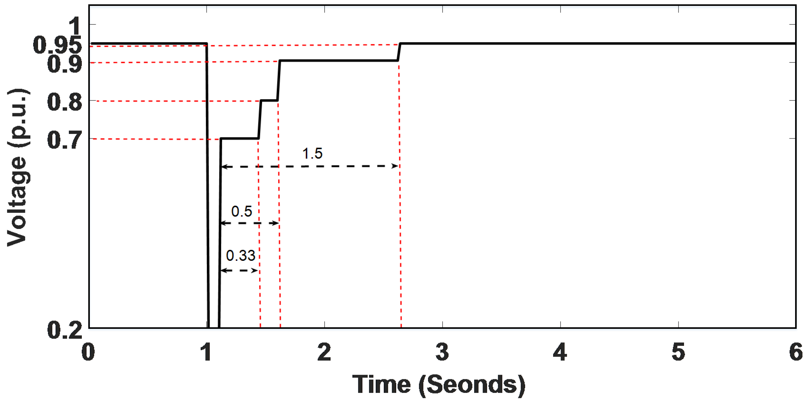
Figure 1. Transient voltage recovery criterion for transmission system [45].
Electronics 15 01377 g001
Figure 2. Architectural overview of cloud–edge collaborative framework.
Electronics 15 01377 g002
Figure 3. The IEEE 300-bus test system [52].
Electronics 15 01377 g003
Figure 4. The learning curve of the Cloud–Edge DRL method.
Electronics 15 01377 g004
Figure 5. Reward difference between cloud–edge collaborative emergency voltage control and centralized emergency voltage control.
Electronics 15 01377 g005
Figure 6. Reward difference between cloud–edge collaborative emergency voltage control and fully-decentralized emergency voltage control.
Electronics 15 01377 g006
Figure 7. Testing results with different methods (a) Performance of the centralized DRL method with fault at bus 163, with fault duration of 0.1 s. (b) Performance of the cloud–edge DRL method with fault at bus 163, with fault duration of 0.1 s. The colored solid lines in the left sub-figures represent the voltage magnitude of the buses in the system while the dotted black line represents the voltage recovery criterion; the colored solid lines in the right sub-figures represent the remaining load fraction of loads in the system.
Electronics 15 01377 g007
Figure 8. Testing results with different methods (a) Performance of the centralized DRL method with fault at bus 258, with fault duration of 0.1 s. (b) Performance of the cloud–edge DRL method with fault at bus 258, with fault duration of 0.1 s. The colored solid lines in the left sub-figures represent the voltage magnitude of the buses in the system while the dotted black line represents the voltage recovery criterion; the colored solid lines in the right sub-figures represent the remaining load fraction of loads in the system.
Electronics 15 01377 g008
Figure 9. Testing results with different methods (a) Performance of the decentralized DRL method with fault at bus 52, with fault duration of 0.1 s. (b) Performance of the cloud–edge DRL method with fault at bus 52, with fault duration of 0.1 s. The colored solid lines in the left sub-figures represent the voltage magnitude of the buses in the system while the dotted black line represents the voltage recovery criterion; the colored solid lines in the right sub-figures represent the remaining load fraction of loads in the system.
Electronics 15 01377 g009
Figure 10. Testing results with different methods (a) Performance of the decentralized DRL method with fault at bus 85, with fault duration of 0.1 s. (b) Performance of the cloud–edge DRL method with fault at bus 85, with fault duration of 0.1 s. The colored solid lines in the left sub-figures represent the voltage magnitude of the buses in the system while the dotted black line represents the voltage recovery criterion; the colored solid lines in the right sub-figures represent the remaining load fraction of loads in the system.
Electronics 15 01377 g010
Table 1. Parameters used in Cloud–Edge Collaborative DRL.
ParametersArea 1Area 2Area 3Coordinator
Policy network size (hidden layers)[16, 16][16, 16][16, 16][16, 16]
Observation space dimension17211530
Action space dimension1518133
Training fault scenarios89711
Number of directions18181824
Top directions88810
Maximum iterations500500500500
Step size1111
Std. dev. of exploration noise2222
Decay rate0.9960.9960.9960.996
Table 2. Comparison of training times for the full-scale centralized and Cloud–Edge approaches.
Centralized full-scale training96.37 h
Cloud–Edge Collaborative training9.59 h
(≈90% saving)
Table 3. Average Inference Time per Control Cycle.
ComponentNetwork SizeAvg. Inference Time (ms)
Edge Agent (Area 1)[16, 16] LSTM + FC11.1
Edge Agent (Area 2)[16, 16] LSTM + FC11.5
Edge Agent (Area 3)[16, 16] LSTM + FC10.9
Cloud Coordinator[16, 16] LSTM + FC12.1
Table 4. Communication Overhead per Control Cycle.
DirectionData ContentPayload SizeEst. Latency
Cloud → EdgeBoolean activation signals ( N = 3 )3 bits< 0.01  ms
Edge → CloudLocal state observation1 KB (per agent)< 0.1  ms
Disclaimer/Publisher’s Note: The statements, opinions and data contained in all publications are solely those of the individual author(s) and contributor(s) and not of MDPI and/or the editor(s). MDPI and/or the editor(s) disclaim responsibility for any injury to people or property resulting from any ideas, methods, instructions or products referred to in the content.