Recurrent Neural Networks with Attention for Indoor Localization in 5G: Evaluation on the xG-Loc Dataset

Abstract

Accurate indoor localization in 5G remains challenging due to multipath propagation, signal blockage, and limited bandwidth in frequency range 1 (FR1). This study evaluates attention-based recurrent neural networks for two-dimensional user equipment (UE) localization using only positioning reference signal (PRS) magnitude data. We compare five models on the xG-Loc dataset (InF-DH scenario at 3.5 GHz, 5 MHz bandwidth): a simple GRU (M1), a deeper GRU with dropout (M2), a GRU optimized via Optuna (M3), a stacked GRU with multi-head attention (M4), and a bidirectional GRU with attention (M5). Model performance is quantified using the area above the cumulative distribution function (CDF) curve (AAC) metric, where lower values indicate better localization accuracy. Attention-based models significantly outperform baselines, and M4 achieves the lowest AAC of 6.71 (17% reduction versus M1’s 8.09), while M5 attains an AAC of 6.90. Statistical analysis confirms that M4 and M5 significantly outperform M3 (ANOVA, p < 0.000001). Optimal performance emerges with moderate numbers of time steps (TS ≈ 500 to 2500), with performance plateauing and degrading at higher values. These findings demonstrate that attention mechanisms substantially enhance 5G indoor localization accuracy using only PRS magnitudes, and that automated hyperparameter optimization improves model robustness.

1. Introduction

Accurate indoor localization is a cornerstone for Industry 4.0, supporting digital twins, resource visibility, and closed-loop optimization, yet performance degrades under multipath, non-line-of-sight (NLOS) blockage, and electromagnetic interference characteristic of factories and warehouses [1]. Technology trade-offs persist, and typical accuracies cluster around decimeter-level for ultra-wideband and meter-level for bluetooth low energy (BLE)/Wi-Fi, with markedly different energy and infrastructure costs [1]. Even among grid-based received signal strength (RSS) methods, robustness hinges on how signals are modeled. Weighted centroid often surpasses trilateration when RSS-to-distance conversion is unreliable, suggesting advantages in learning directly from raw magnitude patterns rather than enforcing brittle propagation models [2].

5G NR provides dedicated positioning signals and timing that, under favorable conditions, enable high accuracy, but results remain sensitive to bandwidth, geometry, synchronization, and channel conditions [3,4]. Over-the-air testbeds with downlink positioning reference signal (PRS) show that larger bandwidths, favorable geometric dilution of precision, and judicious signal processing markedly tighten error distributions, whereas NLOS and small TOA biases can substantially degrade performance. For example, oversampling the channel impulse response (CIR) via zero-padding reduces the 80th-percentile error to about 0.7 m outdoors, highlighting how delay resolution governs accuracy [5]. Other studies combining GNSS pseudoranges with hypothesized 5G ToA/TDoA measurements can improve positioning geometry in urban areas [6]. On commercial FR1 deployments that expose only broadcast synchronization signals, base-station clock offsets and drifts dominate error. After bias compensation and Extended Kalman Filter (EKF) tracking, urban trials still yield multi-meter MAE (≈8–11 m), underlining the need for positioning-grade waveforms and robust inference [7]. Simulation studies further indicate complementary roles for downlink PRS and uplink sounding reference signals (SRS). PRS is preferable in LOS, whereas SRS better tolerates NLOS. Denser tone patterns (smaller combs) consistently reduce ranging error by improving TOA resolution [8]. Dense deployments and 5G large bandwidth make ToA-based ranging feasible, but high accuracy depends on tight synchronization and bias/latency compensation. Early datasets show ToA errors increase indoors and under multipath/NLOS because correlation peaks become distorted [9].

The emergence of 3GPP-compliant datasets offers a rigorous basis to quantify these effects. The xG-Loc dataset spans FR1/FR2, multiple indoor/outdoor deployments, and includes PRS/SRS waveforms, soft-information analytics, and Blockage Intelligence (BI), enabling controlled comparisons across bandwidths and scenarios [10]. In the InF-DH deployment—an indoor factory with heavy multipath and NLOS—soft information-based benchmarks reveal pronounced bandwidth dependence. Percentiles around 1 m (P60) and 2 m (P90) are feasible only when B ≥ 100 MHz, whereas narrowband FR1 (e.g., 5 MHz) is insufficient for comparable ranging-driven accuracy [10]. BI quality is high (ROC-AUC near 0.9), facilitating studies of channel-condition awareness under standardized settings [10].

Beyond waveform design, resource-aware sensing can preserve accuracy while reducing overhead. Using xG-Loc, a learned node activation policy consistently outperforms random selection, preferentially choosing LOS links and limiting the number of active gNBs with controlled performance loss at high percentiles. For example, in IOO and InF-SH, reducing to 4–6 active nodes increases P90 errors modestly relative to using all nodes, while greatly shrinking the combinatorial search for optimal subsets [11]. These results emphasize the value of topology intelligence and selective aggregation, particularly when interference and scheduling budgets constrain the number of usable links.

Data curation critically shapes downstream learning. In ultra-wideband indoor sensing—an adjacent setting facing similar multipath and label-noise issues—principled dataset correction combined with residual architectures lifts LOS/NLOS classification from 80% to above 94%, with measurable gains in feature separability after filtering non-informative CIR regions [12].

Fingerprint-based methods can achieve strong accuracy even with minimal infrastructure. In 5G NR indoor localization, Kalman filtering suppresses received signal strength (RSS) noise while Universal Kriging interpolates sparse reference points. Filtering alone reduces signal variance and improves same-room accuracy by 31%. With interpolation, mean errors approach 1.2 m, and at least 80% of cases remain within 1.6 m, demonstrating sub-2 m reliability from a single small cell [13]. More broadly, bypassing explicit RSS-to-distance conversion enhances robustness under noise [2], motivating sequence models that directly process concatenated PRS magnitude traces across links. The other approach uses an improved ResNet-18 model to estimate user position optimized via an improved genetic algorithm and a Kalman filter [14].

Attention mechanisms and recurrent modeling increasingly improve localization by selectively emphasizing informative features and stabilizing learning under interference. Attention-augmented residual networks operating on time-domain channel features reduce RMSE by up to roughly 50%, considering the 10% injected noise scenario, while maintaining fast inference, indicating that attention pragmatically reweights salient temporal–spatial structure [15]. Robustness further improves with adaptive inference, and treating gNBs as pseudo-satellites and adopting adaptive variational Bayesian filtering yields decimeter-level UAV positioning under interference by handling non-Gaussian disturbances [16]. Meanwhile, learning-aided EKF fusion across heterogeneous 5G cues markedly lowers error compared to any single measurement, underscoring the role of data-driven filters in multipath-rich regimes [17]. Together, this literature converges on attention and temporal aggregation as key levers for resilience when bandwidth and LOS availability are limited.

Building on these insights, the present work targets the xG-Loc InF-DH scenario at 3.5 GHz with 5 MHz bandwidth, where standardized benchmarks show narrowband insufficiency for ranging-based methods [10] and where NLOS is prevalent [11]. The approach intentionally leverages only coherently accumulated PRS magnitudes concatenated across gNBs—eschewing explicit distance or angle estimation to avoid model mismatch—and standardizes features before reshaping to sequence form. This design aligns with evidence favoring magnitude-only learning in noisy environments [2,13] and with demonstrations that attention improves time-domain localization robustness [15].

The study complements recent evidence that resource-aware node selection, synchronization management, adaptive filtering, and attention-driven feature reweighting jointly shape 5G localization accuracy [7,11,15,16]. By demonstrating consistent gains from attention on PRS-magnitude sequences in a standardized, bandwidth-limited InF-DH setting, it is shown that sequence-level learning can extract latent structure otherwise lost to narrowband ranging, offering a practical pathway toward robust indoor localization using signals and measurements already provisioned in 3GPP-compliant datasets.

Contributions: This work provides a controlled study of attention-enhanced GRU architectures for 2D indoor localization on the 3GPP-compliant xG-Loc dataset, focusing on the challenging InF-DH setting at 3.5 GHz with 5 MHz bandwidth. The study intentionally uses only PRS magnitudes (in dB) as inputs to evaluate a minimal fingerprint representation in a narrowband regime, unlike approaches that rely on wideband delay resolution or explicit ranging/angle estimation. The analysis compares five GRU-based models (with/without Optuna tuning, attention, and bidirectionality), quantifies performance using the full error distribution (CDF/AAC) alongside standard metrics, and examines the accuracy–efficiency trade-off as the number of PRS samples (TS) increases.

2. Materials and Methods

2.1. Data Processing

This study employs the InF-DH scenario from the xG-Loc dataset [10], configured at 3.5 GHz with 5 MHz bandwidth. This section summarizes the processing steps applied to the data belonging to this scenario. Section 3 provides a detailed description of its data structure. For each of the 100 runs and 10 user equipments (UEs) per run, the per-UE folder structure is traversed to parse (i) JSON metadata files containing ground-truth 2D positions, and (ii) ZIP archives containing coherently accumulated complex baseband samples of the received positioning reference signal (PRS) per base station (gNB). The JSON files are read to extract Cartesian coordinates [x, y], which are stored in a master table indexed by RUN and UE identifiers.

For model training on large matrices, a two-stage table construction is adopted. First, all per-UE PRS complex series are horizontally concatenated across gNBs and vertically organized across UEs to form tall, wide data frames keyed by standardized column names encoding RUN, UE, and gNB identifiers. Second, to bound memory use during experimentation, a subset is selected comprising all RUNs and a truncated number of PRS time steps (TS) concatenated into the feature dimension. Within this subset, complex samples are transformed into scalar features by computing the magnitude and then converting to decibels. This produces real-valued feature matrices for PRS of shape [N_UE, N_features], where N_features = (number of gNB links) × (number of retained TS). In the main configuration, PRS magnitudes (in dB) are used as inputs.

The xG-Loc PRS observations are available as coherently accumulated complex baseband samples, i.e., both magnitude and phase are present in the raw IQ data. In this study, we intentionally retain only the magnitude (converted to dB) to evaluate a minimal-input setting that is typically more robust to residual phase impairments (e.g., phase noise and carrier/sampling offsets) and more representative of scenarios where only power-like measurements are accessible. We discuss in Section 5 (Limitations and Future Work) how phase- or SRS-based features could further improve performance under multipath.

Target labels are defined as the 2D ground-truth coordinates [x, y] of each UE, extracted from the INFO files and aligned to the corresponding PRS columns by a consistent RUN_UE key. Prior to learning, features are standardized using z-score normalization. The StandardScaler is fitted on the training split and applied to validation and test splits to prevent leakage. The standardized feature matrices are then formatted to be compatible with the GRU architecture while focusing the model on spatial signal structure rather than temporal dynamics. Data are then partitioned into training, validation, and test sets (70/15/15) using stratified randomness via fixed seeds to ensure reproducibility.

2.2. Models & Techniques

2.2.1. Gated Recurrent Unit (GRU)

The Gated Recurrent Unit (GRU) [18,19] is a gated recurrent neural network (RNN) cell that simplifies the LSTM architecture by merging the cell state and hidden state into a single representation.

The dynamics of a GRU cell are governed by the following recurrence relation:

$$h_t=\mathrm{GRU}(x_t,h_{t-1}),$$

(1)

where $x_t$ denotes the input at time step t, and $h_{t-1}$ is the previous hidden state. The internal gating mechanisms are defined as follows:

• Reset Gate ($r_t$): Regulates how much of the previous hidden state contributes to the candidate activation:

  $$r_t=\sigma \left(W_r{x}_t+U_r{h}_{t-1}+b_r\right).$$

  (2)
• Update Gate ($z_t$): Controls the balance between retaining past information and incorporating new content:

  $$z_t=\sigma \left(W_z{x}_t+U_z{h}_{t-1}+b_z\right).$$

  (3)

The candidate hidden state ${\tilde{h}}_t$ and the final output state $h_t$ are then computed:

$${\tilde{h}}_t=tanh\left(W_h{x}_t+U_h\left(r_t\odot h_{t-1}\right)+b_h\right)$$

(4)

$$h_t=z_t\odot h_{t-1}+\left(1-z_t\right)\odot {\tilde{h}}_t$$

(5)

where ⊙ denotes element-wise multiplication, and $\sigma (·)$ represents the logistic sigmoid function.

Intuitively, when $r_t\approx 0$, the influence of the previous state is suppressed, allowing ${\tilde{h}}_t$ to depend primarily on the current input $x_t$. Conversely, when $z_t\approx 1$, the hidden state is preserved across time steps. This mechanism provides near-identity paths for gradient flow, effectively mitigating the vanishing gradient problem. Compared to LSTMs, GRUs achieve comparable performance in modeling long-term dependencies with reduced computational complexity and fewer parameters.

2.2.2. Bidirectional GRU (BiGRU)

A Bidirectional GRU (BiGRU) extends the architecture introduced by Schuster and Paliwal [20]. It enables the model to process sequences in both forward and backward temporal directions, exploiting past and future context simultaneously.

Given an input sequence ${\left\{x_t\right\}}_{t=1}^T$, the hidden states are computed independently:

$$\begin{array}{cc}\hfill h_t^{\mathrm{fw}}& ={\mathrm{GRU}}_{\mathrm{fw}}\left(x_t,h_{t-1}^{\mathrm{fw}}\right)\hfill \end{array}$$

(6)

$$\begin{array}{cc}\hfill h_t^{\mathrm{bw}}& ={\mathrm{GRU}}_{\mathrm{bw}}\left(x_t,h_{t+1}^{\mathrm{bw}}\right).\hfill \end{array}$$

(7)

The bidirectional representation is obtained by concatenating these states, which is then mapped to the output $y_t$:

$$h_t=\left[h_t^{\mathrm{fw}};h_t^{\mathrm{bw}}\right],y_t=f\left(W{h}_t+b\right)$$

(8)

where $f(·)$ is the task-specific activation function.

Training is performed via backpropagation through time (BPTT). Boundary conditions are handled by initializing unknown hidden states (e.g., $h_0^{\mathrm{fw}}$ and $h_{T+1}^{\mathrm{bw}}$) to constant values. Compared to a unidirectional GRU, the BiGRU enhances long-range dependency modeling by accessing future context. This typically results in improved performance at the cost of doubling computational and memory requirements, making it more suitable for non-causal or offline applications.

2.2.3. Dropout

Dropout is a regularization technique that prevents co-adaptation and reduces overfitting by randomly deactivating units during training [21].

During training, a binary mask r is sampled from a Bernoulli distribution:

$$r\sim \mathrm{Bernoulli}\left(p\right).$$

(9)

In the inverted dropout formulation, activations h are rescaled during training to maintain consistent expectations at inference:

$$h^{\ast }={\displaystyle \frac{1}{p}}\left(r\odot h\right).$$

(10)

Dropout approximates the average prediction of an implicit ensemble of $2^n$ thinned networks. In practice, retention probabilities are typically set to $p\approx 0.5$ for hidden layers and $p\approx 0.8$–$0.9$ for input layers. Combining dropout with max-norm constraints and learning rate decay further stabilizes optimization, consistently reducing generalization error across vision, speech, and natural language processing tasks.

2.2.4. Attention Mechanism

Attention mechanisms [19,22] compute relevance-weighted combinations of information, allowing a model to focus on the most informative elements of a sequence.

The core operation is the scaled dot-product attention:

$$\mathrm{Attention}(Q,K,V)=\mathrm{softmax}\left({\displaystyle \frac{Q{K}^{\top }}{\sqrt{d_k}}}\right)V$$

(11)

where Q, K, and V are the query, key, and value matrices, and $d_k$ is the dimensionality of the keys. The scaling factor $\sqrt{d_k}$ ensures numerical stability.

To enhance representational capacity, multi-head attention projects the input into h subspaces:

$$\mathrm{MultiHead}(Q,K,V)=\mathrm{Concat}\left({\mathrm{head}}_1,\dots ,{\mathrm{head}}_h\right)W^O$$

(12)

$${\mathrm{head}}_i=\mathrm{Attention}\left(Q{W}_i^Q,K{W}_i^K,V{W}_i^V\right).$$

(13)

Standard configurations include:

• Encoder self-attention: All positions attend to each other.
• Masked self-attention: Prevents attending to future positions (causal).
• Encoder-decoder attention: Queries attend to encoder representations.

This design achieves a constant path length $O\left(1\right)$ between sequence positions and offers high parallelism compared to recurrent architectures. In applied domains like 5G localization, attention highlights salient patterns (e.g., traffic bursts) while suppressing noise, and can be integrated into GRU-based models or used in fully attention-based encoders.

2.3. Hyperparameter Optimization with Optuna

Optuna [23] is a hyperparameter optimization framework built around a define-by-run API, enabling users to construct complex, conditional search spaces directly in Python (version 3.12.12) using loops, conditionals, and modular helper functions. This approach keeps optimization code concise, readable, and reusable while enabling easy deployment via FixedTrialto reproduce chosen settings.

The framework supports both independent samplers, such as Tree-structured Parzen Estimator (TPE), and relational samplers, such as Covariance Matrix Adaptation Evolution Strategy (CMA-ES) and Gaussian Process-based Bayesian Optimization (GP-BO). Optuna automatically infers which parameters co-occur so that relational samplers are applied only when informative; mixing TPE for early steps with CMA-ES later provides a strong default strategy.

To conserve computational resources, Optuna (version 4.7) provides first-class pruning through an asynchronous variant of Successive Halving (ASHA) via report() and should_prune(). This mechanism safely terminates underperforming trials early and proves especially effective in distributed settings. The system runs with in-memory storage for notebooks or with SQLite and relational databases for multi-process studies, achieving near-linear speedups with additional workers.

Search-space bounds (

Table 1. Summary of the hyperparameters search spaces for models M3, M4, and M5.

Hyperparameter	M3	M4	M5
n_layers	[1, 4]	[1, 4]	[1, 4]
units_first	[32, 256]	[32, 256]	[32, 256]
dropout_rate	[0.1, 0.5]	[0.1, 0.5]	[0.1, 0.5]
learning_rate	[10−5, 10−2 (log)]	[10−5, 10−2 (log)]	[10−5, 10−2 (log)]
batch_size	{16, 32, 64, 128}	{16, 32, 64, 128}	{16, 32, 64, 128}
num_heads	–	[1, 8]	[1, 8]

) were selected to span edge-feasible model sizes while keeping the number of trials computationally tractable. To reduce overfitting during optimization, early stopping on validation loss and dropout after recurrent layers were applied. Hyperparameters were selected using validation performance only, and the held-out test set was evaluated once per finalized configuration. In Table 1, brackets […] denote continuous/integer ranges, braces {…} denote categorical choices, and (log) indicates log-uniform sampling.

2.4. Model Building

Five distinct deep learning architectures are employed for indoor UE localization, progressively increasing in complexity. Model M1 implements a baseline architecture consisting of a single GRU layer with 50 units and ReLU activation, followed by a dense output layer with 2 units corresponding to the predicted x and y coordinates. The model is compiled with the Adam optimizer and mean absolute error loss function, trained for a maximum of 500 epochs with a batch size of 32 and early stopping patience of 20 epochs.

Model M2 extends this baseline by implementing a deeper architecture with three stacked GRU layers, each containing 128 units with ReLU activation and return sequences enabled for the first two layers. Dropout regularization with a rate of 0.2 is applied after each GRU layer to mitigate overfitting, maintaining the same training configuration as M1 with 500 maximum epochs, batch size of 32, and patience of 20.

The Optuna framework optimized hyperparameters for models M3, M4, and M5 through 50 Bayesian optimization trials each, with validation loss serving as the objective function. Table 1 summarizes the search spaces explored for each architecture. Model M3 employs a sequential GRU architecture with variable depth and width. Intermediate GRU layers receive unit configurations sampled from the search space, with dropout applied after each recurrent layer. The architecture terminates in a dense output layer for regression.

Model M4 extends the M3 foundation by incorporating self-attention mechanisms. The architecture stacks GRU layers with return sequences enabled, then applies a Keras MultiHeadAttention layer in self-attention mode (MultiHeadAttention (num_heads = num_heads, key_dim = units_first) (x, x)), where queries, keys, and values all derive from the recurrent output sequence x. An additive residual connection sums the attention output with the original sequence representation (attn_out + x), followed by post-normalization via LayerNormalization(epsilon = $1\times {10}^{-6}$). Global average pooling aggregates the temporal dimension before the final two-unit dense layer.

Model M5 maintains the M4 architecture with one critical modification. Bidirectional GRU layers replace all standard GRU layers, doubling the sequence channel size and enabling bidirectional temporal processing. The attention module operates as MultiHeadAttention (num_heads = num_heads, key_dim = key_dim) (x, x), where key_dim remains constrained to the BiGRU output width. The architecture optionally applies global average or max pooling for temporal aggregation and incorporates L2 regularization on the output dense layer. All three models employed early stopping with 10-epoch patience on validation loss, training for a maximum of 100 epochs during hyperparameter optimization.

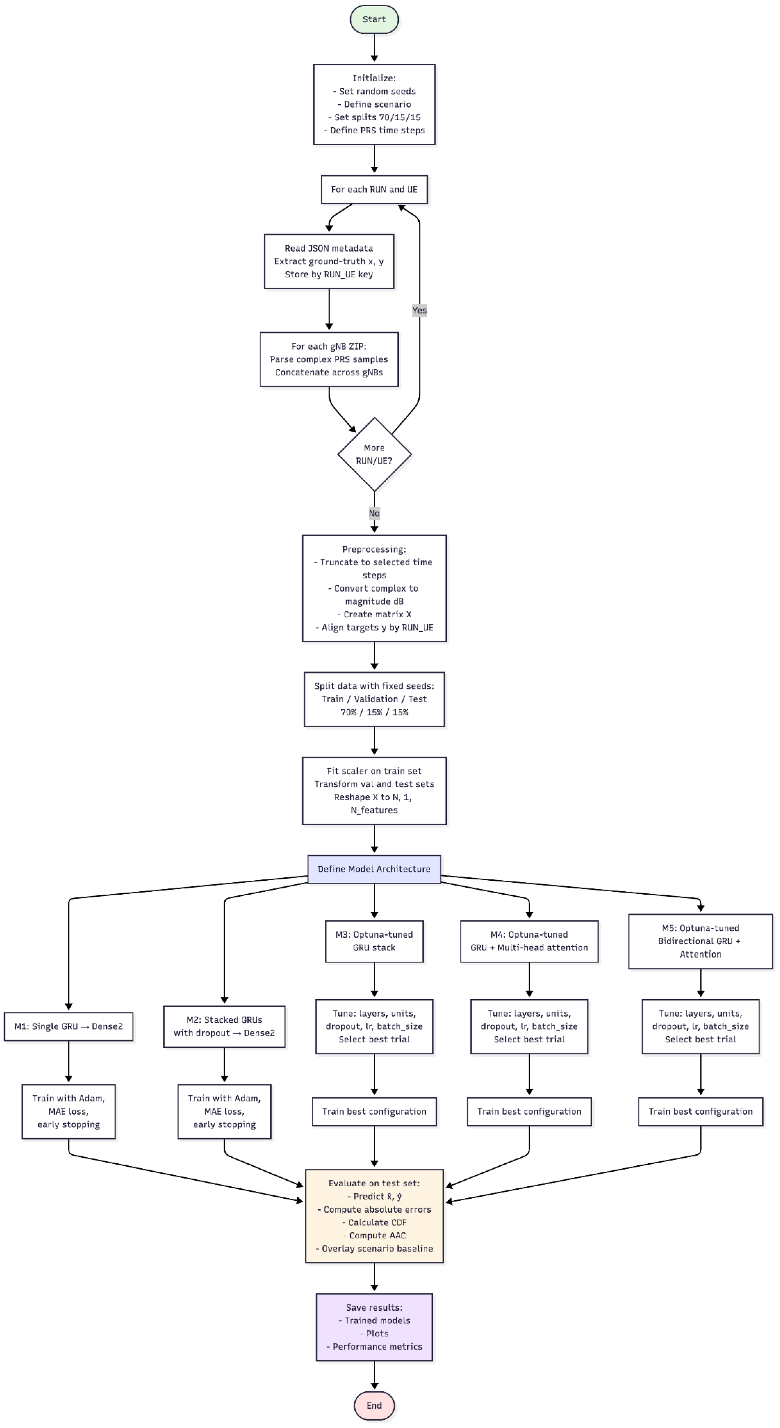
Figure 1 illustrates the end-to-end pipeline used for training and evaluating the GRU-based localization models using positioning reference signal (PRS) data. The pipeline begins with data preparation, in which complex PRS samples are extracted from gNB files, concatenated across base stations, converted to decibel magnitude, and aligned with ground-truth coordinates from JSON metadata. The dataset is then split into training, validation, and test sets using a 70/15/15 ratio with fixed random seeds to ensure reproducibility. Following standardization and reshaping for GRU input compatibility, the five model architectures are trained using the Adam optimizer with MAE loss and early stopping. For the optimized models, hyperparameter tuning explores architectural depth, hidden unit counts, dropout rates, learning rates, and batch sizes. Final evaluation on the test set includes computation of localization errors, generation of cumulative distribution functions (CDFs), calculation of area-above-CDF metrics, and comparison against published baselines, with all intermediate results and configurations saved to ensure full reproducibility.

2.5. Dataset

This study employs the xG-Loc dataset [10], a public, 3GPP-compliant corpus for localization research generated using the QuaDRiGa channel model with spatial consistency across channels and scenarios. The analysis focuses on the Indoor Factory–Dense High (InF-DH) scenario operating at 3.5 GHz with a bandwidth of 5 MHz, numerology $\mu =0$, and $N_{\mathrm{RB}}=24$. The simulated environment spans 120 m × 60 m and comprises 18 single-sector gNB sites, deployed at a height of 8 m with an inter-site distance of 20 m.

User equipment (UE) locations are generated via drop-based uniform sampling at a height of 1.5 m. UEs are equipped with omnidirectional antennas and transmit at 23 dBm, while gNBs transmit at 24 dBm. The dataset adheres to a spatially consistent channel parameterization, with correlation distances of 10 m for large-scale channel parameters and 1 m for state variations. Scenario generation assumes an effective clutter height of 2 m, a typical clutter size of 2 m, and a clutter density of 40%. For each configuration, $N_{\mathrm{RUN}}=100$ independent runs are provided, each containing $N_{\mathrm{UE}}=10$ UEs, resulting in a total of 1000 UE instances. Each UE instance includes preprocessed received PRS/SRS samples per gNB and an associated metadata JSON file containing ground-truth positions and derived measurements.

The dataset artifacts used in this work include, for each UE, coherently accumulated received reference signal samples (PRS/SRS) from each gNB, the true three-dimensional position $[x,y,z]$, a two-dimensional side-information estimate $[\widehat{x},\widehat{y}]$ derived from round-trip timing (RTT), per-link range proxies $(c·\widehat{T})$ for downlink and uplink, binary link-state indicators, and blockage intelligence probabilities $\psi$ describing the likelihood of obstruction on each link. Additional top-level files provide the corresponding transmitted reference signals and global metadata, including scenario definitions, gNB coordinates, and sampling rates.

For the InF-DH scenario at 3.5 GHz with 5 MHz bandwidth, no angular estimates are available in FR1, constraining the feature set to the provided reference signal observations and link-quality indicators. Across runs and UEs, this structure enables supervised learning with paired inputs (per-link signal observations and auxiliary link metrics) and outputs (UE positions), while preserving physical realism through 3GPP-compliant spatial consistency and site geometry.

To contextualize task difficulty, Conti et al. [10] report horizontal positioning error statistics for soft-information (SI)-based localization relying solely on RTT measurements. Among all evaluated configurations, the InF-DH scenario at 3.5 GHz with 5 MHz bandwidth exhibits the largest error percentiles (

Table 2. Error percentiles in InF-DH scenario at 3.5 GHz with 5 MHz bandwidth [10].

Dataset	10th	20th	30th	40th	50th	60th	70th	80th	90th	95th	99th
infdh_5_3.5	3.95 m	6.05 m	7.97 m	9.82 m	11.50 m	13.48 m	16.05 m	19.53 m	26.72 m	36.72 m	55.65 m

).

These reported values are adopted in this work as a reference baseline for the same configuration. Comparisons are conducted strictly against the corresponding entries in Table 2, ensuring that any observed performance gains are attributable to learning-based inference under identical data, geometry, and bandwidth conditions.

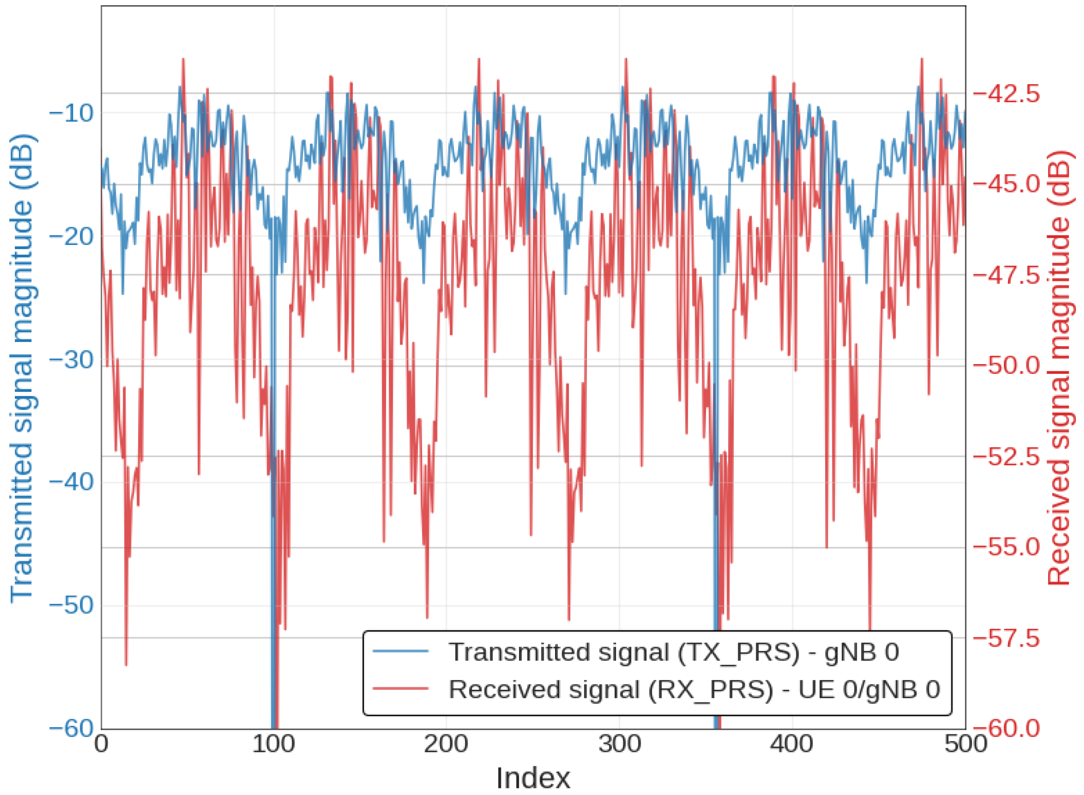
Figure 2 illustrates a representative snapshot of the PRS signals. The blue trace shows the magnitude of the transmitted positioning reference signal (TX_PRS) on a decibel scale as a function of the sample index. The red trace (right-axis scale) depicts the coherently accumulated received PRS magnitude for UE 0 from gNB 0. The received signal envelope follows the PRS structure but is attenuated by approximately 30–40 dB and exhibits fast temporal fluctuations caused by small-scale fading, as well as occasional deep fades. This behavior highlights the signal-to-noise ratio regime and temporal variability characterizing the observations used for learning-based localization.

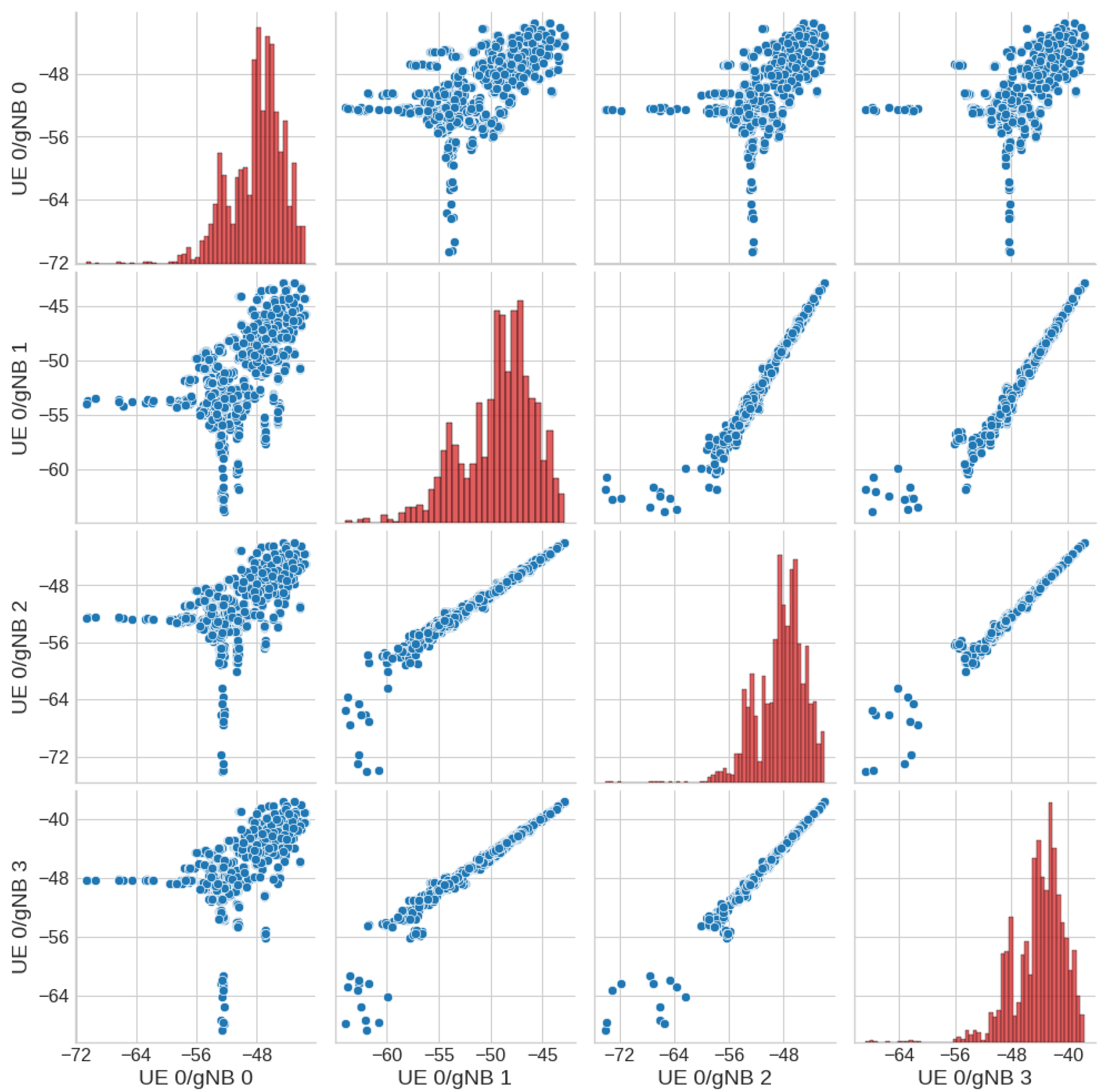
Figure 3 presents a pair plot of the received PRS magnitudes for UE 0 across the first four gNBs in RUN 0. The diagonal panels show marginal histograms for each UE–gNB link, revealing distinct power distributions that reflect differences in path loss and blockage conditions. The off-diagonal panels display scatter plots between pairs of links, several of which exhibit strong positive and near-linear correlations, consistent with shared geometry and correlated slow-fading effects under spatial consistency.

The presence of outliers and clusters at very low received power levels indicates intermittent deep fades or partial blockage events. Overall, the figure demonstrates that while multi-link observations are heterogeneous and heteroscedastic, they are statistically coupled, capturing the structural characteristics of the InF-DH environment in the xG-Loc dataset.

3. Results and Discussion

3.1. Model Convergence and Localization Accuracy

This section presents the comparative evaluation of model performance, focusing on the progressive improvement in prediction quality from the simple model M1 onwards. To quantify performance differences, the area above the CDF curve (AAC) serves as the principal metric, providing a direct measure of how closely prediction errors cluster around smaller magnitudes. This metric enables consistent comparisons across all models.

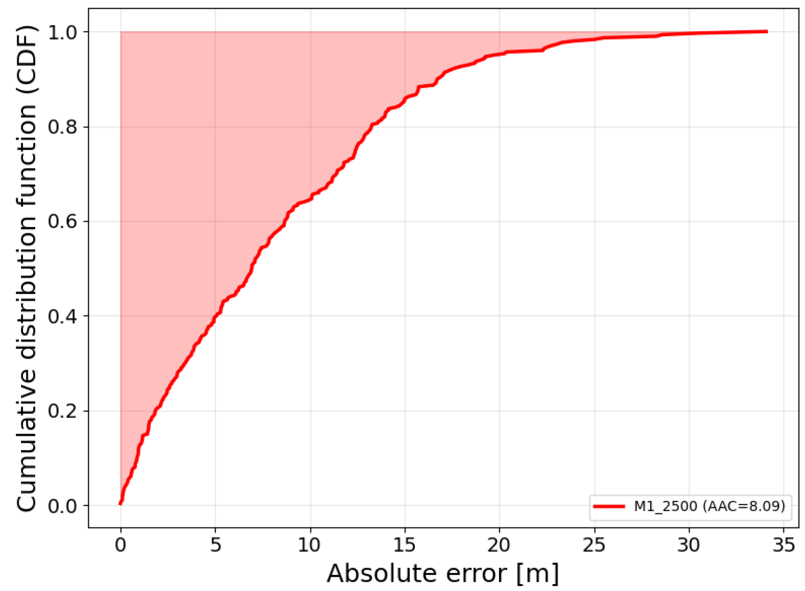
Figure 4 depicts the AAC metric through the cumulative distribution function (CDF) of localization error for model M1 trained using 2500 time steps (TS) as a reference. The light red shading highlights the AAC, defined as the region between the CDF curve and the maximum cumulative probability line at y = 1. This visualization emphasizes the deviation of each model’s error distribution from the ideal case of perfect localization (AAC = 0). Lower AAC values correspond to curves that rise more steeply toward the upper boundary, indicating that errors concentrate at smaller magnitudes and thus reflect superior localization accuracy.

Table 3. Parameters for each of the best models found in this work. M = Model, TS = Time steps.

	GRU		BiGRU		Dense		Dropout		Attention
Model	Layers	Units	Layers	Units	Layers	Units	Layers	Units	Layers	Heads	Optuna	Epochs	TS	AAC
M1	1	50	–	–	1	2	–	–	–	–	No	75	2500	8.09
M2	3	128 × 3	–	–	1	2	3	0.2 × 3	–	–	No	94	500	8.00
M3	4	41, 77, 235, 172	–	–	1	2	4	0.147 × 4	–	–	Yes	158	250	7.46
M4	1	100	–	–	1	2	1	0.468	1	6	Yes	86	750	6.71
M5	–	–	1	34	1	2	1	0.405	1	3	Yes	68	1500	6.90

presents the main results of the training experiments. The simple model, M1, consists of a single GRU layer with 50 units followed by a dense output layer with 2 units. This simple architecture achieves its best results when trained on the first 2500 TS for 75 epochs and provides a lightweight reference point against which more complex models are evaluated. Building on this foundation, model M2 introduces greater depth by stacking three GRU layers of 128 units each, combined with dropout regularization to mitigate overfitting. M2 obtains its best results using 500 TS and explores the benefits of increased representational capacity. Both models obtain an AAC of approximately 8.0, indicating no relevant error reduction at this stage.

To further refine performance, M3 employs four GRU layers with 41, 77, 235, and 172 units and incorporates dropout. Its key distinction lies in the use of Optuna for hyperparameter optimization. This approach allows the model to adapt its configuration more effectively to the data (including the optimal number of GRU layers and units), obtaining its best results using only 250 TS. Model M4 comprises one GRU layer with 100 units, integrates dropout, and importantly introduces a multi-head attention mechanism. This addition enables the model to focus selectively on the most informative features, enhancing its ability to capture complex relationships in the input signals. Like M3, it benefits from Optuna-driven optimization, with best results obtained using 750 TS during training. Overall, M4 achieves the lowest error as measured by AAC (6.71).

Finally, M5 combines a bidirectional GRU with an attention mechanism, allowing it to capture dependencies in both forward and backward directions of the sequence. With 34 units in the BiGRU layer, dropout regularization, and three attention heads, this model represents the most sophisticated configuration in the study. It is also optimized with Optuna and trained for 68 epochs, with best results obtained using 1500 TS. This model corresponds to the second-best configuration, after M4, as evidenced by its AAC (6.90).

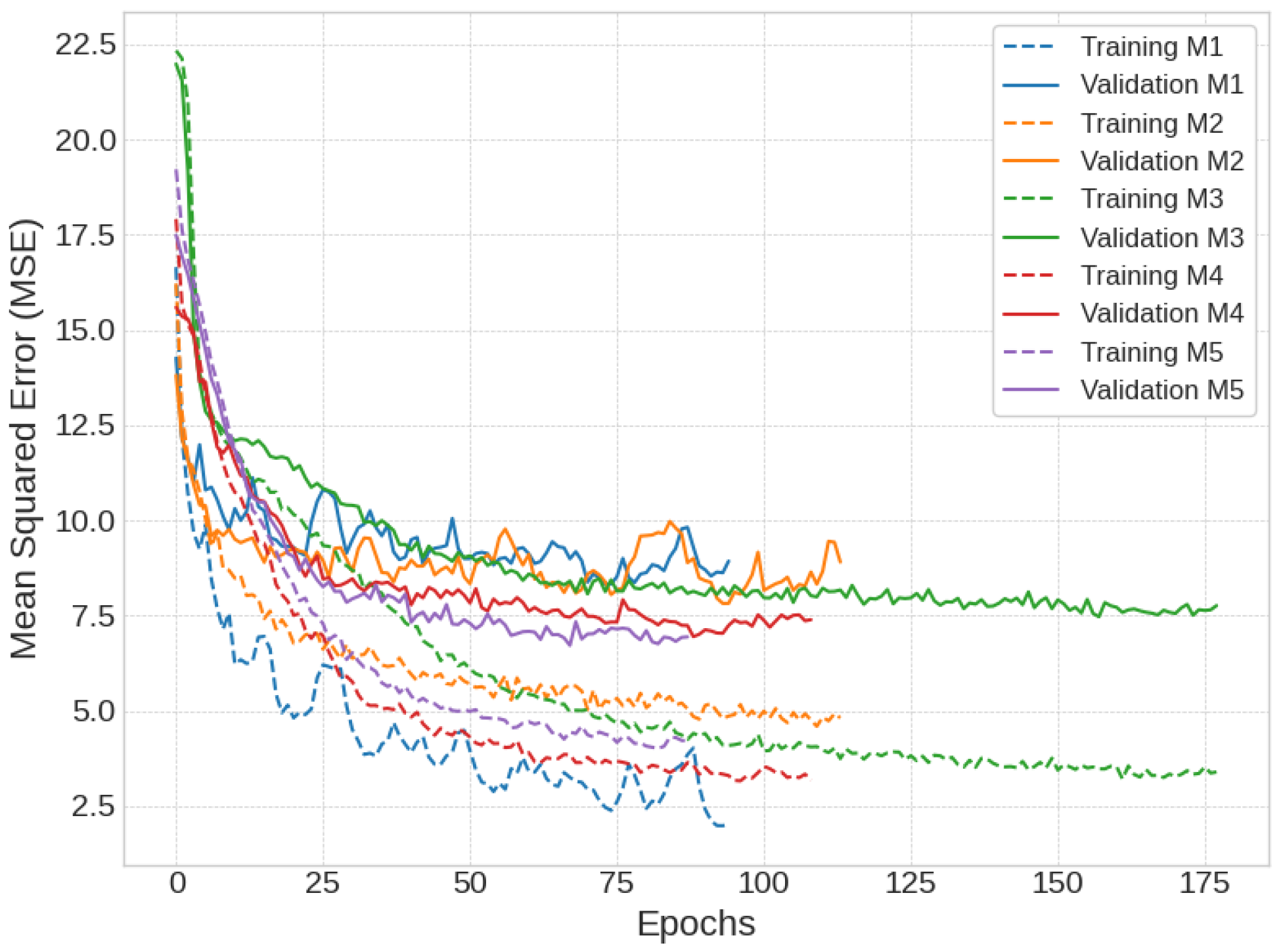
Figure 5 presents the training and validation loss curves obtained for the five models under study. The x-axis shows the full training histories, while the ’Epochs’ column in Table 3 lists the best epoch selected by early stopping. The simple model (M1) exhibits a steep reduction in training loss, yet the validation curve stabilizes at a relatively high level, indicating limited generalization capacity. Both training and validation curves present an appreciable level of fluctuations that suggest the onset of overfitting. When additional GRU layers and dropout are introduced in M2, the training curve descends less steeply, but the validation curve still shows sizable fluctuations. The incorporation of hyperparameter optimization in M3 produces smoother trajectories, with the validation curve converging at a slightly lower value than in the previous models, reflecting improved adaptation to the data.

The effect of attention mechanisms becomes evident in M4, where the validation curve descends smoothly to a level noticeably lower than the previous models. This behavior demonstrates enhanced stability and generalization, consistent with the quantitative improvements reported in Table 3. Finally, M5, which combines bidirectional GRUs with attention, achieves performance comparable to M4. Its validation curve descends to a level similar to M4, with comparable smoothness. The Figure 5 illustrates the progressive improvement in convergence behavior as architectural complexity and optimization strategies are introduced, culminating in the superior performance of the attention-based models improved through Optuna hyperparameter optimization.

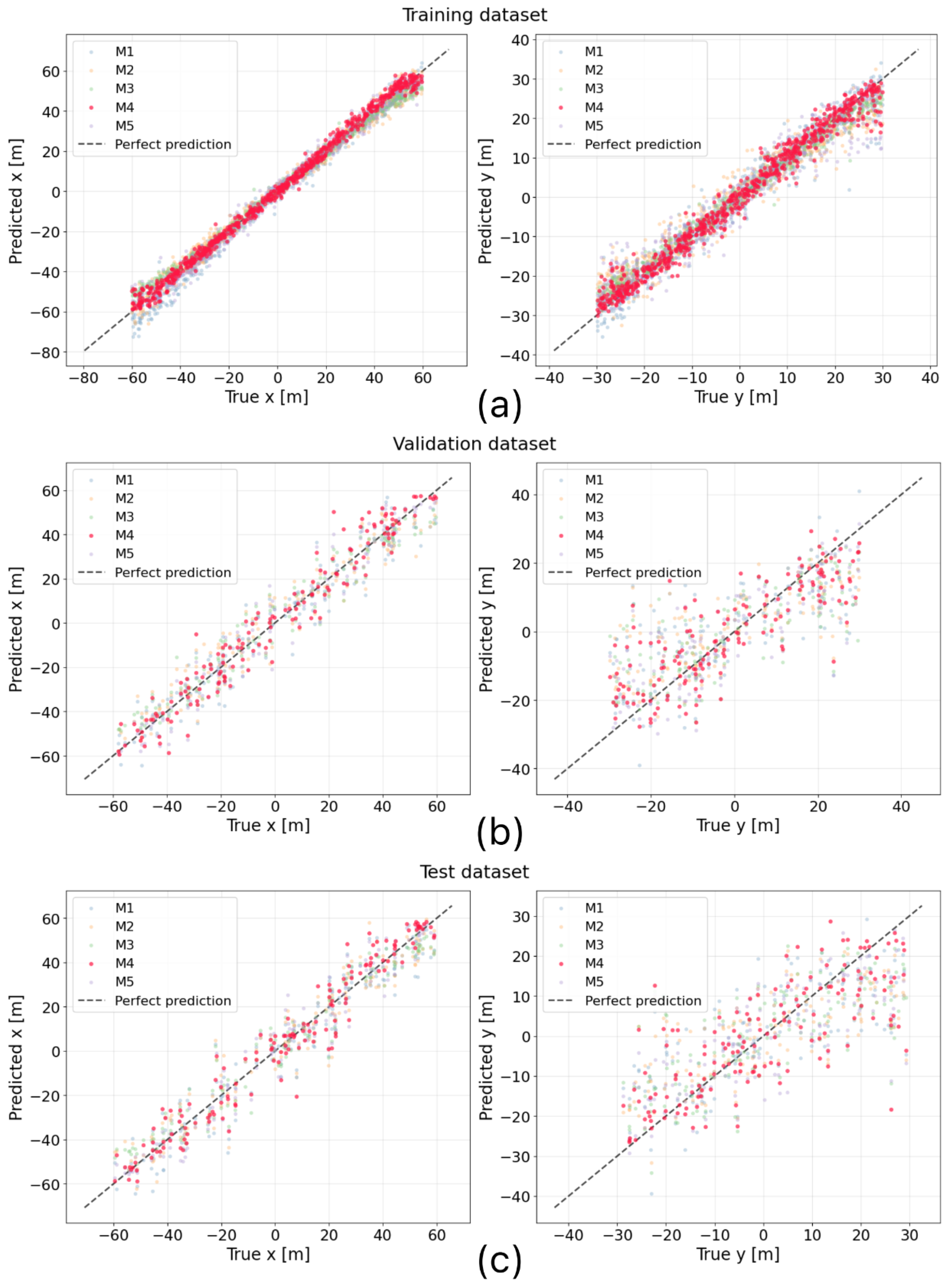
Figure 6 compares true versus predicted x and y coordinates for the five models (M1 to M5) across the three data splits: (a) training, (b) validation, and (c) test. Each panel shows scatter plots of predicted versus true x (left column) and y (right column) values, with the diagonal line indicating perfect prediction. The legend identifies M1 to M5 models, while points from the attention-based model M4 appear highlighted in crimson red to facilitate visual comparison.

In the training set (panel a), all models closely follow the diagonal line of perfect prediction for both x and y coordinates, with the majority of points tightly clustered around it. However, at both extremes, the points begin to scatter more noticeably from the perfect prediction line. The scatter in the y coordinates (right) appears larger than in the x coordinates. This behavior on the training data indicates that even the simpler architectures can fit the observed trajectories when evaluated on seen samples. In the validation set (panel b), small differences among models become apparent. However, this type of plot does not readily reveal the superiority of more precise models such as M4 over the others. Again, the scatter in the y-axis appears more pronounced than in the case of the x coordinate. In the test set (panel c), the trends observed on the validation set persist on the held-out test data. M4 results maintain a slight edge with respect to the others, while again the y-axis shows a larger scatter of points.

Figure 6 visually corroborates that the error in the training dataset remains smaller than in the validation and test datasets and that predicting the y-axis of the location coordinates presents greater difficulty. This difficulty is influenced by the 2D floor-plan geometry (120 m in the x-dimension and 60 m in the y-dimension) and by the gNB layout, which provides denser variation along x than along y in this deployment. Note that the “8 m height” reported for gNBs refers to the z-axis (installation elevation), not to the y-dimension of the floor plan (see Figure 1a in Conti et al. [10]).

Table 4. Summary of the MAE, RMSE and AAC results for the test dataset.

Model	MAE (x)	MAE (y)	RMSE (x)	RMSE (y)	AAC
M1	7.16	9.13	9.20	11.52	8.09
M2	6.77	9.36	8.74	11.73	8.00
M3	6.46	9.27	8.00	11.68	7.46
M4	6.42	7.89	8.00	10.39	6.71
M5	6.74	8.14	9.39	10.74	6.90

presents performance metrics for the five models (M1-M5) on the test dataset. M4 achieves the best overall performance with the lowest MAE values (6.42 for x, 7.89 for y), the best AAC score of 6.71, and shares the lowest RMSE (x) of 8.00 with M3, while also maintaining the lowest RMSE (y) at 10.39. M5 ranks second with strong y-coordinate predictions but weaker x-coordinate accuracy, while M1 shows the poorest performance across all metrics with the highest errors. M2 and M3 demonstrate intermediate performance, with M3 achieving a competitive AAC of 7.46. The results indicate progressive improvement from M1 to M4, with M4 representing the most accurate model for localization tasks.

3.2. Impact of Time Steps on Performance

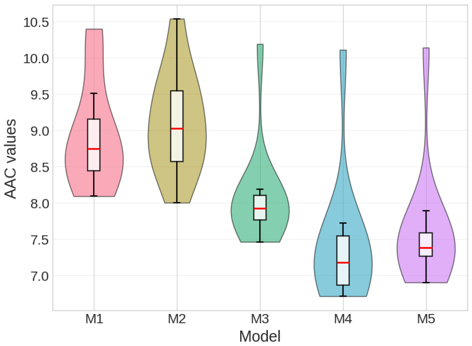
Figure 7 presents the distribution of AAC values for the five competing models (M1 to M5) using violin plots with embedded boxplots, combining density estimation with range visualization. The AAC values on the y-axis correspond to results from training and testing each model with different time step (TS) values, representing the number of data points extracted from the magnitude in decibels of the PRS signal. Each model yields 12 different results, as TS values range from 10 to the maximum possible value in the data (3288). The precise TS values are indicated along the horizontal axis of the figure. The AAC metric quantifies prediction error, where lower values indicate better model performance.

The results reveal distinct performance tiers among the models. M1 and M2 demonstrate the weakest performance, with AAC median values at approximately 8.75 and 9.0, indicating both low accuracy and high variability as shown in the interquartile range (IQR) of the boxplots. M3 shows intermediate performance with a median near 8.0 and reduced distribution spread, reflected in its shorter IQR.

In contrast, M4 and M5 display notably stronger performance, with median AAC values around 7.2 to 7.4 and narrow IQR lengths, particularly for model M5. The elongated violin shapes for these models indicate the presence of outliers corresponding to models trained using only 10 TS, as shown in Figure 7. This figure clarifies not only which models perform best but also whether the performance differences are practically meaningful. The visualization thus provides clear evidence that M4 and M5 represent the most effective modeling approaches, achieving consistently lower error levels with reduced variability.

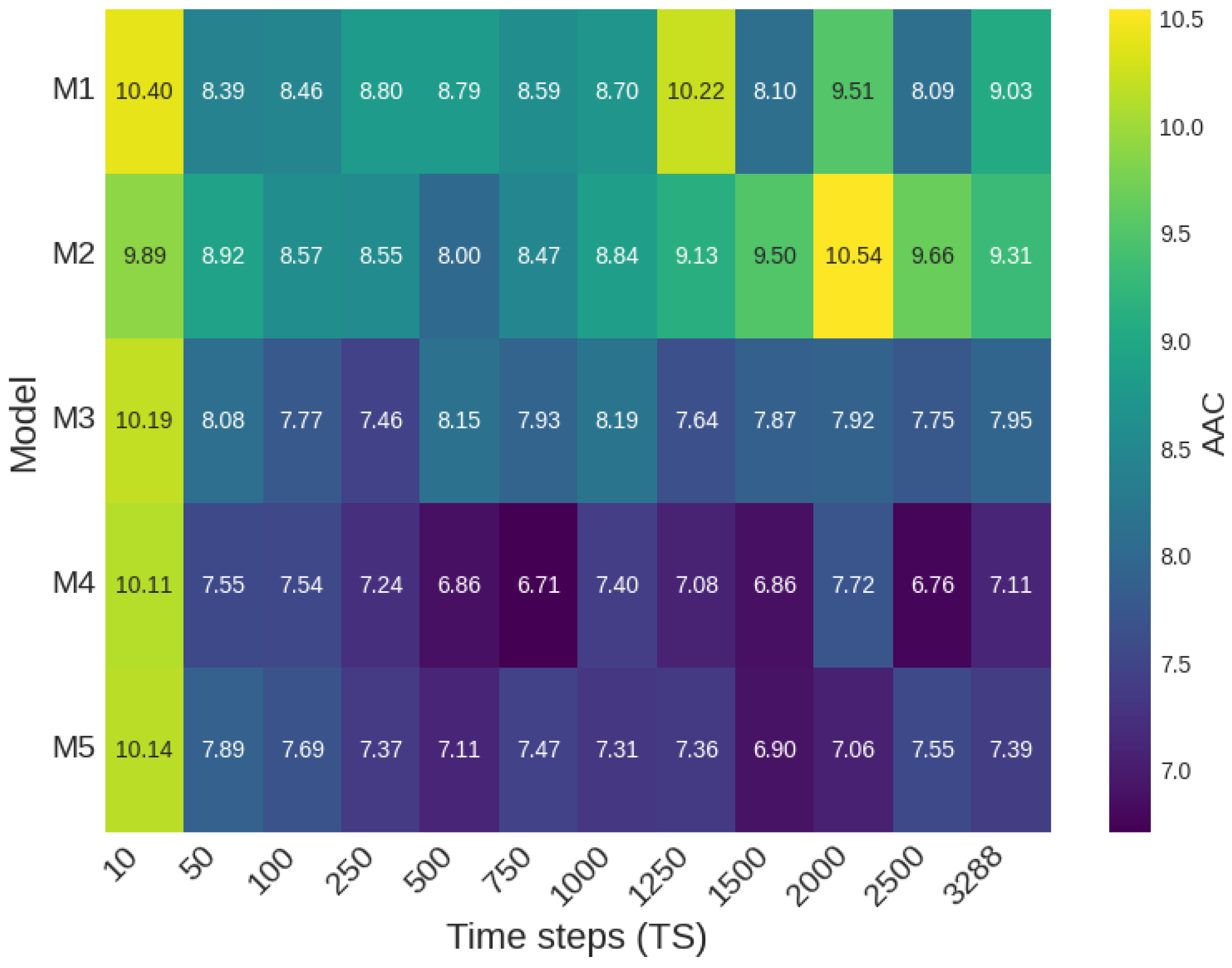
Figure 8 presents a heatmap illustrating the relationship between the number of TS used in training and AAC values across the five model configurations (M1 to M5). The visualization employs a continuous color scale where darker regions indicate lower AAC values and lighter regions correspond to higher AAC values. The horizontal axis represents TS ranging from 10 to 3288, while the vertical axis displays the five model variants.

The heatmap reveals distinct performance patterns as the number of TS increases. Performance variation is nonuniform across configurations, with certain regions exhibiting decreased AAC values, indicating improved accuracy, and others showing relatively elevated values, indicating less favorable outcomes. Models M1 and M2 produce consistently higher AAC values (8.00 to 10.54) across most time step configurations, with M2 showing a notable peak at 2000 TS. In contrast, models M3, M4, and M5 exhibit lower AAC values overall, with M4 and M5 achieving optimal performance (lowest AAC values of 6.71 and 6.90, respectively) within the range of 500 to 2500 TS. Model M4 shows particularly strong performance at 750 and 2500 TS, while M5 maintains relatively stable low values across the 500 to 2000 range. The visualization emphasizes the sensitivity of model performance to input data length and provides a comprehensive overview of how training efficiency and error metrics depend on the volume of temporal samples utilized.

Increasing TS increases the input sequence length and, therefore, the amount of information presented to the model. However, beyond a moderate TS range, additional PRS samples are often highly correlated and can be dominated by fading/noise realizations, while also increasing effective model capacity needs relative to the limited number of trainings UEs (N = 1000). This can lead to diminishing returns and occasional degradation in generalization. From a system perspective, this suggests selecting a moderate TS that balances accuracy against inference cost.

3.3. Robustness Analysis and Computational Efficiency

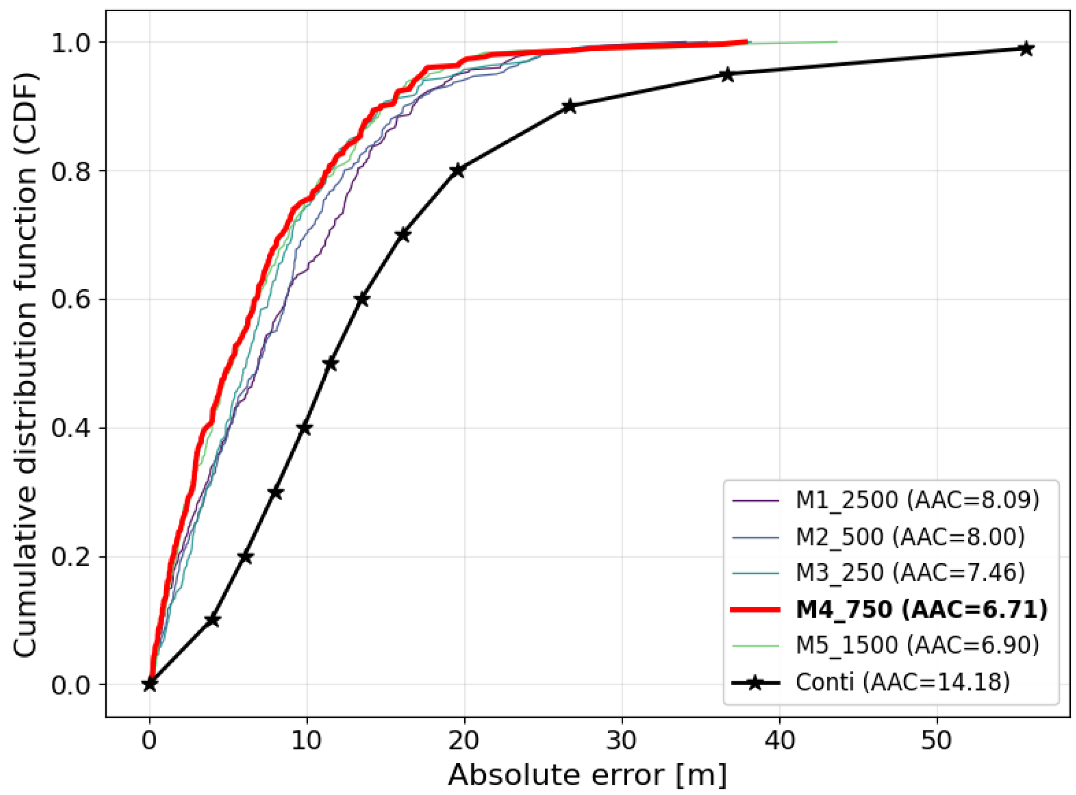
Figure 9 depicts the cumulative distribution functions (CDFs) of localization error for the baseline reference and the five proposed models. The curves allow direct comparison of how frequently smaller errors occur across different architectures. The baseline reference, drawn from Conti et al. [10], shows relatively high error percentiles in the InF DH scenario at 3.5 GHz with a 5 MHz bandwidth configuration: the 50th percentile at 11.50 m, the 90th at 26.72 m, the 95th at 36.72 m, and the 99th at 55.65 m.

Against this benchmark, the trained models progressively shift the CDF curves upward and leftward, indicating improved accuracy. The simplest GRU model (M1) and its deeper variant (M2) achieve noticeable gains, with AAC values near 8.0, meaning that approximately 90% of errors fall below 15 m. Model M3, optimized with Optuna, reduces the AAC to 7.46, concentrating more probability mass at lower distance levels.

The most pronounced improvement is observed with M4, which integrates multi-head attention. Its AAC drops to 6.71, and the CDF shows that a larger proportion of UE location errors concentrates at lower values compared to earlier models. The bidirectional GRU with attention (M5) follows closely, with an AAC of 6.90, also demonstrating a substantial reduction in high percentile errors.

Figure 9 highlights a clear performance hierarchy. While the baseline curve indicates that nearly 90% of cases fall below 26.72 m error, the attention-based models reduce this threshold significantly, concentrating the majority of predictions below the 15 m error level. The numerical shifts in percentiles and AAC values confirm that attention mechanisms yield the most consistent accuracy gains.

To account for the stochastic nature of hyperparameter optimization, models M3, M4, and M5 undergo 10 independent Optuna runs each. Specifically, M3 receives optimization when trained using 250 time steps (TS) of data, M4 using 750 TS, and M5 using 1500 TS, with each configuration explored across 10 separate runs. The results presented in Figure 9 correspond to the best-performing run for each model. A subsequent statistical analysis of the 10 AAC values obtained per model reveals important insights into their comparative performance and variability. Model M3 exhibits a mean AAC of 7.73 with a standard deviation of 0.13, indicating highly consistent performance across runs. Model M4 achieves the lowest mean AAC of 7.03, though with greater variability (standard deviation of 0.27), while M5 shows intermediate performance with a mean of 7.20 and standard deviation of 0.22. One-way ANOVA confirms statistically significant differences among the three models (F = 29.25, p < 0.000001). Post-hoc pairwise comparisons using Bonferroni-corrected t-tests reveal that M4 significantly outperforms M3 (p < 0.000001) and that M5 significantly outperforms M3 (p < 0.000004), while the difference between M4 and M5 remains not statistically significant (p = 0.134). These findings confirm that the multi-head attention mechanism in M4 delivers the most robust accuracy gains, despite introducing additional performance variability across optimization runs.

To strengthen the evaluation, two lightweight learning baselines commonly used in fingerprinting applications, Support Vector Regression (SVR) and a compact Convolutional Neural Network (CNN) were added. These methods offer a fair comparison while maintaining computational feasibility for edge deployment scenarios. The SVR method fits kernel regressors on standardized feature vectors using an RBF kernel with C = 100, gamma = ‘scale’, and epsilon = 0.1. Two separate SVRs, one predicting x coordinates and one predicting y coordinates, were trained, then stacked their outputs to form the final (x,y) prediction. Both methods were evaluated using coordinate-wise RMSE on train/validation/test splits.

The CNN method treats each sample as a 1D signal by reshaping the standardized PRS-derived feature vector to (n_features, 1) and learns location through a regression network. The architecture contains three convolution blocks, Conv1D (64, kernel = 5), Conv1D (128, kernel = 5), Conv1D (64, kernel = 3), each using ReLU activation, BatchNormalization, MaxPooling1D, and Dropout. A Flatten layer connects to Dense(128), Dense(64), and Dense(2) layers that output (x,y) coordinates. The model is trained using the Adam optimizer (learning rate 0.001), with early stopping and best-model checkpointing based on validation loss.

Both baseline learning methods obtain inferior performance compared to the proposed approaches. The SVR baseline achieves RMSE (x) of 9.95, RMSE (y) of 12.38, and AAC of 12.54. The CNN baseline performs similarly with RMSE (x) of 9.21, RMSE (y) of 12.41, and AAC of 13.11. The best model (M4) outperforms both lightweight baselines with RMSE (x) of 8.00, RMSE (y) of 10.39, and AAC of 6.71. This demonstrates that M4 reduces positioning error by approximately 50% compared to standard machine learning approaches while maintaining computational efficiency suitable for edge deployment.

An ablation study isolated the effect of multi-head attention and dropout in the optimized model M4. The study trained four configurations under identical preprocessing, hyperparameters, and early stopping criteria: (i) GRU + attention + dropout (full), (ii) GRU + dropout (no attention), (iii) GRU + attention (no dropout), and (iv) GRU only (baseline). Performance evaluation employed RMSE, MAE, and AAC. The full model achieved the best test performance (RMSE = 9.95 m, AAC = 6.98), removing attention increased error (RMSE = 10.22 m, AAC = 7.96), while removing dropout produced the largest degradation (RMSE = 11.34 m, AAC = 8.44). A GRU-only baseline (no attention, no dropout) yielded RMSE = 10.73 m and AAC = 8.21. This ablation confirms that attention provides a measurable benefit and dropout plays a critical role in robust generalization.

To address computational burden concerns, the study measured training time, inference latency, and memory consumption across all models using an NVIDIA T4 GPU in Google Colab. Training time ranges from 53.39 s for M3 (the lightweight model) to 286.81 s for M5 (the BiGRU-based architecture), with M1, M2, and M4 requiring 71.44, 68.03, and 84 s, respectively. The BiGRU model (M5) thus demands approximately 5.4× longer training than M3 and 3.4× longer than M4, reflecting the increased complexity of recurrent architectures. However, inference latency remains modest across all models, spanning 0.62 ms/trial (M2 and M4) to 1.76 ms/trial (M5), with M1 and M3 at 1.09 and 0.91 ms/trial, respectively. All models maintain sub-2 ms inference times, making them compatible with real-time 5G positioning requirements where latencies of several milliseconds are typically acceptable. Memory consumption varies substantially, from 31.88 MB for the compact M3 architecture to M5 requiring a moderate 445.01 MB, approximately 14× more than M3. For real-world 5G deployment, these latency and memory profiles suit edge computing nodes or centralized positioning servers where batch processing of multiple UE requests can amortize computational overhead, and the sub-2 ms inference enables positioning updates at rates exceeding 500 Hz if needed.

4. Conclusions

This study of two-dimensional indoor UE localization using the xG-Loc dataset (InF-DH scenario, 3.5 GHz, 5 MHz bandwidth, 1000 UEs) demonstrates that adding multi-head attention on top of recurrent networks consistently improves accuracy over vanilla GRUs. The best model (M4, stacked GRU with attention) achieves an AAC of 6.71, representing approximately 17% reduction compared to the base GRU M1 (AAC = 8.09), while the BiGRU with attention (M5) achieves an AAC of 6.90 (approximately 15% reduction). In contrast, increasing depth with dropout (M2) produces minimal improvement (AAC = 8.00), and tuning with Optuna alone (M3) yields moderate improvement to an AAC of 7.46.

Optimal performance emerges at intermediate input lengths, with best results around TS = 750 for M4 and TS = 1500 for M5, generally within the range of 500 to 2500. This finding demonstrates that additional temporal samples do not always guarantee lower error. Compared to the baseline reference percentiles for InF-DH [10], the CDFs of the attention-based models shift leftward and concentrate higher probability on smaller errors, confirming both their superiority and improved generalization, as also observed in the validation curves. The results establish that attention mechanisms, combined with automated hyperparameter optimization, provide a systematic pathway to enhance 5G indoor localization accuracy using only PRS magnitude information.

5. Limitations and Future Work

Although the dataset provides complex PRS IQ samples, the present study intentionally uses only PRS magnitudes. This choice improves simplicity and can reduce sensitivity to phase-related impairments, but it also discards potentially informative multipath structure present in the phase. Future work will evaluate phase-derived features (e.g., differential phase across time or across links), as well as additional xG-Loc side information (e.g., BI probabilities and SRS observations) to quantify the accuracy–complexity trade-off in narrowband FR1 settings. The experiments are conducted on static snapshot data and do not include time-varying external interference or continuous UE mobility. Consequently, real-world performance under dynamic scheduling/interference and device motion may differ. Addressing these effects likely requires (i) training with explicit interference/noise augmentation, and/or (ii) combining learned predictors with temporal tracking (e.g., Kalman-type filtering) when consecutive measurements are available. Adversarial robustness testing (e.g., worst-case perturbations of the received PRS) was not performed. A natural next step is to evaluate robustness under controlled perturbations, such as additive noise in dB magnitude, random power scaling per link, and simulated burst interference, reporting the degradation in AAC and error percentiles.

References

1. Li, P.; Wu, W.; Zhao, Z.; Huang, G.Q. Indoor positioning systems in industry 4.0 applications: Current status, opportunities, and future trends. Digit. Eng. 2024, 3, 100020. [Google Scholar] [CrossRef]
2. Singh, A.; Emam, M.; Al Mtawa, Y. Comparative Analysis of Indoor Localization across Various Wireless Technologies. Eng 2023, 4, 2293–2308. [Google Scholar] [CrossRef]
3. Mogyorósi, F.; Revisnyei, P.; Pašić, A.; Papp, Z.; Törös, I.; Varga, P.; Pašić, A. Positioning in 5G and 6G Networks—A Survey. Sensors 2022, 22, 4757. [Google Scholar] [CrossRef] [PubMed]
4. Isaia, C.; Michaelides, M.P. A Review of Wireless Positioning Techniques and Technologies: From Smart Sensors to 6G. Signals 2023, 4, 90–136. [Google Scholar] [CrossRef]
5. Palamà, I.; Lizarribar, Y.; Monteforte, L.M.; Santaromita, G.; Bartoletti, S.; Giustiniano, D.; Bianchi, G.; Blefari Melazzi, N. 5G positioning with software-defined radios. Comput. Netw. 2024, 250, 110595. [Google Scholar] [CrossRef]
6. Alghisi, M.; Biagi, L. Positioning with GNSS and 5G: Analysis of Geometric Accuracy in Urban Scenarios. Sensors 2023, 23, 2181. [Google Scholar] [CrossRef] [PubMed]
7. Camajori Tedeschini, B.; Brambilla, M.; Italiano, L.; Reggiani, S.; Vaccarono, D.; Alghisi, M.; Benvenuto, L.; Goia, A.; Realini, E.; Grec, F.; et al. A feasibility study of 5G positioning with current cellular network deployment. Sci. Rep. 2023, 13, 15281. [Google Scholar] [CrossRef] [PubMed]
8. Shah, S.S.; Sun, C.; Yang, D.; Wisal, M.; He, Y.; Lu, B.; Xu, Y. Evaluation of 5G Positioning Based on Uplink SRS and Downlink PRS Under LOS and NLOS Environments. Appl. Sci. 2025, 15, 7909. [Google Scholar] [CrossRef]
9. Pileggi, C.; Grec, F.C.; Biagi, L. 5G Positioning: An Analysis of Early Datasets. Sensors 2023, 23, 9222. [Google Scholar] [CrossRef] [PubMed]
10. Conti, A.; Torsoli, G.; Gómez-Vega, C.A.; Vaccari, A.; Mazzini, G.; Win, M.Z. 3GPP-Compliant Datasets for xG Location-Aware Networks. IEEE Open J. Veh. Technol. 2024, 5, 473–484. [Google Scholar] [CrossRef]
11. Gómez-Vega, C.A.; Torsoli, G.; Win, M.Z.; Conti, A. Node Activation for SI-based xG Localization: 3GPP Case Studies using xG-Loc Dataset. In Proceedings of the 2024 IEEE 35th International Symposium on Personal, Indoor and Mobile Radio Communications (PIMRC), Valencia, Spain, 2–5 September 2024; pp. 1–6. [Google Scholar] [CrossRef]
12. Qin, L.; Shi, M.; Li, J.; Gu, X. LOS/NLOS classification using causal backtracking and ResNet in UWB sensing. Phys. Commun. 2025, 72, 102714. [Google Scholar] [CrossRef]
13. Huang, S.; Zhao, K.; Zheng, Z.; Ji, W.; Li, T.; Liao, X. An Optimized Fingerprinting-Based Indoor Positioning with Kalman Filter and Universal Kriging for 5G Internet of Things. Wirel. Commun. Mob. Comput. 2021, 2021, 9936706. [Google Scholar] [CrossRef]
14. Geng, Z.; Yang, J.; Guo, Z.; Cao, H.; Leonidas, L. Research on Fingerprint and Hyperbolic Fusion Positioning Algorithm Based on 5G Technology. Electronics 2022, 11, 2405. [Google Scholar] [CrossRef]
15. Chiu, C.C.; Wu, H.Y.; Chen, P.H.; Chao, C.E.; Lim, E.H. Indoor Localization Using 6G Time-Domain Feature and Deep Learning. Electronics 2025, 14, 1870. [Google Scholar] [CrossRef]
16. Xue, R.; Liu, H.; Liang, Z. A BDS/5G hybrid localization algorithm based on adaptive variational Bayesian for UAV positioning. Phys. Commun. 2024, 67, 102505. [Google Scholar] [CrossRef]
17. R, D.; Markkandan, S.; Arjunan, V.K. Performance evaluation on extended neural network localization algorithm on 5g new radio technology. Sci. Rep. 2025, 15, 15354. [Google Scholar] [CrossRef] [PubMed]
18. Cho, K.; van Merrienboer, B.; Çaglar, G.; Bahdanau, D.; Bougares, F.; Schwenk, H.; Bengio, Y. Learning Phrase Representations using RNN Encoder–Decoder for Statistical Machine Translation. In Proceedings of the Conference on Empirical Methods in Natural Language Processing, Doha, Qatar, 25–29 October 2014. [Google Scholar]
19. Aggarwal, C.C. Neural Networks and Deep Learning, 2nd ed.; Number 978-3-031-29642-0 in Springer Books; Springer: Berlin/Heidelberg, Germany, 2023. [Google Scholar] [CrossRef]
20. Schuster, M.; Paliwal, K. Bidirectional recurrent neural networks. IEEE Trans. Signal Process. 1997, 45, 2673–2681. [Google Scholar] [CrossRef]
21. Srivastava, N.; Hinton, G.; Krizhevsky, A.; Sutskever, I.; Salakhutdinov, R. Dropout: A simple way to prevent neural networks from overfitting. J. Mach. Learn. Res. 2014, 15, 1929–1958. [Google Scholar]
22. Vaswani, A.; Shazeer, N.; Parmar, N.; Uszkoreit, J.; Jones, L.; Gomez, A.N.; Kaiser, Ł.; Polosukhin, I. Attention is all you need. In Advances in Neural Information Processing Systems, Proceedings of the 31st Conference on Neural Information Processing, Long Beach, CA, USA, 4–9 December 2017; Neural Information Processing Systems Foundation Inc.: San Diego, CA, USA, 2017; Volume 30. [Google Scholar]
23. Akiba, T.; Sano, S.; Yanase, T.; Ohta, T.; Koyama, M. Optuna: A next-generation hyperparameter optimization framework. In Proceedings of the 25th ACM SIGKDD International Conference on Knowledge Discovery and Data Mining, Anchorage, AK, USA, 4–8 August 2019. [Google Scholar] [CrossRef]
Figure 1. Machine learning pipeline for PRS-based localization.
Electronics 15 00575 g001
Figure 2. Example PRS waveform snapshot for one UE–gNB link in RUN 0.
Electronics 15 00575 g002
Figure 3. Pair plot of per-link received PRS magnitudes across the first four gNBs for UE 0 in RUN 0.
Electronics 15 00575 g003
Figure 4. Area above the CDF curve (AAC), shown in light red, quantifies prediction quality. Lower AAC values indicate better localization performance.
Electronics 15 00575 g004
Figure 5. Training and validation loss curves for the five evaluated models (M1 to M5). Attention-based models (M4 and M5) demonstrate smoother convergence and lower final validation losses compared to baseline models.
Electronics 15 00575 g005
Figure 6. Comparison among models for true and predicted x and y coordinates across (a) training, (b) validation, and (c) test datasets. Attention-based models show improved prediction accuracy.
Electronics 15 00575 g006
Figure 7. Distribution of AAC values across five predictive models (M1 to M5). Lower AAC values indicate superior predictive performance, with narrower distributions reflecting greater model stability. Attention-based models (M4 and M5) show consistently lower AAC values and reduced variability compared to simpler models.
Electronics 15 00575 g007
Figure 8. Heatmap showing AAC values as a function of the number of time steps (TS) for models M1 to M5. Darker colors indicate lower AAC (better performance). Optimal performance occurs at moderate TS values (approximately 500 to 2500) for attention-based models.
Electronics 15 00575 g008
Figure 9. Cumulative distribution function (CDF) of localization error for the baseline reference and the five models (M1 to M5). Attention-based models (M4 and M5) show substantial leftward shifts, indicating lower error distributions compared to the baseline and simpler models.
Electronics 15 00575 g009